


γλώσσες
Σελίδες
Νομικός

Chapter 6
The Frequency-responseDesign Method
Problems and Solutions for Section 6.1
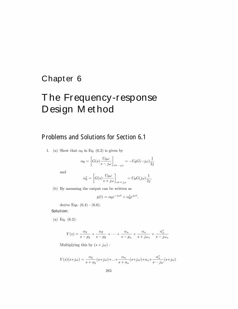
1. (a) Show that α0 in Eq. (6.2) is given by
α0 =
·G(s)
U0ω
s− jω¸s=−jω
= −U0G(−jω) 12j
and
α∗0 =·G(s)
U0ω
s+ jω
¸s=+jω
= U0G(jω)1
2j.
(b) By assuming the output can be written as
y(t) = α0e−jωt + α∗0e
jωt,
derive Eqs. (6.4) - (6.6).
Solution:
(a) Eq. (6.2):
Y (s) =α1
s− p1+
α2
s− p2+ · · ·+ αn
s− pn +αo
s+ jωo+
α∗os− jωo
Multiplying this by (s+ jω) :
Y (s)(s+jω) =α1
s+ a1(s+jω)+...+
αns+ an
(s+jω)+αo+α∗o
s− jω (s+jω)
283
284 CHAPTER 6. THE FREQUENCY-RESPONSE DESIGN METHOD
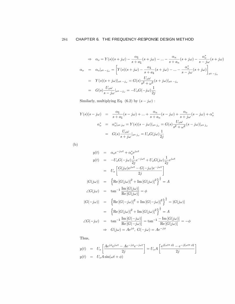
⇒ αo = Y (s)(s+ jω)− α1
s+ a1(s+ jω)− ...− αn
s+ an(s+ jω)− α∗o
s− jω (s+ jω)
αo = αo|s=−jω =·Y (s)(s+ jω)− α1
s+ a1(s+ jω)− ...− α∗o
s− jω (s+ jω)¸s=−jω
= Y (s)(s+ jω)|s=−jω = G(s)Uoω
s2 + ω2(s+ jω)|s=−jω
= G(s)Uoω
s− jω |s=−jω = −UoG(−jω)1
2j
Similarly, multiplying Eq. (6.2) by (s− jω) :
Y (s)(s− jω) =α1
s+ a1(s− jω) + ...+ αn
s+ an(s− jω) + αo
s+ jω(s− jω) + α∗o
α∗o = α∗o|s=jω = Y (s)(s− jω)|s=jω = G(s)Uoω
s2 + ω2(s− jω)|s=jω
= G(s)Uoω
s+ jω|s=jω = UoG(jω)
1
2j
(b)
y(t) = αoe−jωt + α∗oe
jωt
y(t) = −UoG(−jω) 12je−jωt + UoG(jω)
1
2jejωt
= Uo
·G(jω)ejωt −G(−jω)e−jωt
2j
¸|G(jω)| =
nRe [G(jω)]
2+ Im [G(jω)]
2o 1
2
= A
∠G(jω) = tan−1 Im [G(jω)]
Re [G(jω)]= φ
|G(−jω)| =nRe [G(−jω)]2 + Im [G(−jω)]2
o 12
= |G(jω)|
=nRe [G(jω)]2 + Im [G(jω)]2
o 12
= A
∠G(−jω) = tan−1 Im [G(−jω)]Re [G(−jω)] = tan
−1 − Im [G(jω)]Re [G(jω)]
= −φ
⇒ G(jω) = Aejφ, G(−jω) = Ae−jφ
Thus,
y(t) = Uo
·Aejφejωt −Ae−jφe−jωt
2j
¸= UoA
·ej(ωt+φ) − e−j(ωt+φ)
2j
¸y(t) = UoA sin(ωt+ φ)
285
where
A = |G(jω)| , φ = tan−1 Im [G(jω)]
Re [G(jω)]= ∠G(jω)
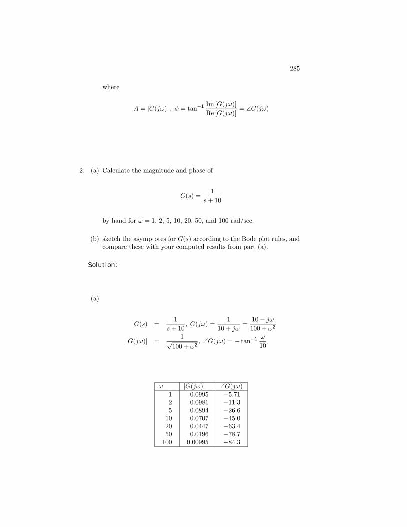
2. (a) Calculate the magnitude and phase of
G(s) =1
s+ 10
by hand for ω = 1, 2, 5, 10, 20, 50, and 100 rad/sec.
(b) sketch the asymptotes for G(s) according to the Bode plot rules, andcompare these with your computed results from part (a).
Solution:
(a)
G(s) =1
s+ 10, G(jω) =
1
10 + jω=10− jω100 + ω2
|G(jω)| =1√
100 + ω2, ∠G(jω) = − tan−1 ω
10
ω |G(jω)| ∠G(jω)125102050100
0.09950.09810.08940.07070.04470.01960.00995
−5.71−11.3−26.6−45.0−63.4−78.7−84.3
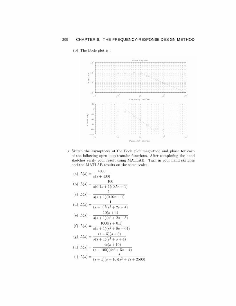
286 CHAPTER 6. THE FREQUENCY-RESPONSE DESIGN METHOD
(b) The Bode plot is :
10-1
100
101
102
103
10-3
10-2
10-1
100
Frequency (rad/sec)
Magnitude
B ode D iagram s
10-1
100
101
102
103
-100
-80
-60
-40
-20
0
20
Frequency (rad/sec)
Phase (deg)
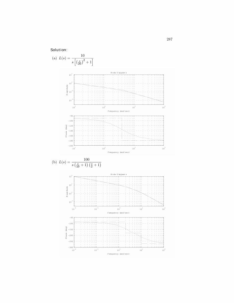
3. Sketch the asymptotes of the Bode plot magnitude and phase for eachof the following open-loop transfer functions. After completing the handsketches verify your result using MATLAB. Turn in your hand sketchesand the MATLAB results on the same scales.
(a) L(s) =4000
s(s+ 400)
(b) L(s) =100
s(0.1s+ 1)(0.5s+ 1)
(c) L(s) =1
s(s+ 1)(0.02s+ 1)
(d) L(s) =1
(s+ 1)2(s2 + 2s+ 4)
(e) L(s) =10(s+ 4)
s(s+ 1)(s2 + 2s+ 5)
(f) L(s) =1000(s+ 0.1)
s(s+ 1)(s2 + 8s+ 64)
(g) L(s) =(s+ 5)(s+ 3)
s(s+ 1)(s2 + s+ 4)
(h) L(s) =4s(s+ 10)
(s+ 100)(4s2 + 5s+ 4)
(i) L(s) =s
(s+ 1)(s+ 10)(s2 + 2s+ 2500)
287
Solution:
(a) L(s) =10
sh¡
s20
¢2+ 1i
101
102
103
104
10-4
10-2
100
102
Frequency (rad/sec)
Magnitude
B ode D iagram s
101
102
103
104
-200
-180
-160
-140
-120
-100
-80
Frequency (rad/sec)
Phase (deg)
(b) L(s) =100
s¡s
10 + 1¢ ¡
s2 + 1
¢
10-2
10-1
100
101
102
10-2
100
102
104
Frequency (rad/sec)
Magnitude
B ode D iagram s
10-2
10-1
100
101
102
-300
-250
-200
-150
-100
-50
Frequency (rad/sec)
Phase (deg)
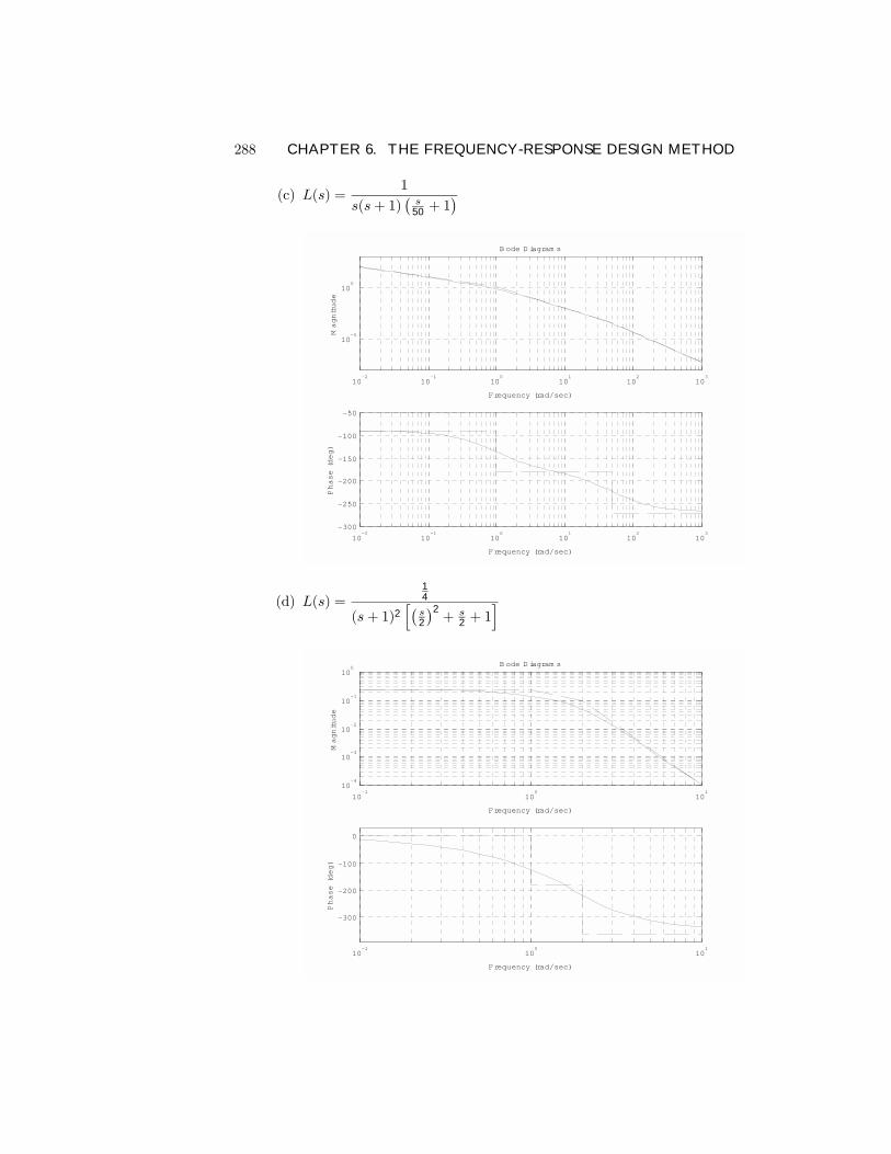
288 CHAPTER 6. THE FREQUENCY-RESPONSE DESIGN METHOD
(c) L(s) =1
s(s+ 1)¡s
50 + 1¢
10-2
10-1
100
101
102
103
10-5
100
Frequency (rad/sec)
Magnitude
B ode D iagram s
10-2
10-1
100
101
102
103
-300
-250
-200
-150
-100
-50
Frequency (rad/sec)
Phase (deg)
(d) L(s) =14
(s+ 1)2h¡
s2
¢2+ s
2 + 1i
10-1
100
101
10-4
10-3
10-2
10-1
100
Frequency (rad/sec)
Magnitude
B ode D iagram s
10-1
100
101
-300
-200
-100
0
Frequency (rad/sec)
Phase (deg)
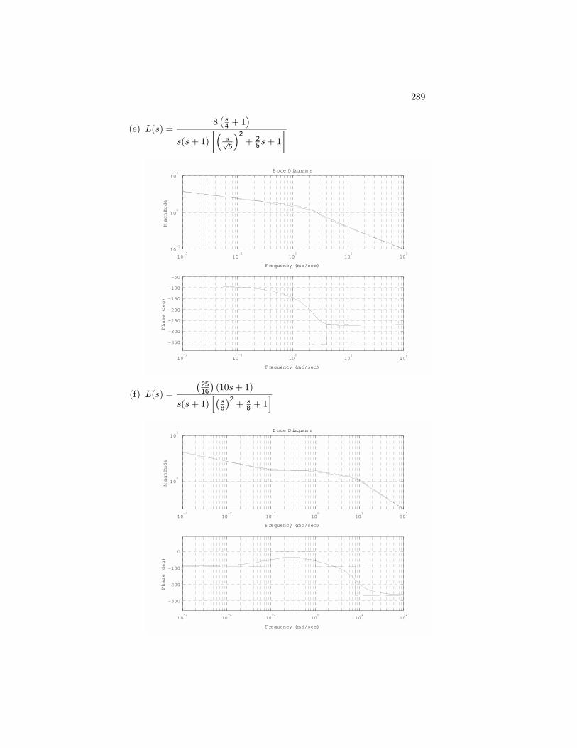
289
(e) L(s) =8¡s4 + 1
¢s(s+ 1)
·³s√5
´2
+ 25s+ 1
¸
10-2
10-1
100
101
102
10-5
100
105
Frequency (rad/sec)
Magnitude
B ode D iagram s
10-2
10-1
100
101
102
-350
-300
-250
-200
-150
-100
-50
Frequency (rad/sec)
Phase (deg)
(f) L(s) =
¡2516
¢(10s+ 1)
s(s+ 1)h¡
s8
¢2+ s
8 + 1i
10-3
10-2
10-1
100
101
102
100
105
Frequency (rad/sec)
Magnitude
B ode D iagram s
10-3
10-2
10-1
100
101
102
-300
-200
-100
0
Frequency (rad/sec)
Phase (deg)
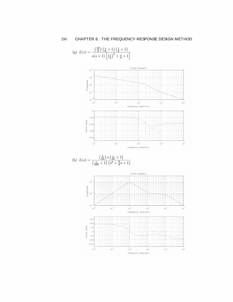
290 CHAPTER 6. THE FREQUENCY-RESPONSE DESIGN METHOD
(g) L(s) =
¡154
¢ ¡s5 + 1
¢ ¡s3 + 1
¢s(s+ 1)
h¡s2
¢2+ s
4 + 1i
10-2
10-1
100
101
102
10-4
10-2
100
102
104
Frequency (rad/sec)
Magnitude
B ode D iagram s
10-2
10-1
100
101
102
-400
-300
-200
-100
0
Frequency (rad/sec)
Phase (deg)
(h) L(s) =
¡1
10
¢s¡s
10 + 1¢¡
s100 + 1
¢ ¡s2 + 5
4s+ 1¢
10-2
10-1
100
101
102
103
10-3
10-2
10-1
Frequency (rad/sec)
Magnitude
B ode D iagram s
10-2
10-1
100
101
102
103
-150
-100
-50
0
50
100
150
Frequency (rad/sec)
Phase (deg)
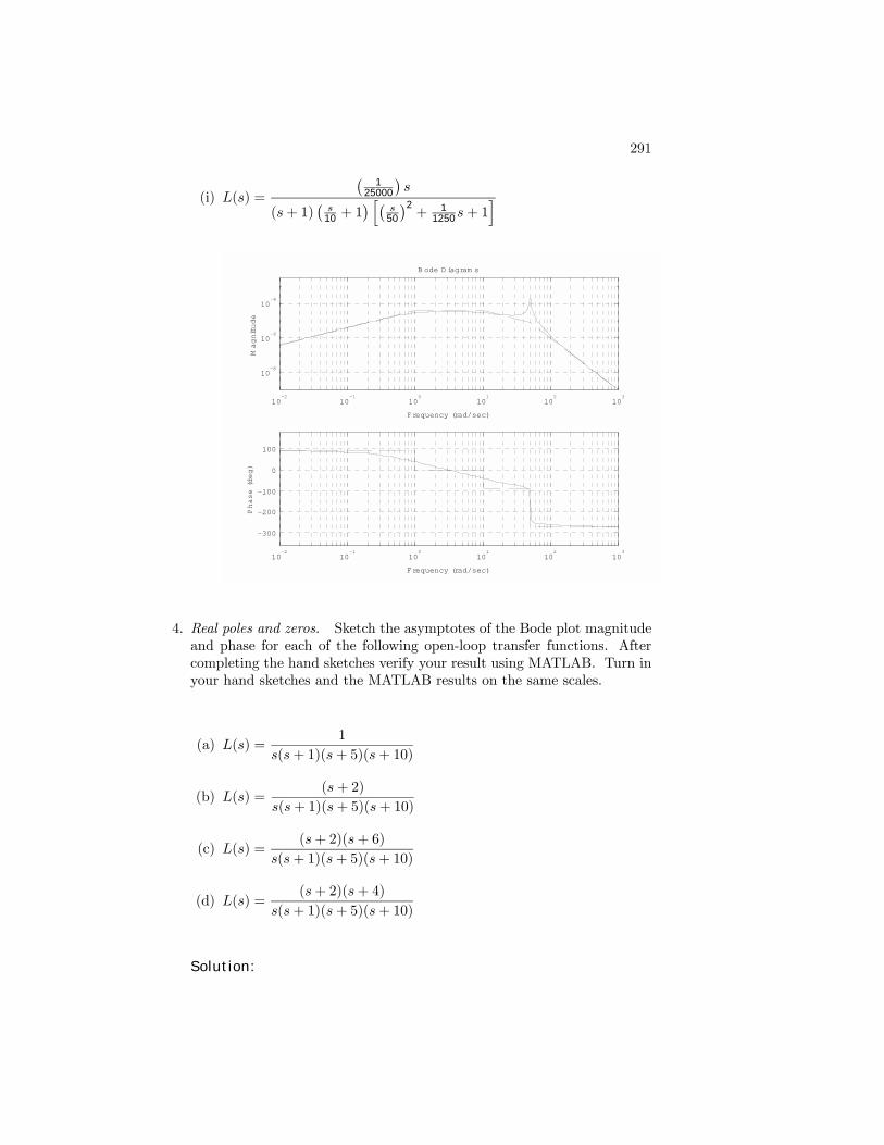
291
(i) L(s) =
¡1
25000
¢s
(s+ 1)¡s
10 + 1¢ h¡
s50
¢2+ 1
1250s+ 1i
10-2
10-1
100
101
102
103
10-8
10-6
10-4
Frequency (rad/sec)
Magnitude
B ode D iagram s
10-2
10-1
100
101
102
103
-300
-200
-100
0
100
Frequency (rad/sec)
Phase (deg)
4. Real poles and zeros. Sketch the asymptotes of the Bode plot magnitudeand phase for each of the following open-loop transfer functions. Aftercompleting the hand sketches verify your result using MATLAB. Turn inyour hand sketches and the MATLAB results on the same scales.
(a) L(s) =1
s(s+ 1)(s+ 5)(s+ 10)
(b) L(s) =(s+ 2)
s(s+ 1)(s+ 5)(s+ 10)
(c) L(s) =(s+ 2)(s+ 6)
s(s+ 1)(s+ 5)(s+ 10)
(d) L(s) =(s+ 2)(s+ 4)
s(s+ 1)(s+ 5)(s+ 10)
Solution:
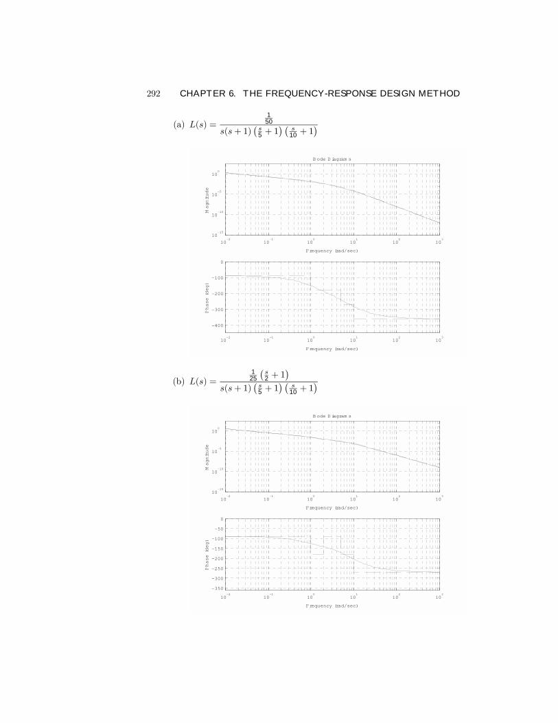
292 CHAPTER 6. THE FREQUENCY-RESPONSE DESIGN METHOD
(a) L(s) =1
50
s(s+ 1)¡s5 + 1
¢ ¡s
10 + 1¢
10-2
10-1
100
101
102
103
10-15
10-10
10-5
100
Frequency (rad/sec)
Magnitude
B ode D iagram s
10-2
10-1
100
101
102
103
-400
-300
-200
-100
0
Frequency (rad/sec)
Phase (deg)
(b) L(s) =1
25
¡s2 + 1
¢s(s+ 1)
¡s5 + 1
¢ ¡s
10 + 1¢
10-2
10-1
100
101
102
103
10-15
10-10
10-5
100
Frequency (rad/sec)
Magnitude
B ode D iagram s
10-2
10-1
100
101
102
103
-350
-300
-250
-200
-150
-100
-50
0
Frequency (rad/sec)
Phase (deg)
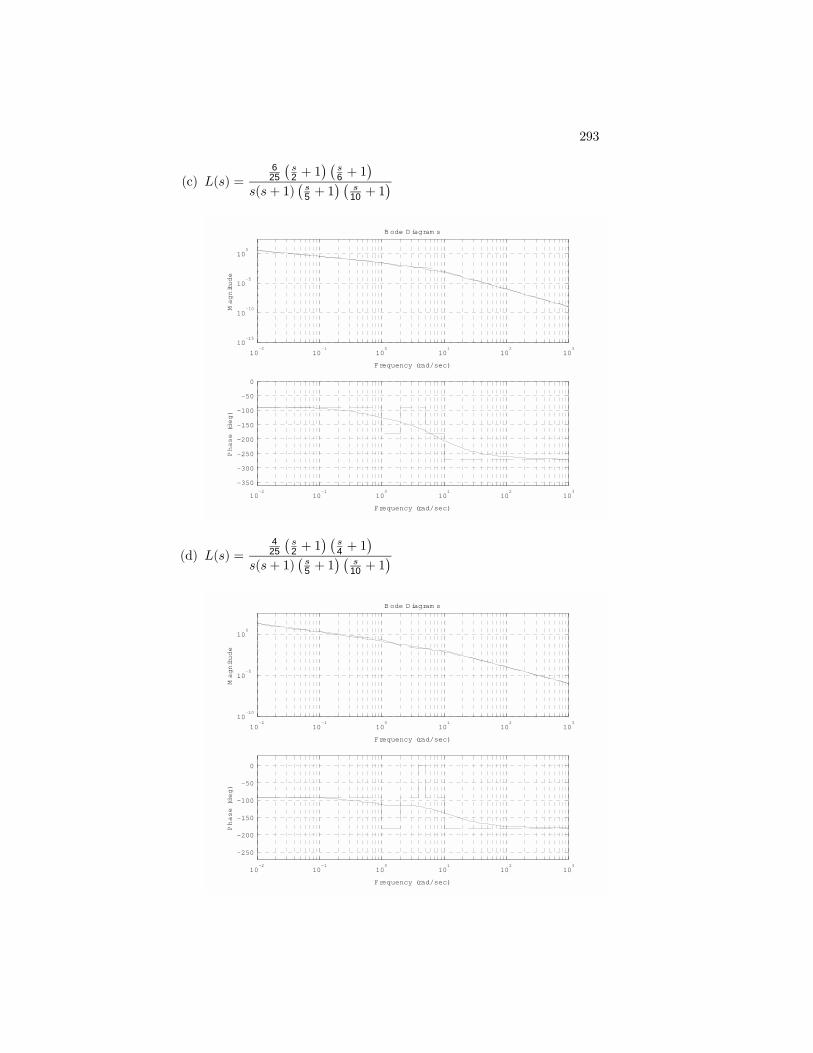
293
(c) L(s) =6
25
¡s2 + 1
¢ ¡s6 + 1
¢s(s+ 1)
¡s5 + 1
¢ ¡s
10 + 1¢
10-2
10-1
100
101
102
103
10-15
10-10
10-5
100
Frequency (rad/sec)
Magnitude
B ode D iagram s
10-2
10-1
100
101
102
103
-350
-300
-250
-200
-150
-100
-50
0
Frequency (rad/sec)
Phase (deg)
(d) L(s) =4
25
¡s2 + 1
¢ ¡s4 + 1
¢s(s+ 1)
¡s5 + 1
¢ ¡s
10 + 1¢
10-2
10-1
100
101
102
103
10-10
10-5
100
Frequency (rad/sec)
Magnitude
B ode D iagram s
10-2
10-1
100
101
102
103
-250
-200
-150
-100
-50
0
Frequency (rad/sec)
Phase (deg)
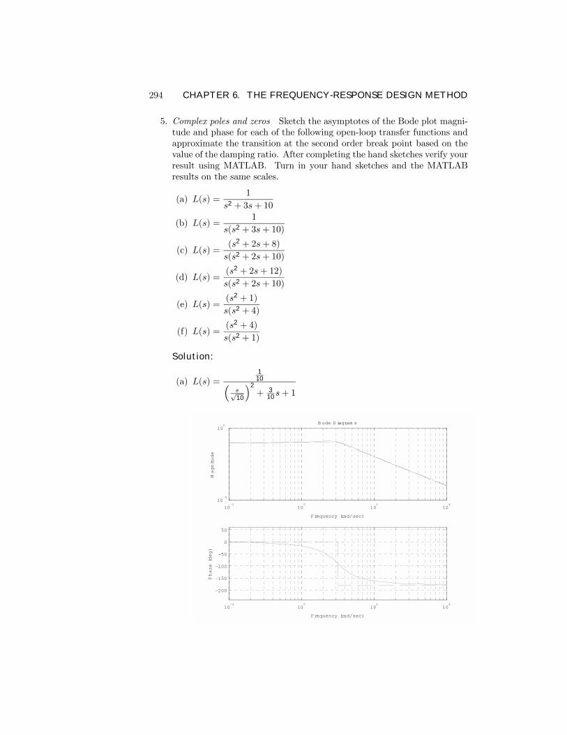
294 CHAPTER 6. THE FREQUENCY-RESPONSE DESIGN METHOD
5. Complex poles and zeros Sketch the asymptotes of the Bode plot magni-tude and phase for each of the following open-loop transfer functions andapproximate the transition at the second order break point based on thevalue of the damping ratio. After completing the hand sketches verify yourresult using MATLAB. Turn in your hand sketches and the MATLABresults on the same scales.
(a) L(s) =1
s2 + 3s+ 10
(b) L(s) =1
s(s2 + 3s+ 10)
(c) L(s) =(s2 + 2s+ 8)
s(s2 + 2s+ 10)
(d) L(s) =(s2 + 2s+ 12)
s(s2 + 2s+ 10)
(e) L(s) =(s2 + 1)
s(s2 + 4)
(f) L(s) =(s2 + 4)
s(s2 + 1)
Solution:
(a) L(s) =1
10³s√10
´2
+ 310s+ 1
10-1
100
101
102
10-5
100
Frequency (rad/sec)
Magnitude
B ode D iagram s
10-1
100
101
102
-200
-150
-100
-50
0
50
Frequency (rad/sec)
Phase (deg)
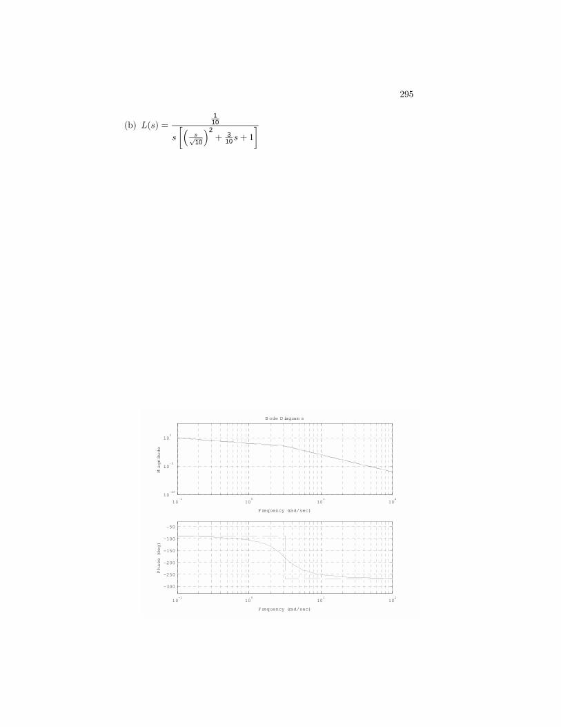
295
(b) L(s) =1
10
s
·³s√10
´2
+ 310s+ 1
¸
10-1
100
101
102
10-10
10-5
100
Frequency (rad/sec)
Magnitude
B ode D iagram s
10-1
100
101
102
-300
-250
-200
-150
-100
-50
Frequency (rad/sec)
Phase (deg)
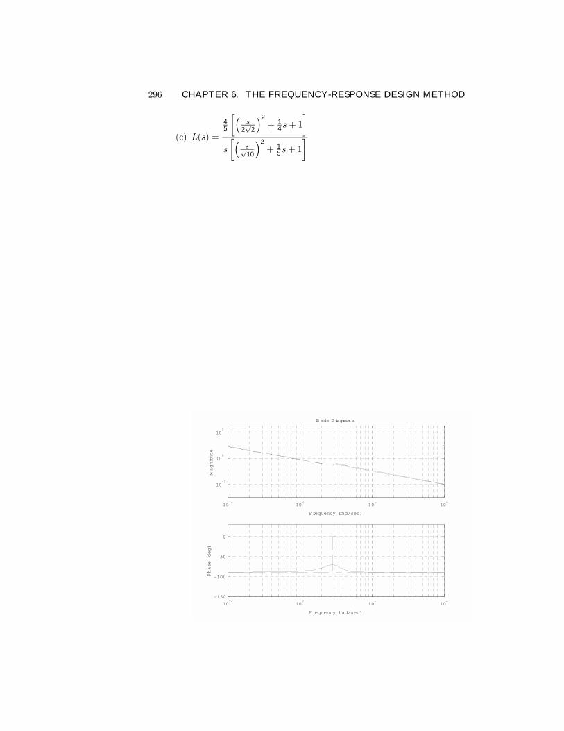
296 CHAPTER 6. THE FREQUENCY-RESPONSE DESIGN METHOD
(c) L(s) =
45
·³s
2√
2
´2
+ 14s+ 1
¸s
·³s√10
´2
+ 15s+ 1
¸
10-1
100
101
102
10-2
100
102
Frequency (rad/sec)
Magnitude
B ode D iagram s
10-1
100
101
102
-150
-100
-50
0
Frequency (rad/sec)
Phase (deg)
297
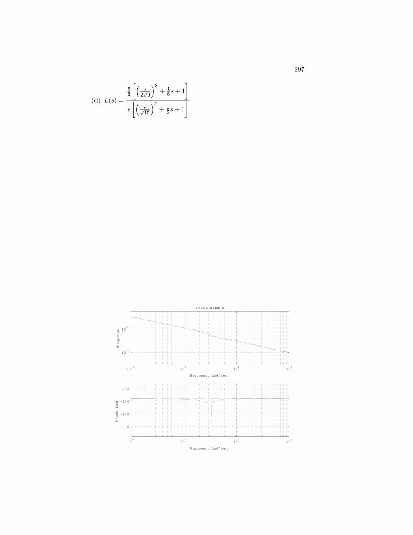
(d) L(s) =
65
·³s
2√
3
´2
+ 16s+ 1
¸s
·³s√10
´2
+ 15s+ 1
¸
10-1
100
101
102
10-2
100
Frequency (rad/sec)
Magnitude
B ode D iagram s
10-1
100
101
102
-200
-150
-100
-50
Frequency (rad/sec)
Phase (deg)
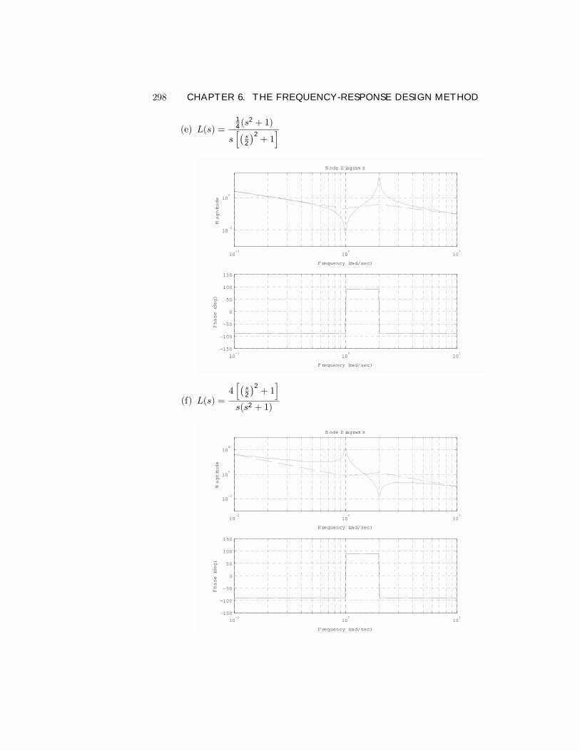
298 CHAPTER 6. THE FREQUENCY-RESPONSE DESIGN METHOD
(e) L(s) =14(s
2 + 1)
sh¡
s2
¢2+ 1i
10-1
100
101
10-2
100
Frequency (rad/sec)
Magnitude
B ode D iagram s
10-1
100
101
-150
-100
-50
0
50
100
150
Frequency (rad/sec)
Phase (deg)
(f) L(s) =4h¡
s2
¢2+ 1i
s(s2 + 1)
10-1
100
101
10-2
100
102
Frequency (rad/sec)
Magnitude
B ode D iagram s
10-1
100
101
-150
-100
-50
0
50
100
150
Frequency (rad/sec)
Phase (deg)
299
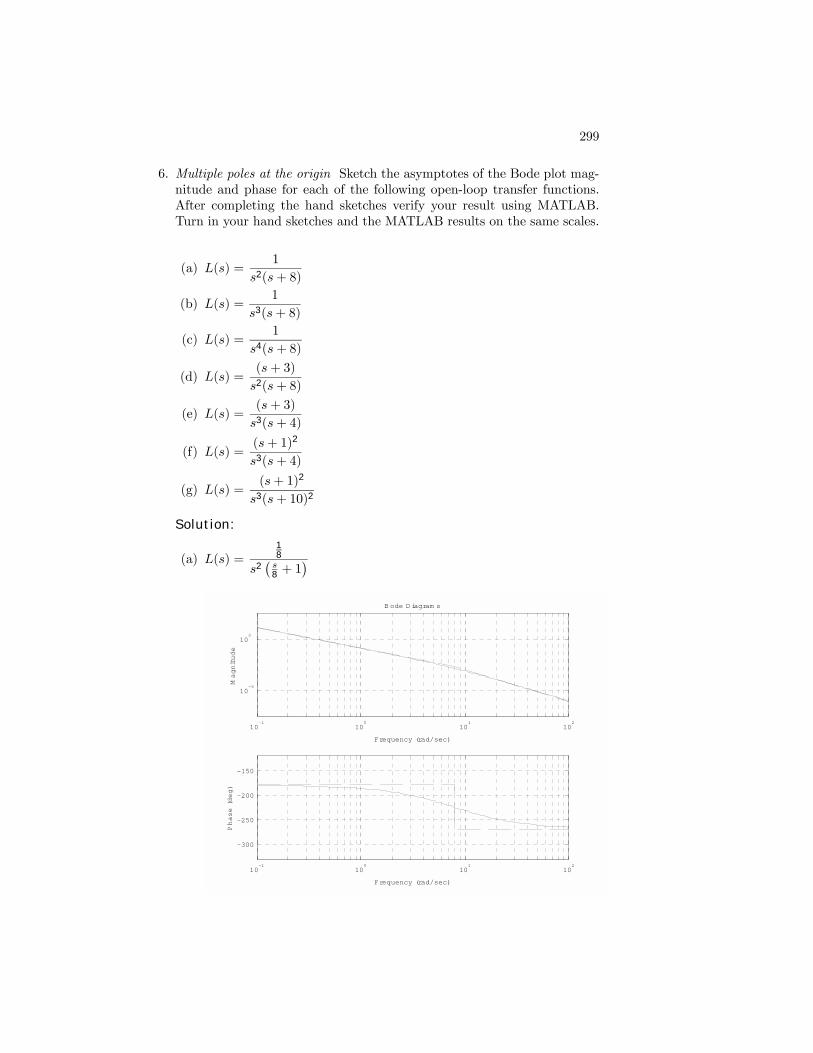
6. Multiple poles at the origin Sketch the asymptotes of the Bode plot mag-nitude and phase for each of the following open-loop transfer functions.After completing the hand sketches verify your result using MATLAB.Turn in your hand sketches and the MATLAB results on the same scales.
(a) L(s) =1
s2(s+ 8)
(b) L(s) =1
s3(s+ 8)
(c) L(s) =1
s4(s+ 8)
(d) L(s) =(s+ 3)
s2(s+ 8)
(e) L(s) =(s+ 3)
s3(s+ 4)
(f) L(s) =(s+ 1)2
s3(s+ 4)
(g) L(s) =(s+ 1)2
s3(s+ 10)2
Solution:
(a) L(s) =18
s2¡s8 + 1
¢
10-1
100
101
102
10-5
100
Frequency (rad/sec)
Magnitude
B ode D iagram s
10-1
100
101
102
-300
-250
-200
-150
Frequency (rad/sec)
Phase (deg)
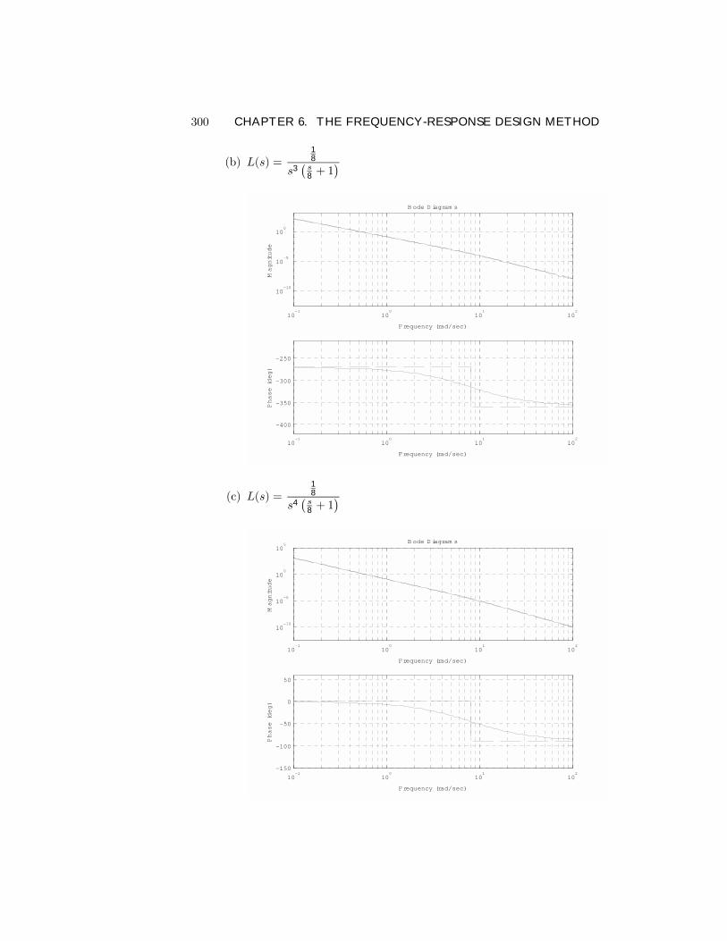
300 CHAPTER 6. THE FREQUENCY-RESPONSE DESIGN METHOD
(b) L(s) =18
s3¡s8 + 1
¢
10-1
100
101
102
10-10
10-5
100
Frequency (rad/sec)
Magnitude
B ode D iagram s
10-1
100
101
102
-400
-350
-300
-250
Frequency (rad/sec)
Phase (deg)
(c) L(s) =18
s4¡s8 + 1
¢
10-1
100
101
102
10-10
10-5
100
105
Frequency (rad/sec)
Magnitude
B ode D iagram s
10-1
100
101
102
-150
-100
-50
0
50
Frequency (rad/sec)
Phase (deg)
301
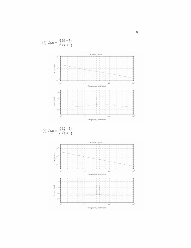
(d) L(s) =38
¡s3 + 1
¢s2¡s8 + 1
¢
10-1
100
101
102
10-5
100
105
Frequency (rad/sec)
Magnitude
B ode D iagram s
10-1
100
101
102
-200
-150
-100
-50
Frequency (rad/sec)
Phase (deg)
(e) L(s) =34
¡s3 + 1
¢s3¡s4 + 1
¢
10-1
100
101
102
10-5
100
105
Frequency (rad/sec)
Magnitude
B ode D iagram s
10-1
100
101
102
-300
-250
-200
-150
Frequency (rad/sec)
Phase (deg)
302 CHAPTER 6. THE FREQUENCY-RESPONSE DESIGN METHOD
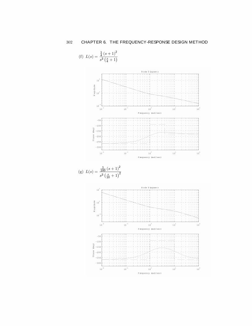
(f) L(s) =14 (s+ 1)
2
s3¡s4 + 1
¢
10-2
10-1
100
101
102
10-5
100
105
Frequency (rad/sec)
Magnitude
B ode D iagram s
10-2
10-1
100
101
102
-300
-250
-200
-150
-100
-50
Frequency (rad/sec)
Phase (deg)
(g) L(s) =1
100 (s+ 1)2
s3¡s
10 + 1¢2
10-2
10-1
100
101
102
10-5
100
105
Frequency (rad/sec)
Magnitude
B ode D iagram s
10-2
10-1
100
101
102
-300
-250
-200
-150
-100
-50
Frequency (rad/sec)
Phase (deg)
303
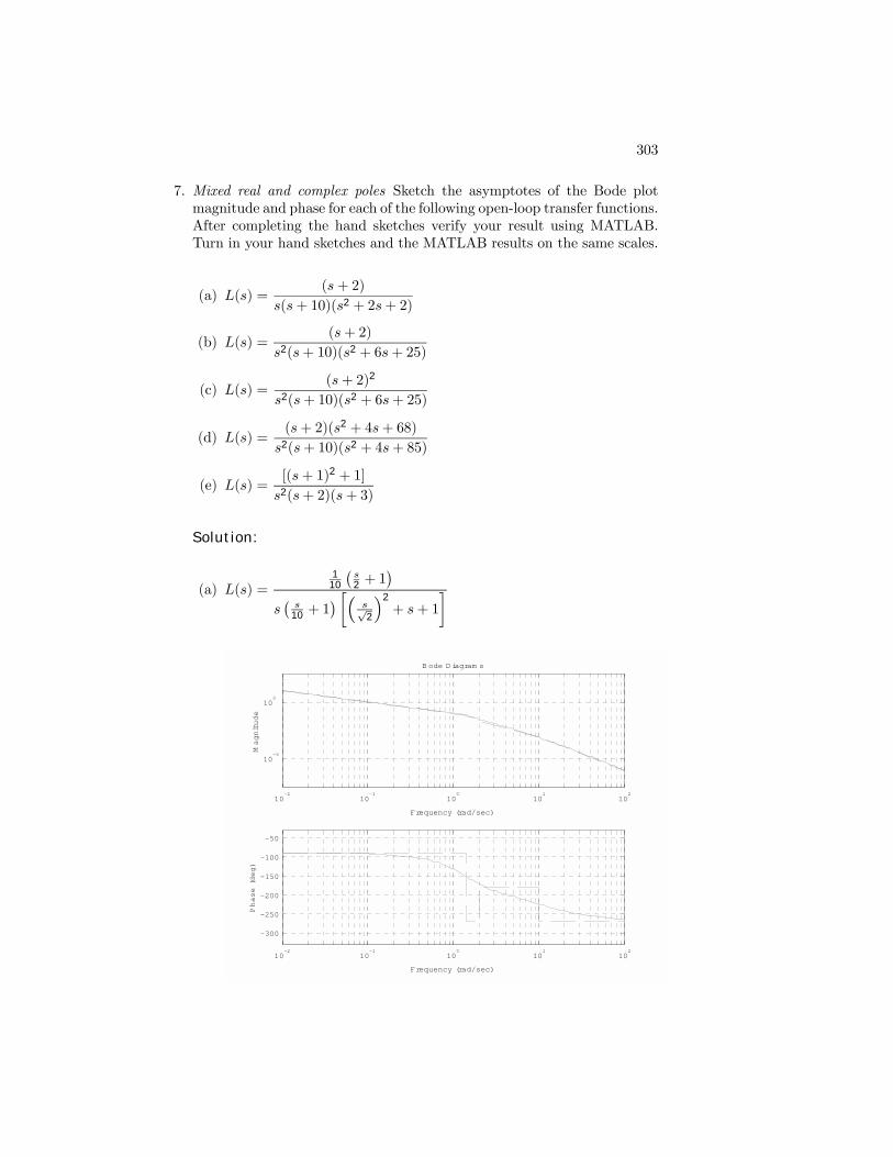
7. Mixed real and complex poles Sketch the asymptotes of the Bode plotmagnitude and phase for each of the following open-loop transfer functions.After completing the hand sketches verify your result using MATLAB.Turn in your hand sketches and the MATLAB results on the same scales.
(a) L(s) =(s+ 2)
s(s+ 10)(s2 + 2s+ 2)
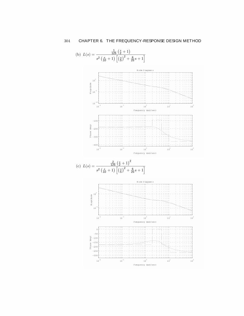
(b) L(s) =(s+ 2)
s2(s+ 10)(s2 + 6s+ 25)
(c) L(s) =(s+ 2)2
s2(s+ 10)(s2 + 6s+ 25)
(d) L(s) =(s+ 2)(s2 + 4s+ 68)
s2(s+ 10)(s2 + 4s+ 85)
(e) L(s) =[(s+ 1)2 + 1]
s2(s+ 2)(s+ 3)
Solution:
(a) L(s) =1
10
¡s2 + 1
¢s¡s
10 + 1¢ ·³
s√2
´2
+ s+ 1
¸
10-2
10-1
100
101
102
10-5
100
Frequency (rad/sec)
Magnitude
B ode D iagram s
10-2
10-1
100
101
102
-300
-250
-200
-150
-100
-50
Frequency (rad/sec)
Phase (deg)
304 CHAPTER 6. THE FREQUENCY-RESPONSE DESIGN METHOD
(b) L(s) =1
125
¡s2 + 1
¢s2¡s
10 + 1¢ h¡
s5
¢2+ 6
25s+ 1i
10-2
10-1
100
101
102
10-10
10-5
100
Frequency (rad/sec)
Magnitude
B ode D iagram s
10-2
10-1
100
101
102
-400
-300
-200
-100
Frequency (rad/sec)
Phase (deg)
(c) L(s) =2
125
¡s2 + 1
¢2
s2¡s
10 + 1¢ h¡
s5
¢2+ 6
25s+ 1i
10-2
10-1
100
101
102
10-5
100
Frequency (rad/sec)
Magnitude
B ode D iagram s
10-2
10-1
100
101
102
-300
-250
-200
-150
-100
-50
0
Frequency (rad/sec)
Phase (deg)
305
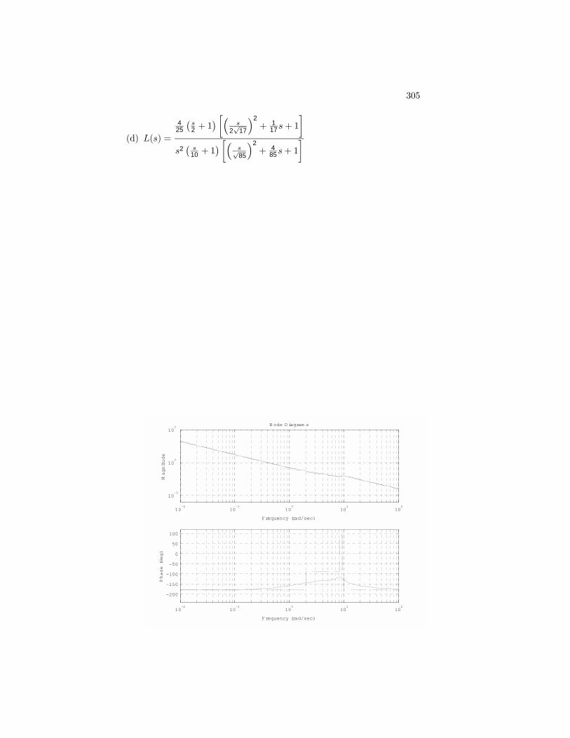
(d) L(s) =
425
¡s2 + 1
¢ ·³s
2√
17
´2
+ 117s+ 1
¸s2¡s
10 + 1¢ ·³
s√85
´2
+ 485s+ 1
¸
10-2
10-1
100
101
102
10-5
100
105
Frequency (rad/sec)
Magnitude
B ode D iagram s
10-2
10-1
100
101
102
-200
-150
-100
-50
0
50
100
Frequency (rad/sec)
Phase (deg)
306 CHAPTER 6. THE FREQUENCY-RESPONSE DESIGN METHOD
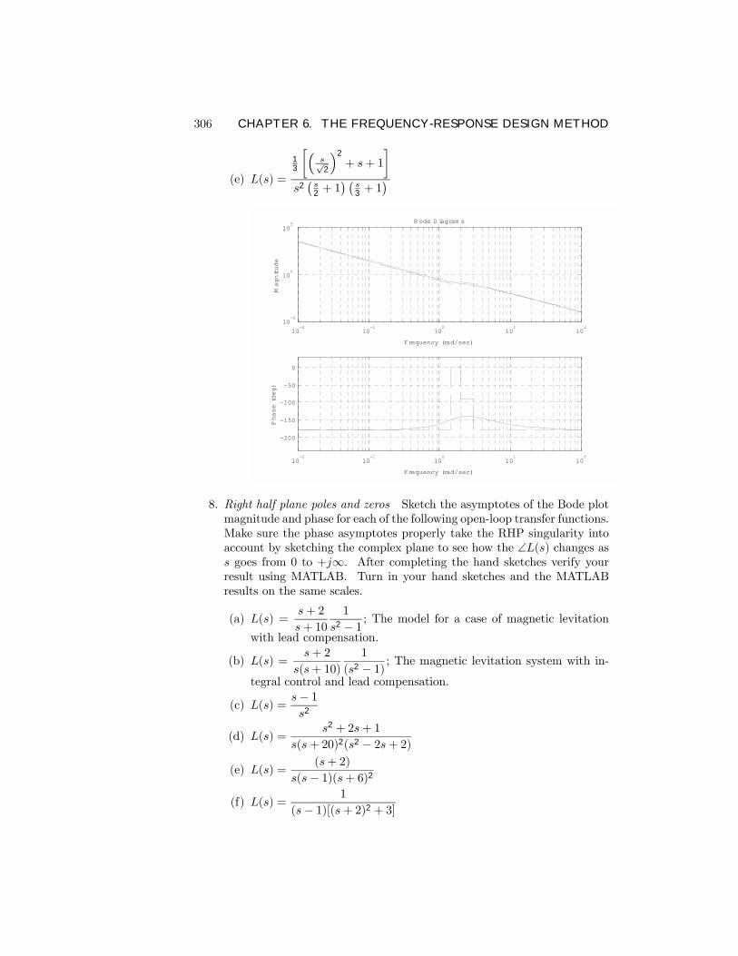
(e) L(s) =
13
·³s√2
´2
+ s+ 1
¸s2¡s2 + 1
¢ ¡s3 + 1
¢
10-2
10-1
100
101
102
10-5
100
105
Frequency (rad/sec)
Magnitude
B ode D iagram s
10-2
10-1
100
101
102
-200
-150
-100
-50
0
Frequency (rad/sec)
Phase (deg)
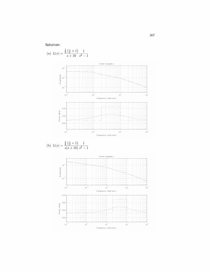
8. Right half plane poles and zeros Sketch the asymptotes of the Bode plotmagnitude and phase for each of the following open-loop transfer functions.Make sure the phase asymptotes properly take the RHP singularity intoaccount by sketching the complex plane to see how the ∠L(s) changes ass goes from 0 to +j∞. After completing the hand sketches verify yourresult using MATLAB. Turn in your hand sketches and the MATLABresults on the same scales.
(a) L(s) =s+ 2
s+ 10
1
s2 − 1 ; The model for a case of magnetic levitationwith lead compensation.
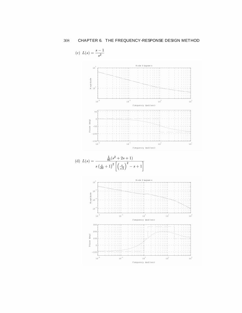
(b) L(s) =s+ 2
s(s+ 10)
1
(s2 − 1) ; The magnetic levitation system with in-
tegral control and lead compensation.
(c) L(s) =s− 1s2
(d) L(s) =s2 + 2s+ 1
s(s+ 20)2(s2 − 2s+ 2)(e) L(s) =
(s+ 2)
s(s− 1)(s+ 6)2
(f) L(s) =1
(s− 1)[(s+ 2)2 + 3]
307
Solution:
(a) L(s) =15
¡s2 + 1
¢s+ 10
1
s2 − 1
10-1
100
101
102
10-4
10-2
100
Frequency (rad/sec)
Magnitude
B ode D iagram s
10-1
100
101
102
-200
-150
-100
Frequency (rad/sec)
Phase (deg)
(b) L(s) =15
¡s2 + 1
¢s(s+ 10)
1
s2 − 1
10-2
10-1
100
101
102
10-5
100
Frequency (rad/sec)
Magnitude
B ode D iagram s
10-2
10-1
100
101
102
-300
-250
-200
-150
Frequency (rad/sec)
Phase (deg)
308 CHAPTER 6. THE FREQUENCY-RESPONSE DESIGN METHOD
(c) L(s) =s− 1s2
10-2
10-1
100
101
100
105
Frequency (rad/sec)
Magnitude
B ode D iagram s
10-2
10-1
100
101
-150
-100
-50
0
50
Frequency (rad/sec)
Phase (deg)
(d) L(s) =1
40(s2 + 2s+ 1)
s¡s
20 + 1¢2·³
s√2
´2
− s+ 1¸
10-2
10-1
100
101
102
10-6
10-4
10-2
100
Frequency (rad/sec)
Magnitude
B ode D iagram s
10-2
10-1
100
101
102
-100
0
100
200
300
Frequency (rad/sec)
Phase (deg)
309
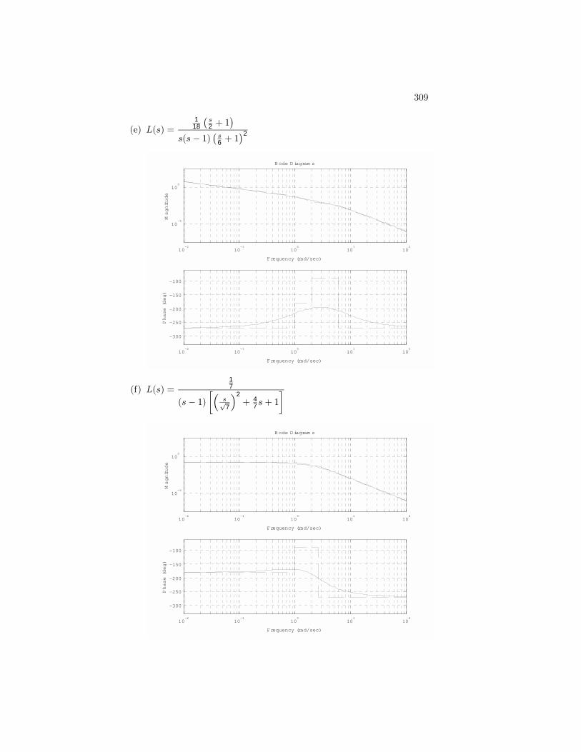
(e) L(s) =1
18
¡s2 + 1
¢s(s− 1) ¡ s6 + 1¢2
10-2
10-1
100
101
102
10-5
100
Frequency (rad/sec)
Magnitude
B ode D iagram s
10-2
10-1
100
101
102
-300
-250
-200
-150
-100
Frequency (rad/sec)
Phase (deg)
(f) L(s) =17
(s− 1)·³
s√7
´2
+ 47s+ 1
¸
10-2
10-1
100
101
102
10-5
100
Frequency (rad/sec)
Magnitude
B ode D iagram s
10-2
10-1
100
101
102
-300
-250
-200
-150
-100
Frequency (rad/sec)
Phase (deg)
310 CHAPTER 6. THE FREQUENCY-RESPONSE DESIGN METHOD
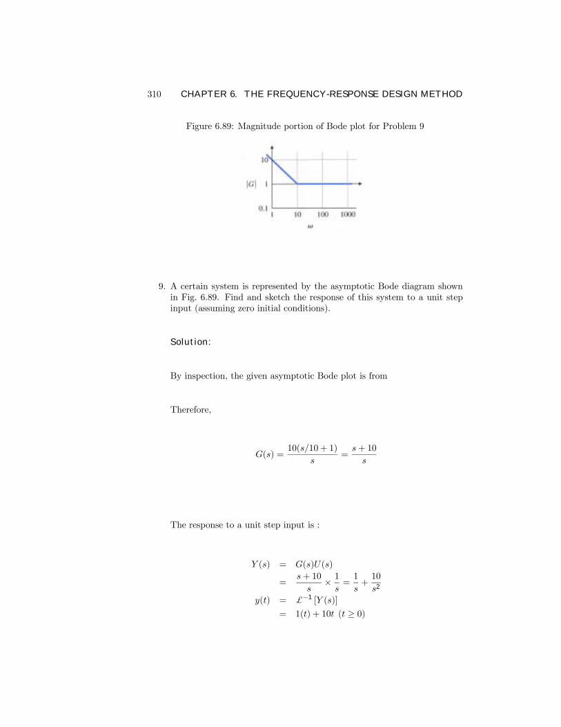
Figure 6.89: Magnitude portion of Bode plot for Problem 9
9. A certain system is represented by the asymptotic Bode diagram shownin Fig. 6.89. Find and sketch the response of this system to a unit stepinput (assuming zero initial conditions).
Solution:
By inspection, the given asymptotic Bode plot is from
Therefore,
G(s) =10(s/10 + 1)
s=s+ 10
s
The response to a unit step input is :
Y (s) = G(s)U(s)
=s+ 10
s× 1s=1
s+10
s2
y(t) = £−1 [Y (s)]
= 1(t) + 10t (t ≥ 0)

311
0 0.5 1 1.5 20
5
10
15
20
25
Time (sec)
y(t)
Unit Step Response
10. Prove that a magnitude slope of −1 in a Bode plot corresponds to −20 dbper decade or -6 db per octave.
Solution:
The deÞnition of db is db = 20 log |G| (1)
Assume slope = d(log|G|)d(logω) = −1 (2)
(2) =⇒ log |G| = − logω + c (c is a constant.) (3)
(1) and (3) =⇒ db = −20 logω + 20cDifferentiating this,
d (db)
d (logω)= −20
Thus, a magnitude slope of -1 corresponds to -20 db per decade.
Similarly,d (db)
d (log2 ω)=
d (db)
d³
logωlog 2
´ + −6Thus, a magnitude slope of -1 corresponds to -6 db per octave.
11. A normalized second-order system with a damping ratio ζ = 0.5 and anadditional zero is given by
G(s) =s/a+ 1
s2 + s+ 1.
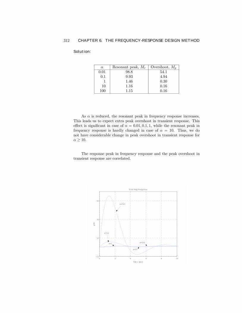
Use MATLAB to compare the Mp from the step response of the systemfor a = 0.01, 0.1, 1, 10, and 100 with the Mr from the frequency responseof each case. Is there a correlation between Mr and Mp?
312 CHAPTER 6. THE FREQUENCY-RESPONSE DESIGN METHOD
Solution:
α Resonant peak, Mr Overshoot, Mp
0.010.1110100
98.89.931.461.161.15
54.14.940.300.160.16
As α is reduced, the resonant peak in frequency response increases.This leads us to expect extra peak overshoot in transient response. Thiseffect is signiÞcant in case of α = 0.01, 0.1, 1, while the resonant peak infrequency response is hardly changed in case of α = 10. Thus, we donot have considerable change in peak overshoot in transient response forα ≥ 10.
The response peak in frequency response and the peak overshoot intransient response are correlated.
0 2 4 6 8 10-10
10
30
50
Tim e (sec)
y(t)
U nit Step Response
a=0.01
a=0.1
a=1
a=10
a=100
313
10-2
10-1
100
101
102
10-5
100
Frequency (rad/sec)
Magnitude
B ode D iagram s
a=0.01
a=0.1
a=1a=10
a=100
10-2
10-1
100
101
102
-200
-100
0
100
Frequency (rad/sec)
Phase (deg)
a=0.01
a=0.1 a=1
a=10a=100
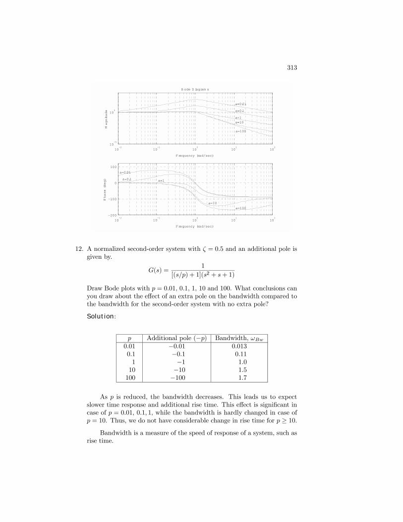
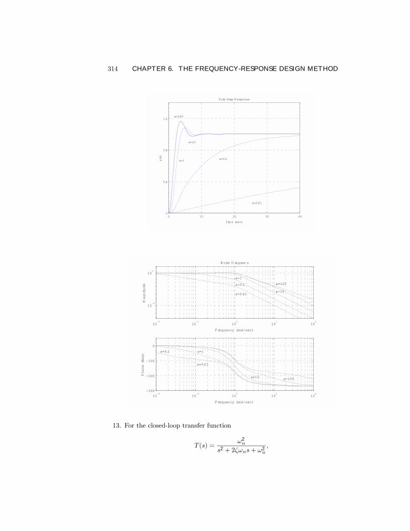
12. A normalized second-order system with ζ = 0.5 and an additional pole isgiven by.
G(s) =1
[(s/p) + 1](s2 + s+ 1)
Draw Bode plots with p = 0.01, 0.1, 1, 10 and 100. What conclusions canyou draw about the effect of an extra pole on the bandwidth compared tothe bandwidth for the second-order system with no extra pole?
Solution:
p Additional pole (−p) Bandwidth, ωBw0.010.1110100
−0.01−0.1−1−10−100
0.0130.111.01.51.7
As p is reduced, the bandwidth decreases. This leads us to expectslower time response and additional rise time. This effect is signiÞcant incase of p = 0.01, 0.1, 1, while the bandwidth is hardly changed in case ofp = 10. Thus, we do not have considerable change in rise time for p ≥ 10.
Bandwidth is a measure of the speed of response of a system, such asrise time.
314 CHAPTER 6. THE FREQUENCY-RESPONSE DESIGN METHOD
0 10 20 30 400
0.4
0.8
1.2
Tim e (sec)
y(t)
U nit Step Response
a=0.01
a=0.1a=1
a=10
a=100
10-2
10-1
100
101
102
10-5
100
Frequency (rad/sec)
Magnitude
B ode D iagram s
a=0.01
a=0.1
a=1
a=10
a=100
10-2
10-1
100
101
102
-300
-200
-100
0
Frequency (rad/sec)
Phase (deg)
a=0.01
a=0.1 a=1
a=10 a=100
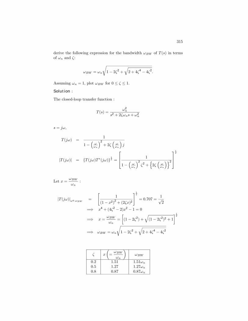
13. For the closed-loop transfer function
T (s) =ω2n
s2 + 2ζωns+ ω2n
,
315
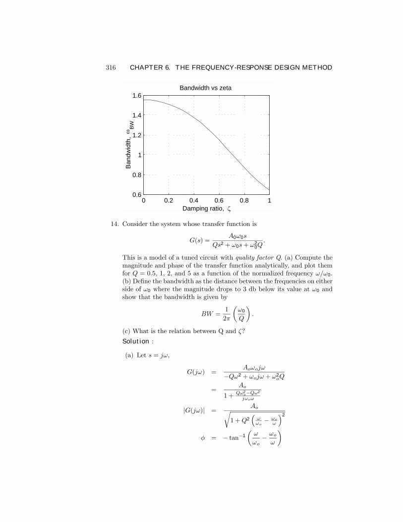
derive the following expression for the bandwidth ωBW of T (s) in termsof ωn and ζ:
ωBW = ωn
r1− 2ζ2 +
q2 + 4ζ4 − 4ζ2.
Assuming ωn = 1, plot ωBW for 0 ≤ ζ ≤ 1.Solution :
The closed-loop transfer function :
T (s) =ω2n
s2 + 2ζωns+ ω2n
s = jω,
T (jω) =1
1−³ωωn
´2
+ 2ζ³ωωn
´j
|T (jω)| = T (jω)T ∗(jω) 12 =
1
1−³ωωn
´2
ζ2 +n2ζ³ωωn
´o2
12
Let x =ωBWωn
:
|T (jω)|ω=ωBW=
"1
(1− x2)2 + (2ζx)2
# 12
= 0.707 =1√2
=⇒ x4 + (4ζ2 − 2)x2 − 1 = 0
=⇒ x =ωBWωn
=
·(1− 2ζ2) +
q(1− 2ζ2)2 + 1
¸ 12
=⇒ ωBW = ωn
r1− 2ζ2 +
q2 + 4ζ4 − 4ζ2
ζ x
µ=ωBWωn
¶ωBW
0.20.50.8
1.511.270.87
1.51ωn1.27ωn0.87ωn
316 CHAPTER 6. THE FREQUENCY-RESPONSE DESIGN METHOD
0 0.2 0.4 0.6 0.8 10.6
0.8
1
1.2
1.4
1.6
Damping ratio,
Band
wid
th,
BW
Bandwidth vs zeta
14. Consider the system whose transfer function is
G(s) =A0ω0s
Qs2 + ω0s+ ω20Q.
This is a model of a tuned circuit with quality factor Q. (a) Compute themagnitude and phase of the transfer function analytically, and plot themfor Q = 0.5, 1, 2, and 5 as a function of the normalized frequency ω/ω0.(b) DeÞne the bandwidth as the distance between the frequencies on eitherside of ω0 where the magnitude drops to 3 db below its value at ω0 andshow that the bandwidth is given by
BW =1
2π
µω0
Q
¶.
(c) What is the relation between Q and ζ?
Solution :
(a) Let s = jω,
G(jω) =Aoωojω
−Qω2 + ωojω + ω2oQ
=Ao
1 +Qω2
o−Qω2
jωoω
|G(jω)| =Aor
1 +Q2³ωωo− ωo
ω
´2
φ = − tan−1
µω
ωo− ωoω
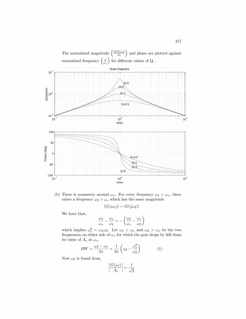
317
The normalized magnitude³QG(jω)Ao
´and phase are plotted against
normalized frequency³ωωo
´for different values of Q. .
10-1 100 10110-1
100
101
w/wo
QG
(jw)/A
o
Bode Diagrams
Q=0.5
Q=1
Q=2Q=5
10-1 100 101-100
-50
0
50
100
Phas
e (d
eg)
w/wo
Q=0.5
Q=1Q=2
Q=5
(b) There is symmetry around ωo. For every frequency ω1 < ωo, thereexists a frequency ω2 > ωo which has the same magnitude
|G(jω1)| = |G(jω2)|We have that,
ω1
ωo− ωoω1= −
µω2
ωo− ωoω2
¶which implies ω2
o = ω1ω2. Let ω1 < ωo and ω2 > ωo be the twofrequencies on either side of ωo for which the gain drops by 3db fromits value of Ao at ωo.
BW =ω2 − ω1
2π=1
2π
µω2 − ω
2o
ω2
¶(1)
Now ω2 is found from, ¯G(jω)
Ao
¯=
1√2
318 CHAPTER 6. THE FREQUENCY-RESPONSE DESIGN METHOD
or
1 +Q2
µω2
ωo− ωoω2
¶2
= 2
which yields
Q
µω2
ωo− ωoω2
¶= 1 =
Q
ωo
µω2 − ω
2o
ω2
¶(2)
Comparing (1) and (2) we Þnd,
BW =1√2
µQ
ωo
¶(c)
G(s) =A0ω0s
Qs2 + ω0s+ ω20Q
=A0ω0s
Q³s2 + ω0
Q s+ ω20
´=
A0ω0s
Q (s2 + 2ζω0s+ ω20)
Therefore1
Q= 2ζ
15. A DC voltmeter schematic is shown in Fig. 6.90. The pointer is dampedso that its maximum overshoot to a step input is 10%.
(a) What is the undamped natural frequency of the system?
(b) What is the damped natural frequency of the system?
(c) Plot the frequency response using MATLAB to determine what inputfrequency will produce the largest magnitude output?
(d) Suppose this meter is now used to measure a 1-V AC input with afrequency of 2 rad/sec. What amplitude will the meter indicate afterinitial transients have died out? What is the phase lag of the outputwith respect to the input? Use a Bode plot analysis to answer thesequestions. Use the lsim command in MATLAB to verify your answerin part (d).
Solution :
The equation of motion : I θ+ b úθ+ kθ = T = Kmv, where b is a dampingcoefficient.
319
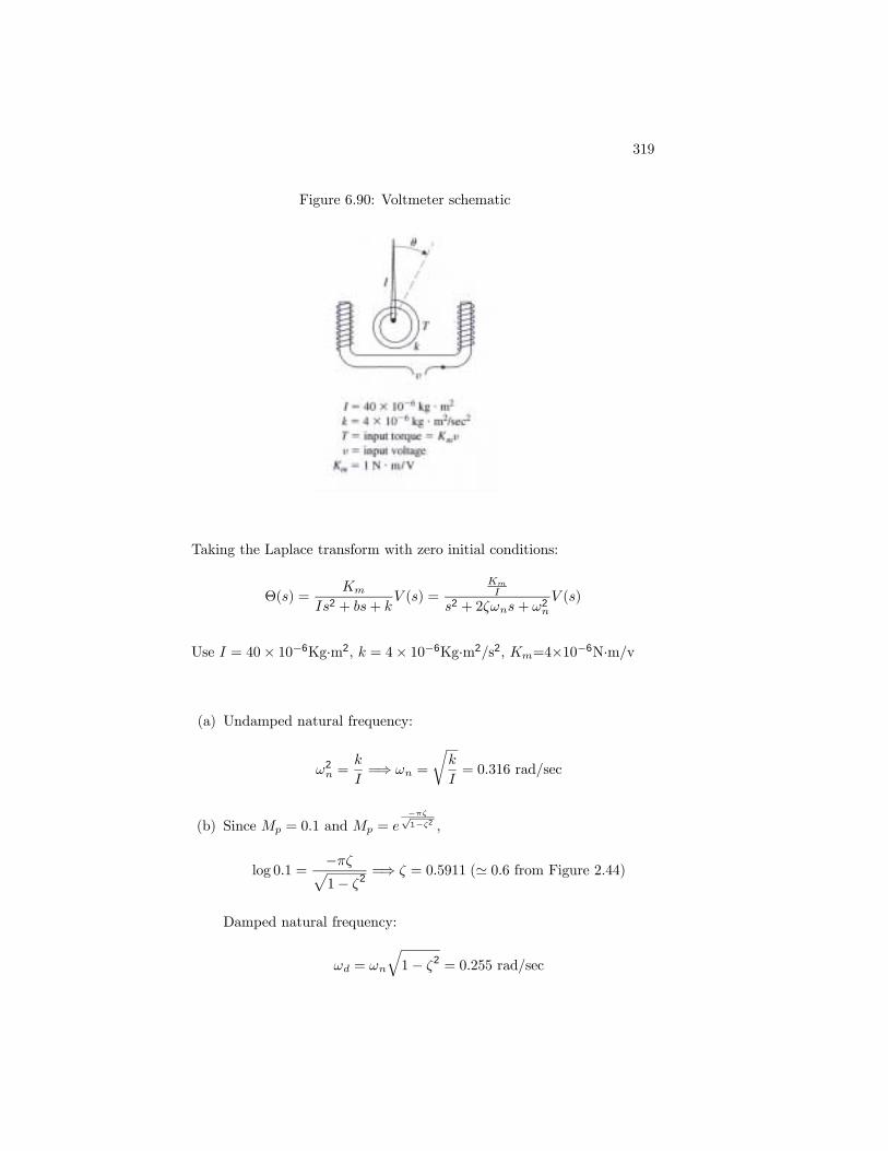
Figure 6.90: Voltmeter schematic
Taking the Laplace transform with zero initial conditions:
Θ(s) =Km
Is2 + bs+ kV (s) =
Km
I
s2 + 2ζωns+ ω2n
V (s)
Use I = 40× 10−6Kg·m2, k = 4× 10⁻⁶Kg·m2/s2, Km=4×10⁻⁶N·m/v
(a) Undamped natural frequency:
ω2n =
k
I=⇒ ωn =
rk
I= 0.316 rad/sec
(b) Since Mp = 0.1 and Mp = e−πζ√1−ζ2 ,
log 0.1 =−πζp1− ζ2
=⇒ ζ = 0.5911 (' 0.6 from Figure 2.44)
Damped natural frequency:
ωd = ωn
q1− ζ2 = 0.255 rad/sec
320 CHAPTER 6. THE FREQUENCY-RESPONSE DESIGN METHOD
(c)
T (jω) =Θ(jω)
V (jω)=
Km/I
(jω)2 + 2ζωnjω + ω2n
|T (jω)| =Km/I
[(ω2n − ω2)2 + (2ζωnω)2]
12
d |T (jω)|dω
=
µKmI
¶2ω©ω2n − ω2 − 2ζ2ω2
n
ª[(ω2
n − ω2)2 + (2ζωnω)2]32
When d|T (jω)|dω = 0,
ω2 − (1− 2ζ2)ω2n = 0
ω = 0.549ωn = 0.173
Alternatively, the peak frequency can be found from the Bode plot:
ω = 0.173 rad/sec
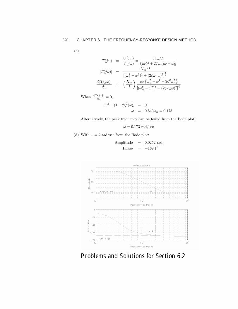
(d) With ω = 2 rad/sec from the Bode plot:
Amplitude = 0.0252 rad
Phase = −169.1
10-1
100
101
10-2
10-1
100
Frequency (rad/sec)
Magnitude
B ode D iagram s
|G (jw )|=0.025 w =2
10-1
100
101
-200
-150
-100
-50
0
Frequency (rad/sec)
Phase (deg)
-169 (deg)
w =2
Problems and Solutions for Section 6.2
321
16. Determine the range of K for which each of the following systems is stableby making a Bode plot for K = 1 and imagining the magnitude plotsliding up or down until instability results. Verify your answers using avery rough sketch of a root-locus plot.
(a) KG(s) =K(s+ 2)
s+ 20
(b) KG(s) =K
(s+ 10)(s+ 1)2
(c) KG(s) =K(s+ 10)(s+ 1)
(s+ 100)(s+ 5)3
Solution :
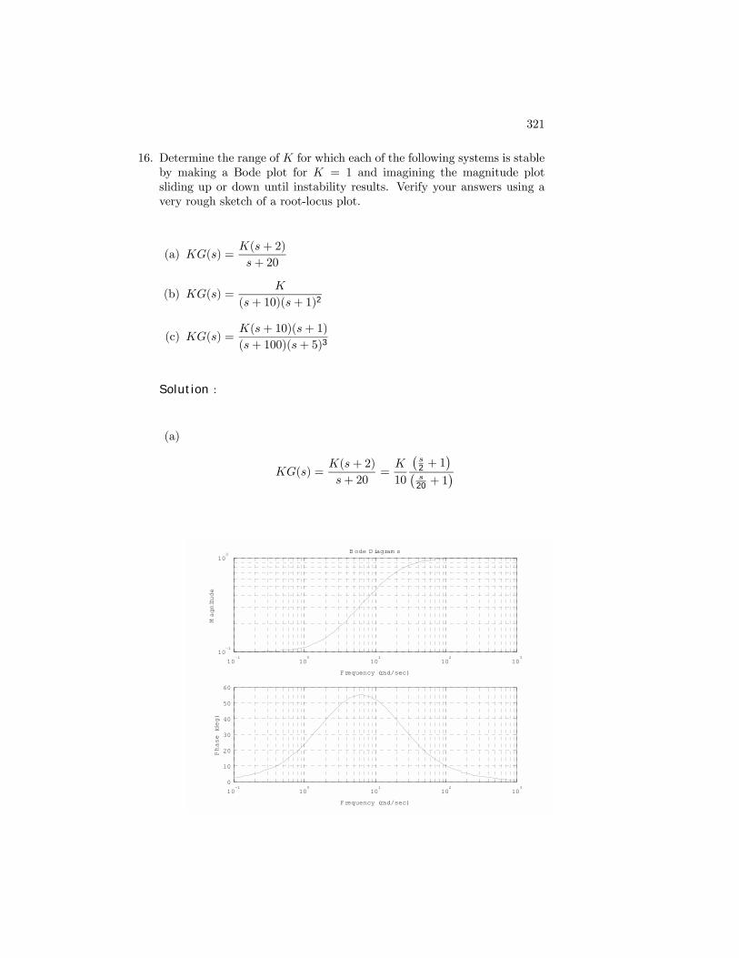
(a)
KG(s) =K(s+ 2)
s+ 20=K
10
¡s2 + 1
¢¡s
20 + 1¢
10-1
100
101
102
103
10-1
100
Frequency (rad/sec)
Magnitude
B ode D iagram s
10-1
100
101
102
103
0
10
20
30
40
50
60
Frequency (rad/sec)
Phase (deg)
322 CHAPTER 6. THE FREQUENCY-RESPONSE DESIGN METHOD
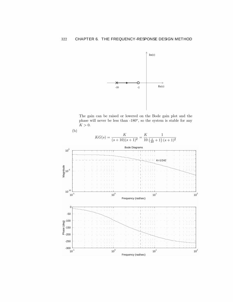
The gain can be raised or lowered on the Bode gain plot and thephase will never be less than -180o, so the system is stable for anyK > 0.
(b)
KG(s) =K
(s+ 10)(s+ 1)2=K
10
1¡s
10 + 1¢(s+ 1)2
10-1 100 101 10210-10
10-5
100
Frequency (rad/sec)
Mag
nitu
de
Bode Diagrams
K=1/242
10-1 100 101 102-300
-250
-200
-150
-100
-50
0
Frequency (rad/sec)
Phas
e (d
eg)
323
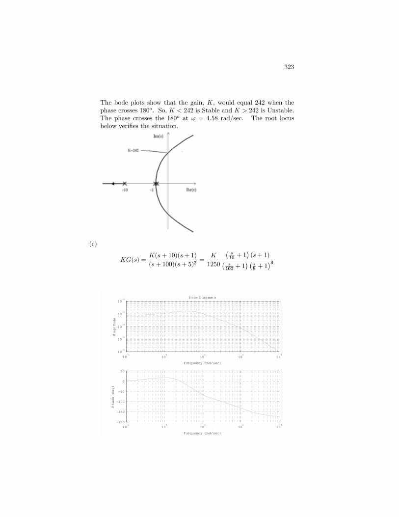
The bode plots show that the gain, K, would equal 242 when thephase crosses 180o. So, K < 242 is Stable and K > 242 is Unstable.The phase crosses the 180o at ω = 4.58 rad/sec. The root locusbelow veriÞes the situation.
(c)
KG(s) =K(s+ 10)(s+ 1)
(s+ 100)(s+ 5)3=
K
1250
¡s
10 + 1¢(s+ 1)¡
s100 + 1
¢ ¡s5 + 1
¢3
10-1
100
101
102
103
10-6
10-5
10-4
10-3
10-2
Frequency (rad/sec)
Magnitude
B ode D iagram s
10-1
100
101
102
103
-200
-150
-100
-50
0
50
Frequency (rad/sec)
Phase (deg)
324 CHAPTER 6. THE FREQUENCY-RESPONSE DESIGN METHOD
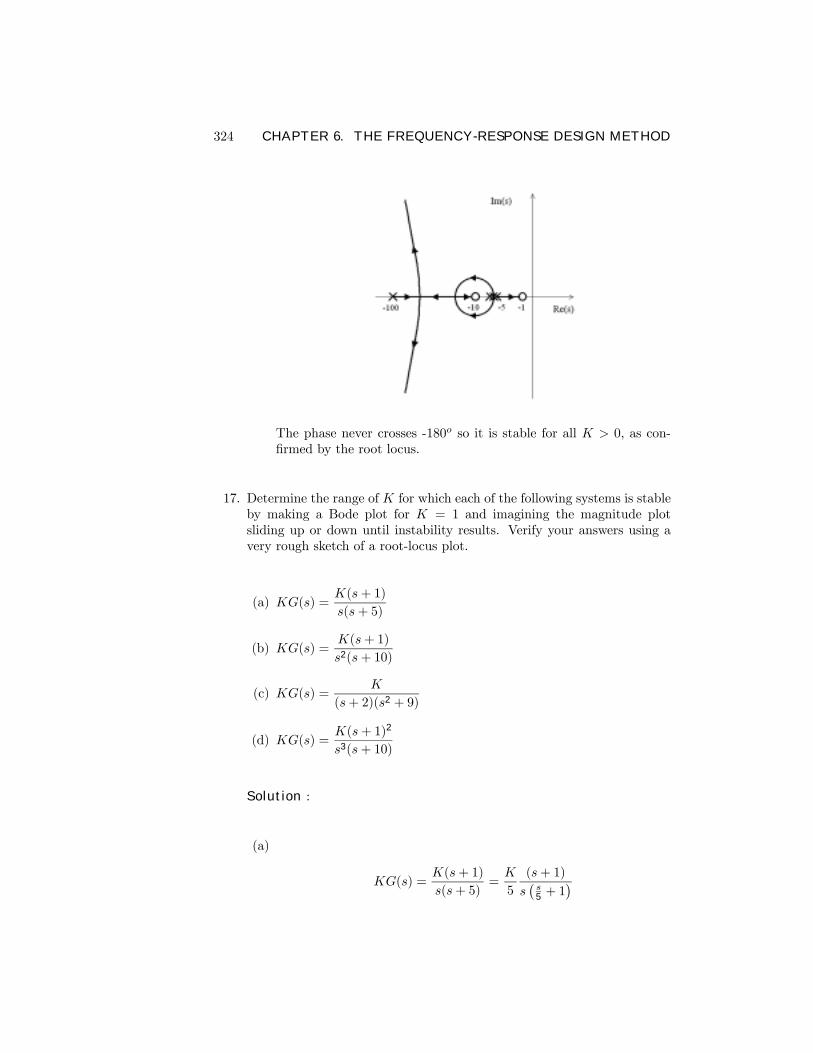
The phase never crosses -180o so it is stable for all K > 0, as con-Þrmed by the root locus.
17. Determine the range of K for which each of the following systems is stableby making a Bode plot for K = 1 and imagining the magnitude plotsliding up or down until instability results. Verify your answers using avery rough sketch of a root-locus plot.
(a) KG(s) =K(s+ 1)
s(s+ 5)
(b) KG(s) =K(s+ 1)
s2(s+ 10)
(c) KG(s) =K
(s+ 2)(s2 + 9)
(d) KG(s) =K(s+ 1)2
s3(s+ 10)
Solution :
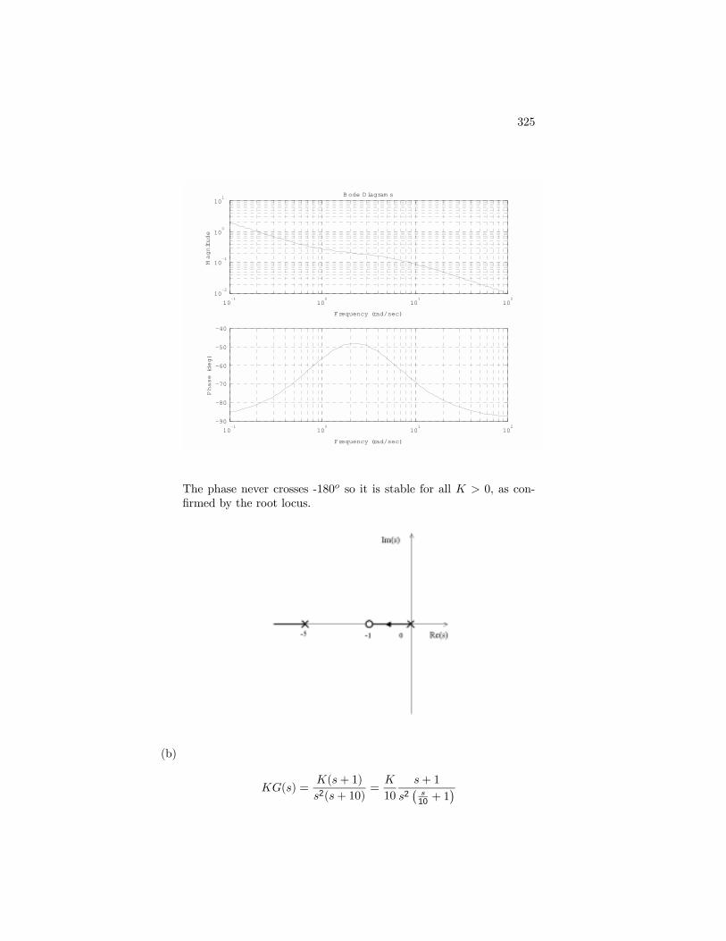
(a)
KG(s) =K(s+ 1)
s(s+ 5)=K
5
(s+ 1)
s¡s5 + 1
¢
325
10-1
100
101
102
10-2
10-1
100
101
Frequency (rad/sec)
Magnitude
B ode D iagram s
10-1
100
101
102
-90
-80
-70
-60
-50
-40
Frequency (rad/sec)
Phase (deg)
The phase never crosses -180o so it is stable for all K > 0, as con-Þrmed by the root locus.
(b)
KG(s) =K(s+ 1)
s2(s+ 10)=K
10
s+ 1
s2¡s
10 + 1¢
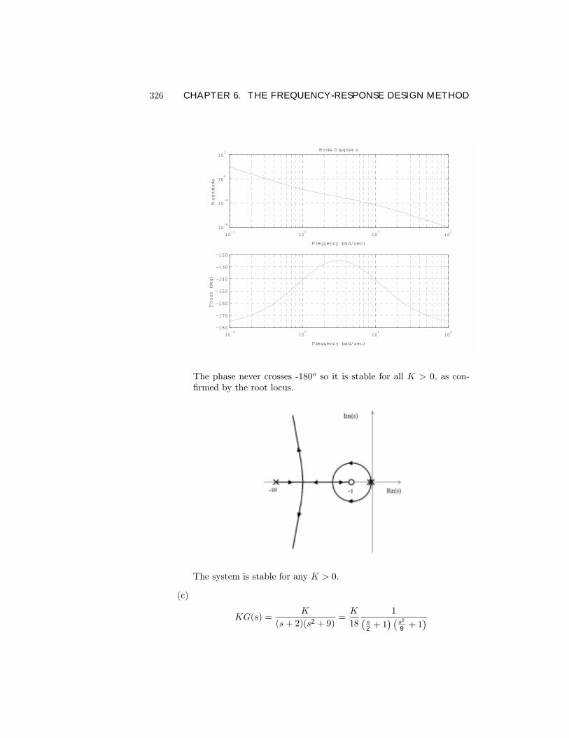
326 CHAPTER 6. THE FREQUENCY-RESPONSE DESIGN METHOD
10-1
100
101
102
10-4
10-2
100
102
Frequency (rad/sec)
Magnitude
B ode D iagram s
10-1
100
101
102
-180
-170
-160
-150
-140
-130
-120
Frequency (rad/sec)
Phase (deg)
The phase never crosses -180o so it is stable for all K > 0, as con-Þrmed by the root locus.
The system is stable for any K > 0.
(c)
KG(s) =K
(s+ 2)(s2 + 9)=K
18
1¡s2 + 1
¢ ¡s2
9 + 1¢
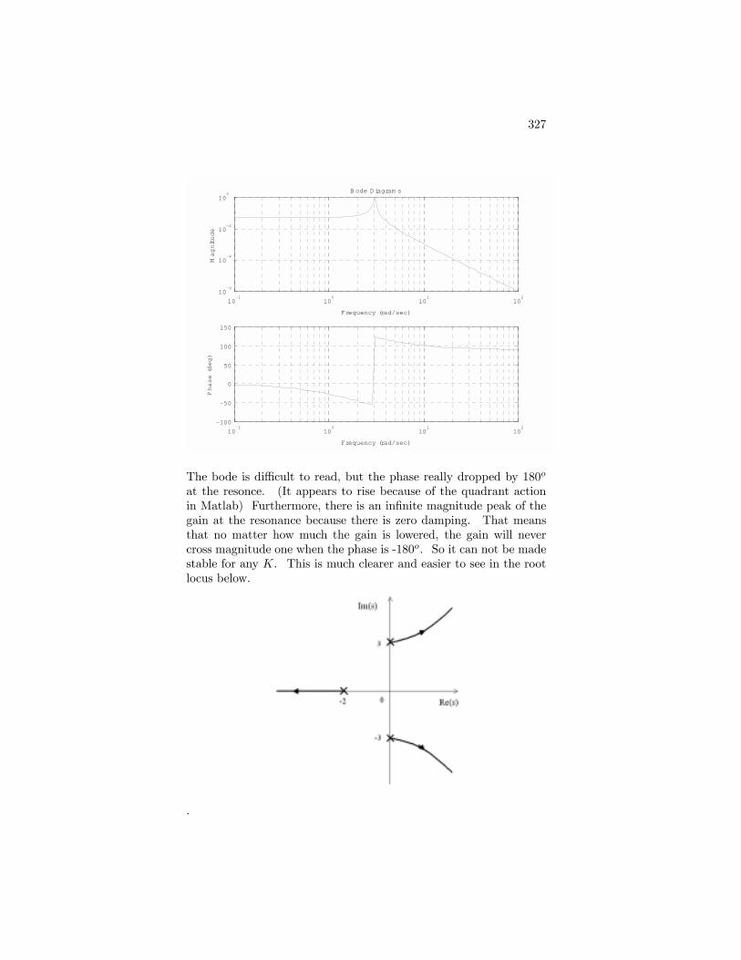
327
10-1
100
101
102
10-6
10-4
10-2
100
Frequency (rad/sec)
Magnitude
B ode D iagram s
10-1
100
101
102
-100
-50
0
50
100
150
Frequency (rad/sec)
Phase (deg)
The bode is difficult to read, but the phase really dropped by 180o
at the resonce. (It appears to rise because of the quadrant actionin Matlab) Furthermore, there is an inÞnite magnitude peak of thegain at the resonance because there is zero damping. That meansthat no matter how much the gain is lowered, the gain will nevercross magnitude one when the phase is -180o. So it can not be madestable for any K. This is much clearer and easier to see in the rootlocus below.
.
328 CHAPTER 6. THE FREQUENCY-RESPONSE DESIGN METHOD
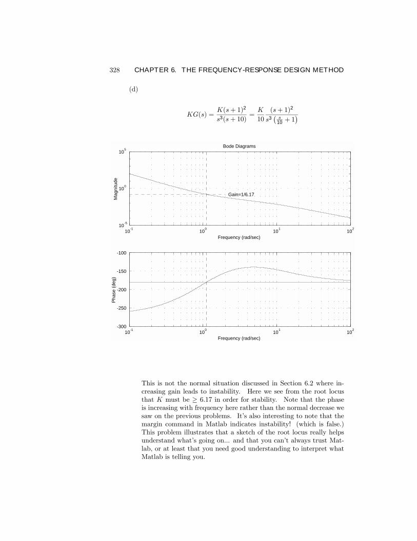
(d)
KG(s) =K(s+ 1)2
s3(s+ 10)=K
10
(s+ 1)2
s3¡s
10 + 1¢
10-1 100 101 10210-5
100
105
Frequency (rad/sec)
Mag
nitu
de
Bode Diagrams
Gain=1/6.17
10-1 100 101 102-300
-250
-200
-150
-100
Frequency (rad/sec)
Phas
e (d
eg)
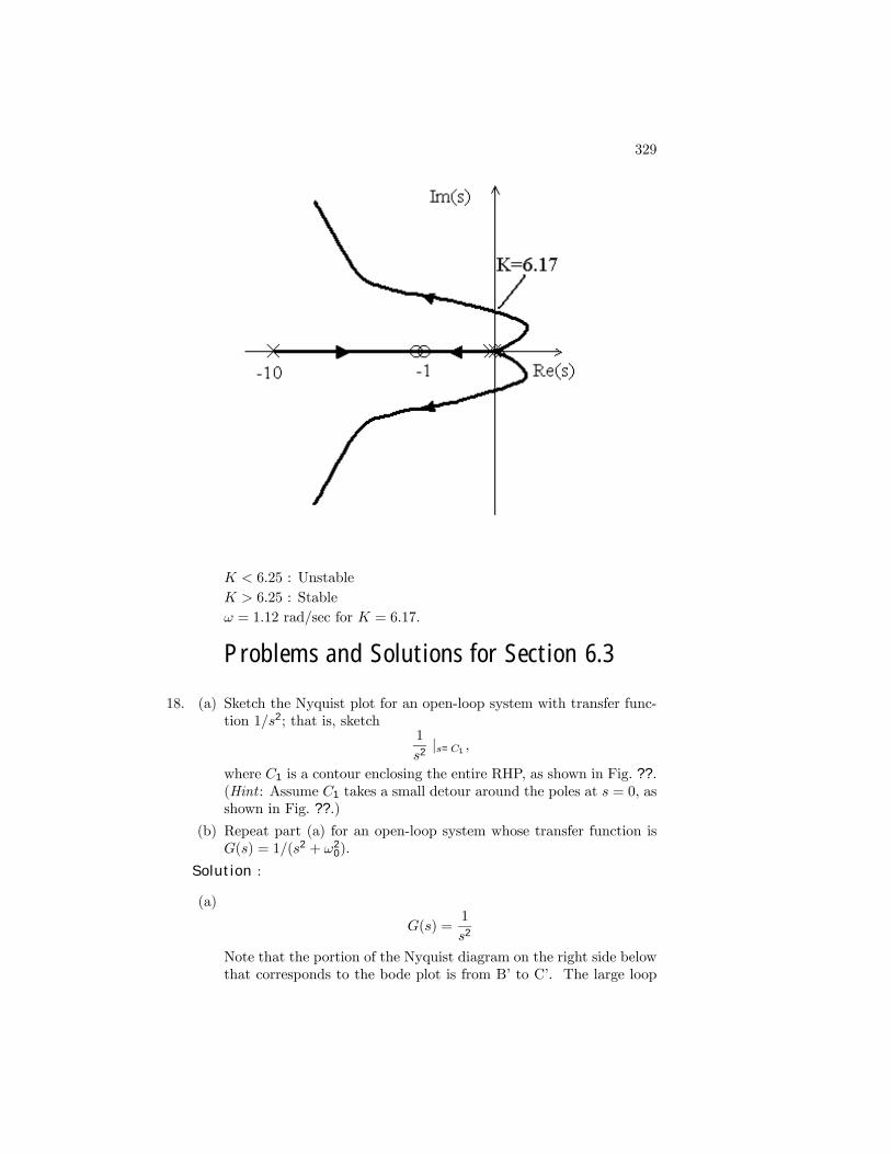
This is not the normal situation discussed in Section 6.2 where in-creasing gain leads to instability. Here we see from the root locusthat K must be ≥ 6.17 in order for stability. Note that the phaseis increasing with frequency here rather than the normal decrease wesaw on the previous problems. Its also interesting to note that themargin command in Matlab indicates instability! (which is false.)This problem illustrates that a sketch of the root locus really helpsunderstand whats going on... and that you cant always trust Mat-lab, or at least that you need good understanding to interpret whatMatlab is telling you.
329
K < 6.25 : Unstable
K > 6.25 : Stable
ω = 1.12 rad/sec for K = 6.17.
Problems and Solutions for Section 6.3
18. (a) Sketch the Nyquist plot for an open-loop system with transfer func-tion 1/s2; that is, sketch
1
s2|s=C1 ,
where C1 is a contour enclosing the entire RHP, as shown in Fig. ??.(Hint : Assume C1 takes a small detour around the poles at s = 0, asshown in Fig. ??.)
(b) Repeat part (a) for an open-loop system whose transfer function isG(s) = 1/(s2 + ω2
0).
Solution :
(a)
G(s) =1
s2
Note that the portion of the Nyquist diagram on the right side belowthat corresponds to the bode plot is from B to C. The large loop
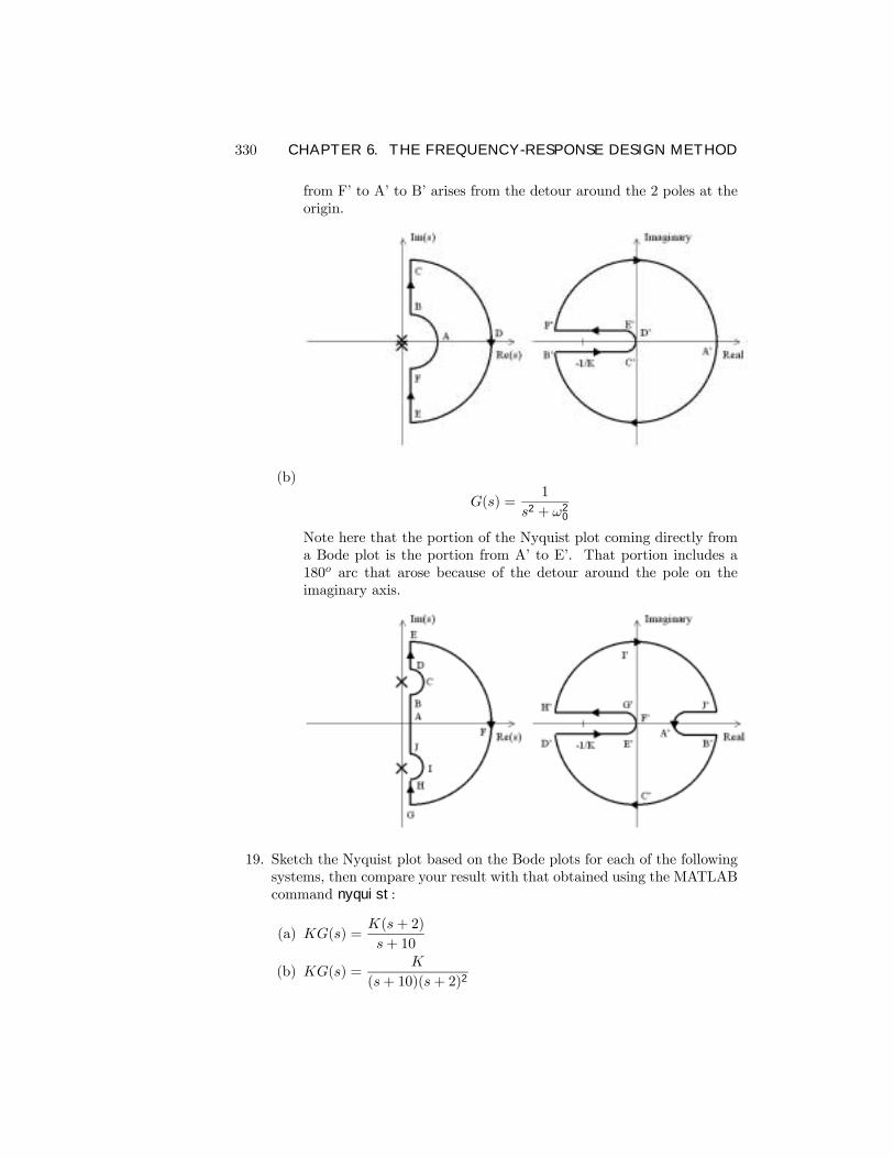
330 CHAPTER 6. THE FREQUENCY-RESPONSE DESIGN METHOD
from F to A to B arises from the detour around the 2 poles at theorigin.
(b)
G(s) =1
s2 + ω20
Note here that the portion of the Nyquist plot coming directly froma Bode plot is the portion from A to E. That portion includes a180o arc that arose because of the detour around the pole on theimaginary axis.
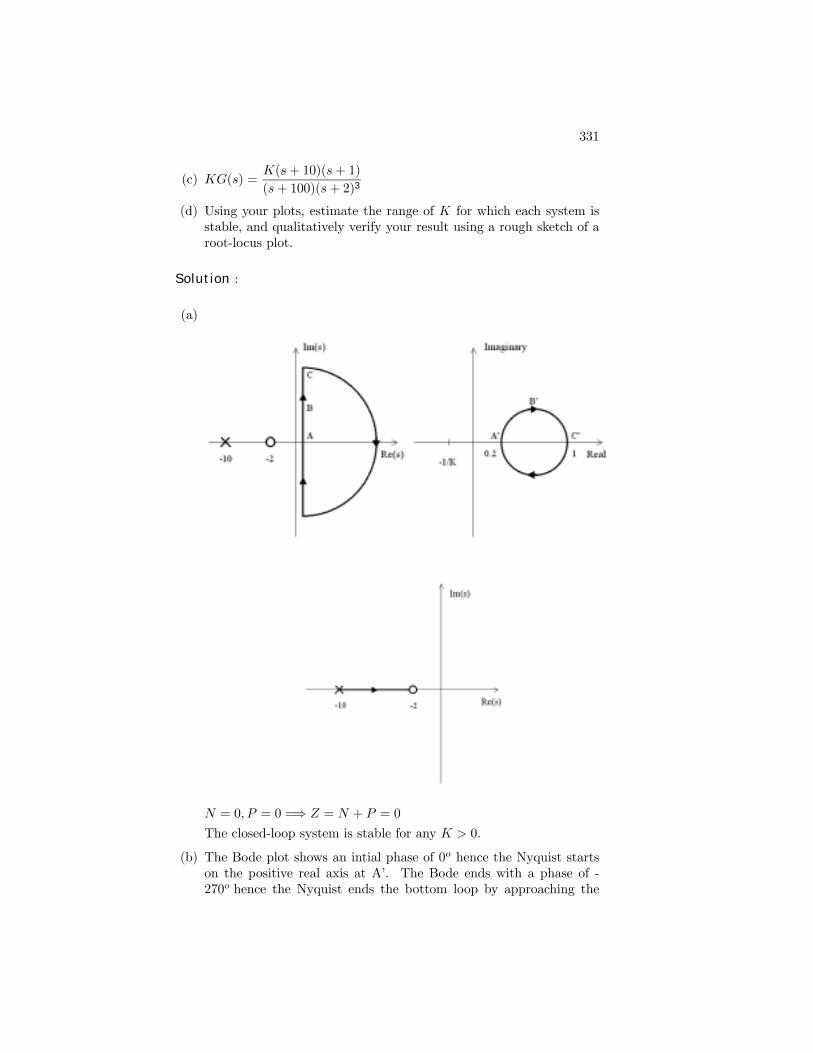
19. Sketch the Nyquist plot based on the Bode plots for each of the followingsystems, then compare your result with that obtained using the MATLABcommand nyquist:
(a) KG(s) =K(s+ 2)
s+ 10
(b) KG(s) =K
(s+ 10)(s+ 2)2
331
(c) KG(s) =K(s+ 10)(s+ 1)
(s+ 100)(s+ 2)3
(d) Using your plots, estimate the range of K for which each system isstable, and qualitatively verify your result using a rough sketch of aroot-locus plot.
Solution :
(a)
N = 0, P = 0 =⇒ Z = N + P = 0
The closed-loop system is stable for any K > 0.
(b) The Bode plot shows an intial phase of 0o hence the Nyquist startson the positive real axis at A. The Bode ends with a phase of -270o hence the Nyquist ends the bottom loop by approaching the
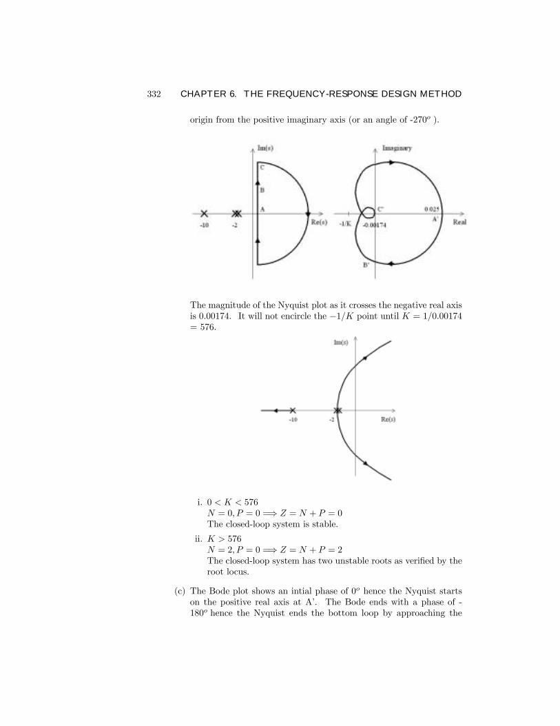
332 CHAPTER 6. THE FREQUENCY-RESPONSE DESIGN METHOD
origin from the positive imaginary axis (or an angle of -270o ).
The magnitude of the Nyquist plot as it crosses the negative real axisis 0.00174. It will not encircle the −1/K point until K = 1/0.00174= 576.
i. 0 < K < 576N = 0, P = 0 =⇒ Z = N + P = 0The closed-loop system is stable.
ii. K > 576N = 2, P = 0 =⇒ Z = N + P = 2The closed-loop system has two unstable roots as veriÞed by theroot locus.
(c) The Bode plot shows an intial phase of 0o hence the Nyquist startson the positive real axis at A. The Bode ends with a phase of -180o hence the Nyquist ends the bottom loop by approaching the
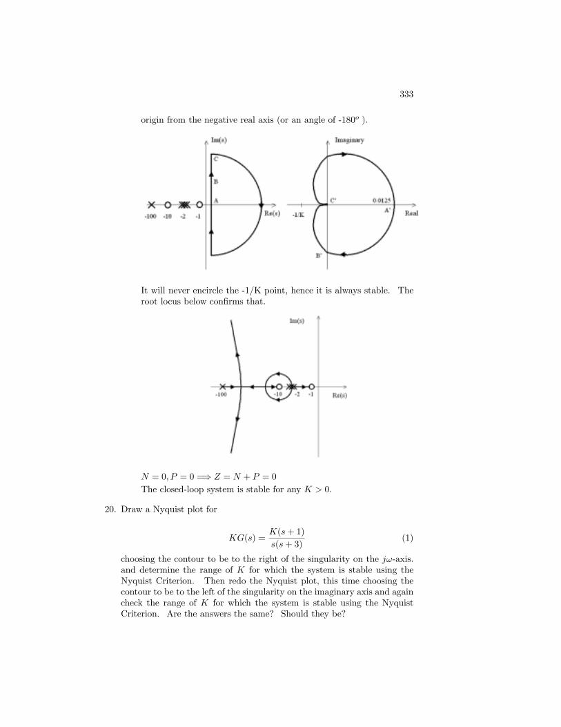
333
origin from the negative real axis (or an angle of -180o ).
It will never encircle the -1/K point, hence it is always stable. Theroot locus below conÞrms that.
N = 0, P = 0 =⇒ Z = N + P = 0
The closed-loop system is stable for any K > 0.
20. Draw a Nyquist plot for
KG(s) =K(s+ 1)
s(s+ 3)(1)
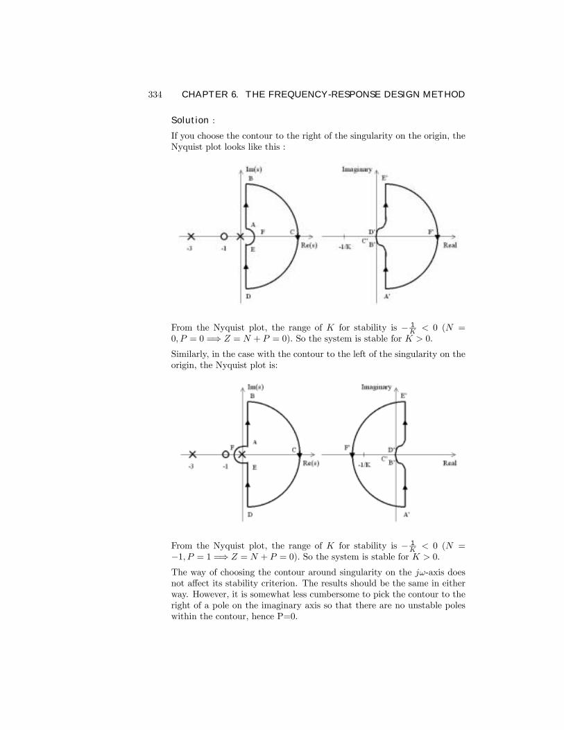
choosing the contour to be to the right of the singularity on the jω-axis.and determine the range of K for which the system is stable using theNyquist Criterion. Then redo the Nyquist plot, this time choosing thecontour to be to the left of the singularity on the imaginary axis and againcheck the range of K for which the system is stable using the NyquistCriterion. Are the answers the same? Should they be?
334 CHAPTER 6. THE FREQUENCY-RESPONSE DESIGN METHOD
Solution :
If you choose the contour to the right of the singularity on the origin, theNyquist plot looks like this :
From the Nyquist plot, the range of K for stability is − 1K < 0 (N =
0, P = 0 =⇒ Z = N + P = 0). So the system is stable for K > 0.
Similarly, in the case with the contour to the left of the singularity on theorigin, the Nyquist plot is:
From the Nyquist plot, the range of K for stability is − 1K < 0 (N =
−1, P = 1 =⇒ Z = N + P = 0). So the system is stable for K > 0.
The way of choosing the contour around singularity on the jω-axis doesnot affect its stability criterion. The results should be the same in eitherway. However, it is somewhat less cumbersome to pick the contour to theright of a pole on the imaginary axis so that there are no unstable poleswithin the contour, hence P=0.
335
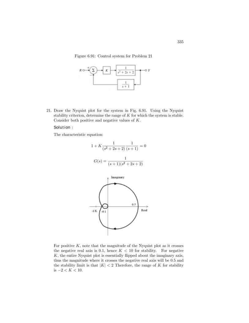
Figure 6.91: Control system for Problem 21
21. Draw the Nyquist plot for the system in Fig. 6.91. Using the Nyquiststability criterion, determine the range ofK for which the system is stable.Consider both positive and negative values of K.
Solution :
The characteristic equation:
1 +K1
(s2 + 2s+ 2)
1
(s+ 1)= 0
G(s) =1
(s+ 1)(s2 + 2s+ 2)
For positive K, note that the magnitude of the Nyquist plot as it crossesthe negative real axis is 0.1, hence K < 10 for stability. For negativeK, the entire Nyquist plot is essentially ßipped about the imaginary axis,thus the magnitude where it crosses the negative real axis will be 0.5 andthe stability limit is that |K| < 2 Therefore, the range of K for stabilityis −2 < K < 10.
336 CHAPTER 6. THE FREQUENCY-RESPONSE DESIGN METHOD
22. (a) For ω = 0.1 to 100 rad/sec, sketch the phase of the minimum-phasesystem
¯G(s) =
s+ 1
s+ 10
¯s=jω
and the nonminimum-phase system
¯G(s) = − s− 1
s+ 10
¯s=jω
,
noting that ∠(jω − 1) decreases with ω rather than increasing.
(b) Does a RHP zero affect the relationship between the−1 encirclementson a polar plot and the number of unstable closed-loop roots inEq. (6.28)?
(c) Sketch the phase of the following unstable system for ω = 0.1 to100 rad/sec:
G(s) =
¯s+ 1
s− 10¯s=jω
.
(d) Check the stability of the systems in (a) and (c) using the Nyquistcriterion on KG(s). Determine the range of K for which the closed-loop system is stable, and check your results qualitatively using arough root-locus sketch.
Solution :
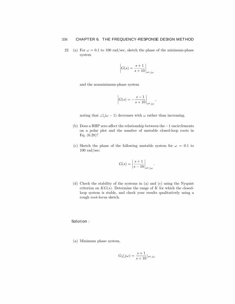
(a) Minimum phase system,
G1(jω) =s+ 1
s+ 10|s=jω
337
10-1
100
101
102
10-1
100
Frequency (rad/sec)
Magnitude
B ode D iagram s
10-1
100
101
102
0
20
40
60
80
100
Frequency (rad/sec)
Phase (deg)
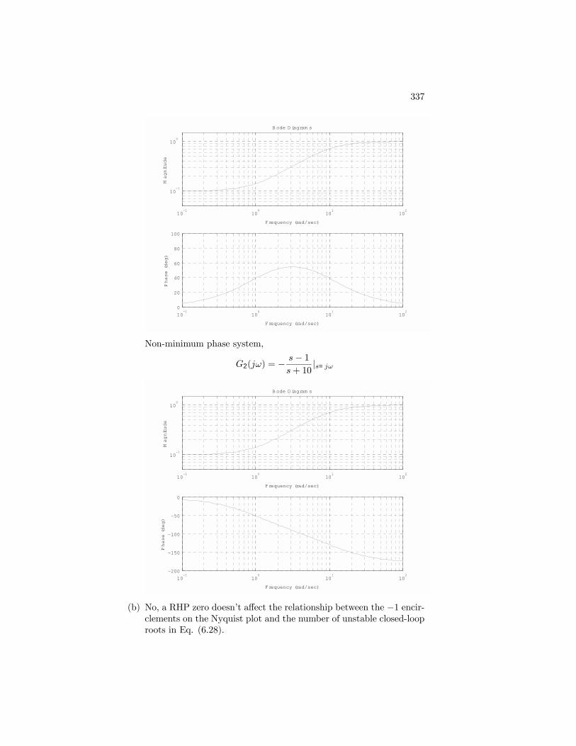
Non-minimum phase system,
G2(jω) = − s− 1s+ 10
|s=jω
10-1
100
101
102
10-1
100
Frequency (rad/sec)
Magnitude
B ode D iagram s
10-1
100
101
102
-200
-150
-100
-50
0
Frequency (rad/sec)
Phase (deg)
(b) No, a RHP zero doesnt affect the relationship between the −1 encir-clements on the Nyquist plot and the number of unstable closed-looproots in Eq. (6.28).
338 CHAPTER 6. THE FREQUENCY-RESPONSE DESIGN METHOD
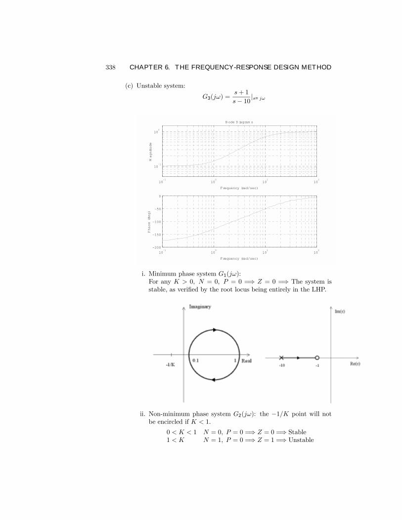
(c) Unstable system:
G3(jω) =s+ 1
s− 10 |s=jω
10-1
100
101
102
10-1
100
Frequency (rad/sec)
Magnitude
B ode D iagram s
10-1
100
101
102
-200
-150
-100
-50
0
Frequency (rad/sec)
Phase (deg)
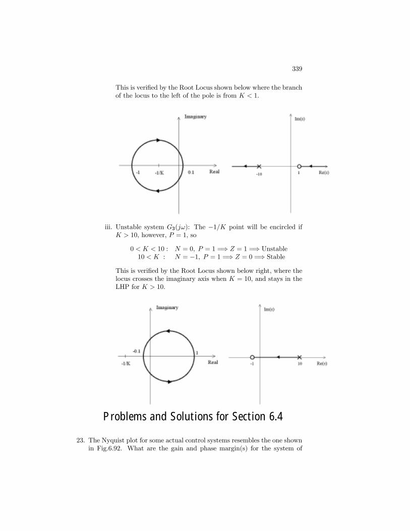
i. Minimum phase system G1(jω):For any K > 0, N = 0, P = 0 =⇒ Z = 0 =⇒ The system isstable, as veriÞed by the root locus being entirely in the LHP.
ii. Non-minimum phase system G2(jω): the −1/K point will notbe encircled if K < 1.
0 < K < 1 N = 0, P = 0 =⇒ Z = 0 =⇒ Stable1 < K N = 1, P = 0 =⇒ Z = 1 =⇒ Unstable
339
This is veriÞed by the Root Locus shown below where the branchof the locus to the left of the pole is from K < 1.
iii. Unstable system G3(jω): The −1/K point will be encircled ifK > 10, however, P = 1, so
0 < K < 10 : N = 0, P = 1 =⇒ Z = 1 =⇒ Unstable10 < K : N = −1, P = 1 =⇒ Z = 0 =⇒ Stable
This is veriÞed by the Root Locus shown below right, where thelocus crosses the imaginary axis when K = 10, and stays in theLHP for K > 10.
Problems and Solutions for Section 6.4
23. The Nyquist plot for some actual control systems resembles the one shownin Fig.6.92. What are the gain and phase margin(s) for the system of
340 CHAPTER 6. THE FREQUENCY-RESPONSE DESIGN METHOD
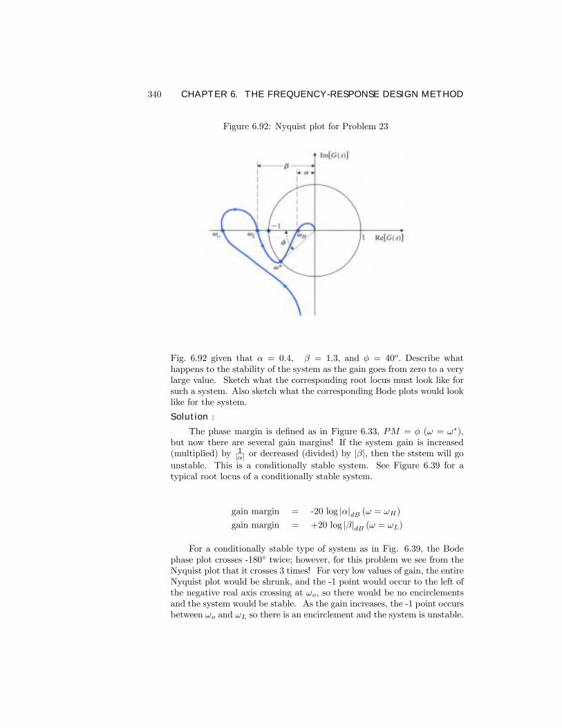
Figure 6.92: Nyquist plot for Problem 23
Fig. 6.92 given that α = 0.4, β = 1.3, and φ = 40o. Describe whathappens to the stability of the system as the gain goes from zero to a verylarge value. Sketch what the corresponding root locus must look like forsuch a system. Also sketch what the corresponding Bode plots would looklike for the system.
Solution :
The phase margin is deÞned as in Figure 6.33, PM = φ (ω = ω∗),but now there are several gain margins! If the system gain is increased(multiplied) by 1
|α| or decreased (divided) by |β|, then the ststem will go
unstable. This is a conditionally stable system. See Figure 6.39 for atypical root locus of a conditionally stable system.
gain margin = -20 log |α|dB (ω = ωH)gain margin = +20 log |β|dB (ω = ωL)
For a conditionally stable type of system as in Fig. 6.39, the Bodephase plot crosses -180 twice; however, for this problem we see from theNyquist plot that it crosses 3 times! For very low values of gain, the entireNyquist plot would be shrunk, and the -1 point would occur to the left ofthe negative real axis crossing at ωo, so there would be no encirclementsand the system would be stable. As the gain increases, the -1 point occursbetween ωo and ωL so there is an encirclement and the system is unstable.
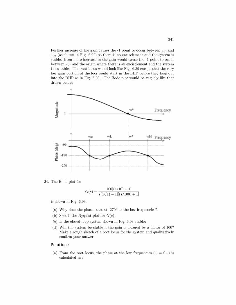
341
Further increase of the gain causes the -1 point to occur between ωL andωH (as shown in Fig. 6.92) so there is no encirclement and the system isstable. Even more increase in the gain would cause the -1 point to occurbetween ωH and the origin where there is an encirclement and the systemis unstable. The root locus would look like Fig. 6.39 except that the verylow gain portion of the loci would start in the LHP before they loop outinto the RHP as in Fig. 6.39. The Bode plot would be vaguely like thatdrawn below:
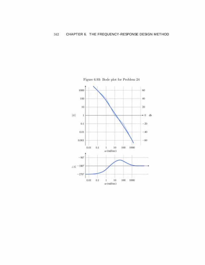
24. The Bode plot for
G(s) =100[(s/10) + 1]
s[(s/1)− 1][(s/100) + 1]is shown in Fig. 6.93.
(a) Why does the phase start at -270o at the low frequencies?
(b) Sketch the Nyquist plot for G(s).
(c) Is the closed-loop system shown in Fig. 6.93 stable?
(d) Will the system be stable if the gain is lowered by a factor of 100?Make a rough sketch of a root locus for the system and qualitativelyconÞrm your answer
Solution :
(a) From the root locus, the phase at the low frequencies (ω = 0+) iscalculated as :
342 CHAPTER 6. THE FREQUENCY-RESPONSE DESIGN METHOD
Figure 6.93: Bode plot for Problem 24
343
The phase at the point s = jω(ω = 0+)= −180(pole : s = 1)− 90(pole : s = 0) + 0(zero : s = −10) + 0(pole : s = −100)= −270
Or, more simply, the RHP pole at s = +1 causes a −180o shift fromthe −90o that you would expect from a normal system with all thesingularities in the LHP.
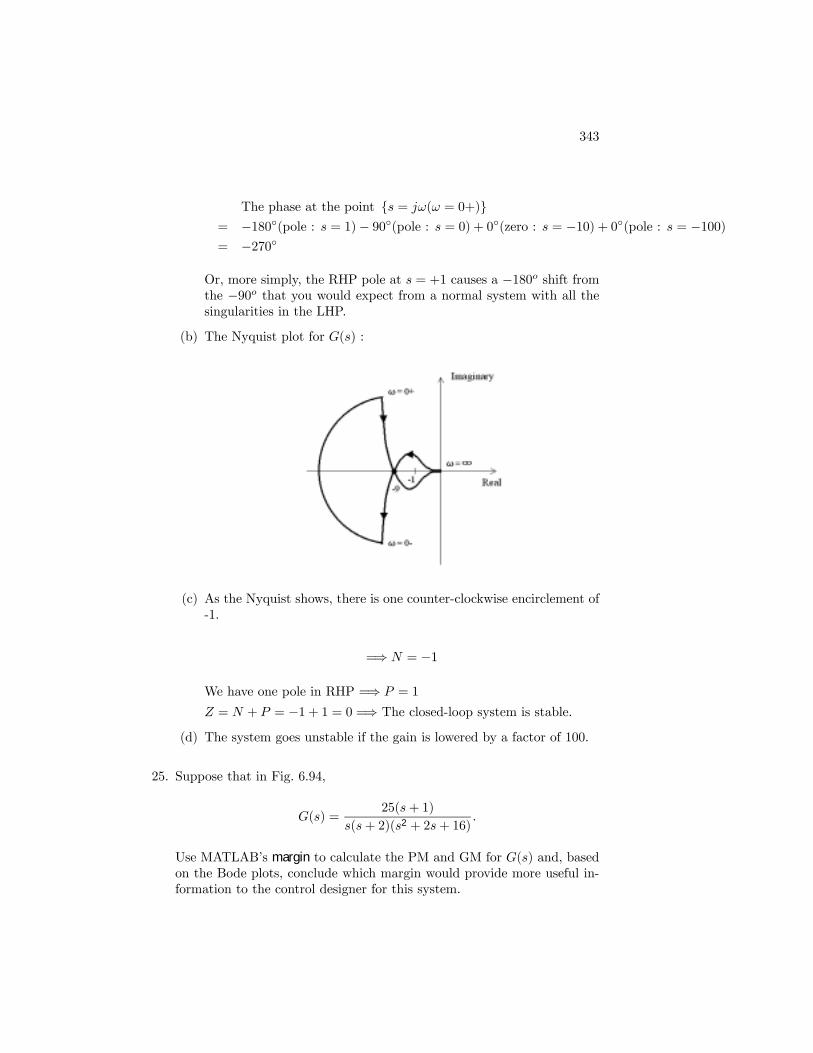
(b) The Nyquist plot for G(s) :
(c) As the Nyquist shows, there is one counter-clockwise encirclement of-1.
=⇒ N = −1
We have one pole in RHP =⇒ P = 1
Z = N + P = −1 + 1 = 0 =⇒ The closed-loop system is stable.
(d) The system goes unstable if the gain is lowered by a factor of 100.
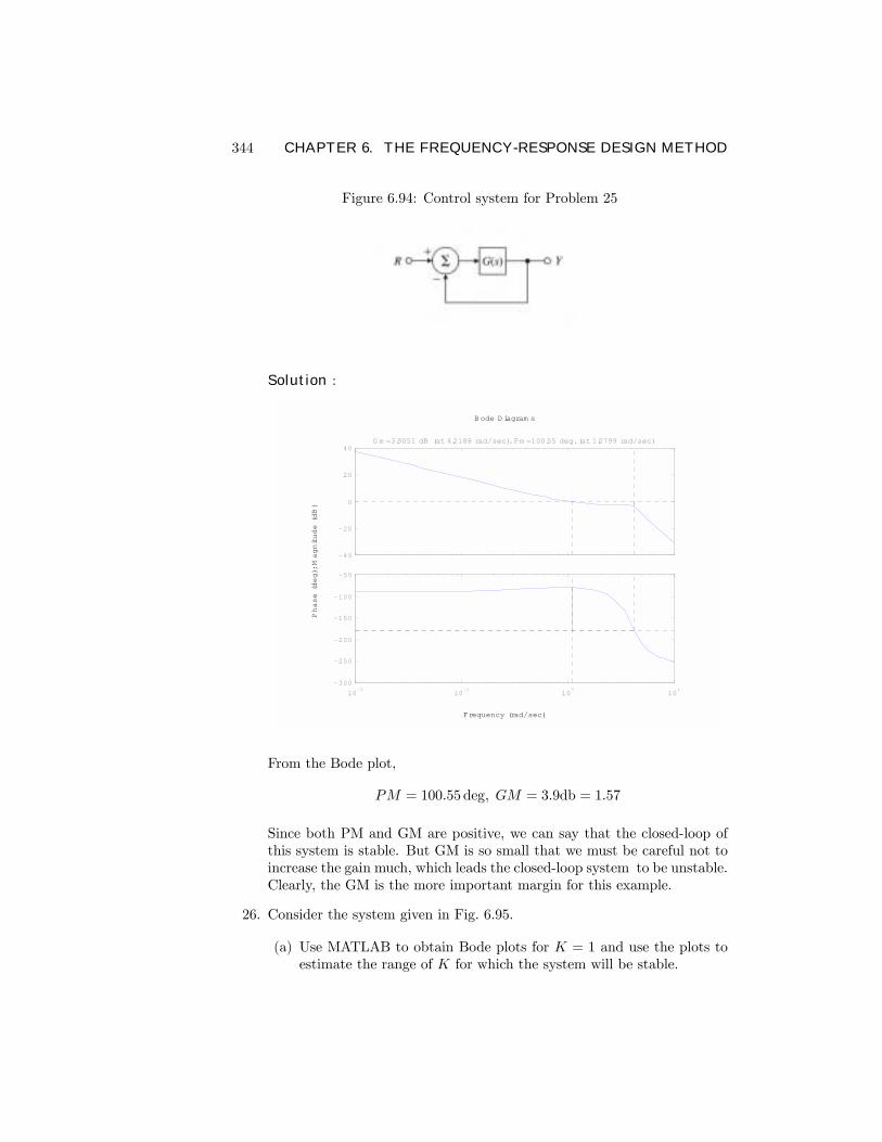
25. Suppose that in Fig. 6.94,
G(s) =25(s+ 1)
s(s+ 2)(s2 + 2s+ 16).
Use MATLABs margin to calculate the PM and GM for G(s) and, basedon the Bode plots, conclude which margin would provide more useful in-formation to the control designer for this system.
344 CHAPTER 6. THE FREQUENCY-RESPONSE DESIGN METHOD
Figure 6.94: Control system for Problem 25
Solution :
Frequency (rad/sec)
Phase (deg); M
agnitude (dB)
B ode D iagram s
-40
-20
0
20
40G m =3.9051 dB (at 4.2188 rad/sec), Pm =100.55 deg. (at 1.0799 rad/sec)
10-2
10-1
100
101
-300
-250
-200
-150
-100
-50
From the Bode plot,
PM = 100.55 deg, GM = 3.9db = 1.57
Since both PM and GM are positive, we can say that the closed-loop ofthis system is stable. But GM is so small that we must be careful not toincrease the gain much, which leads the closed-loop system to be unstable.Clearly, the GM is the more important margin for this example.
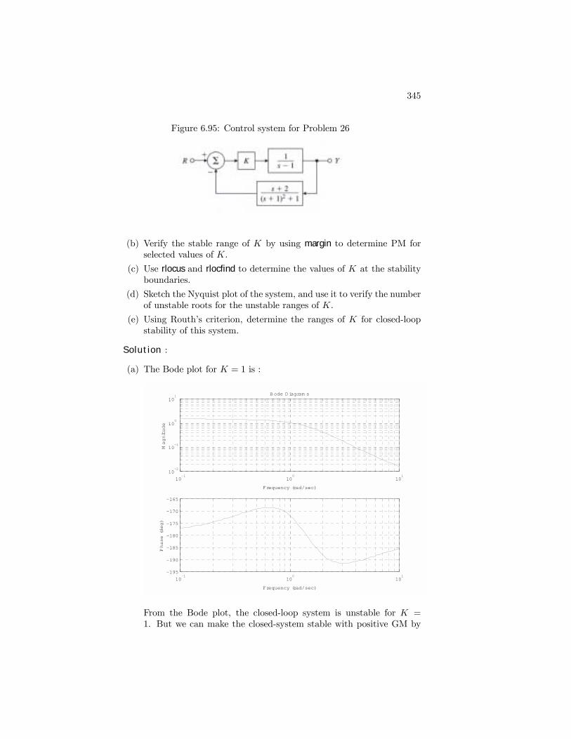
26. Consider the system given in Fig. 6.95.
(a) Use MATLAB to obtain Bode plots for K = 1 and use the plots toestimate the range of K for which the system will be stable.
345
Figure 6.95: Control system for Problem 26
(b) Verify the stable range of K by using margin to determine PM forselected values of K.
(c) Use rlocus and rlocfind to determine the values of K at the stabilityboundaries.
(d) Sketch the Nyquist plot of the system, and use it to verify the numberof unstable roots for the unstable ranges of K.
(e) Using Rouths criterion, determine the ranges of K for closed-loopstability of this system.
Solution :
(a) The Bode plot for K = 1 is :
10-1
100
101
10-2
10-1
100
101
Frequency (rad/sec)
Magnitude
B ode D iagram s
10-1
100
101
-195
-190
-185
-180
-175
-170
-165
Frequency (rad/sec)
Phase (deg)
From the Bode plot, the closed-loop system is unstable for K =1. But we can make the closed-system stable with positive GM by
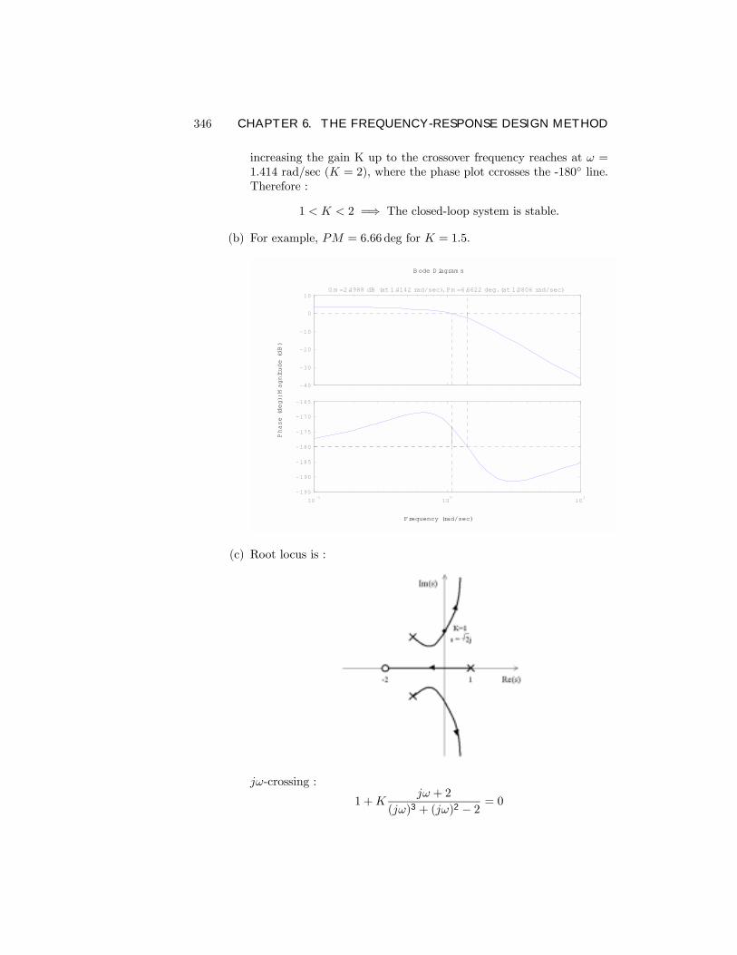
346 CHAPTER 6. THE FREQUENCY-RESPONSE DESIGN METHOD
increasing the gain K up to the crossover frequency reaches at ω =1.414 rad/sec (K = 2), where the phase plot ccrosses the -180 line.Therefore :
1 < K < 2 =⇒ The closed-loop system is stable.
(b) For example, PM = 6.66 deg for K = 1.5.
Frequency (rad/sec)
Phase (deg); M
agnitude (dB)
B ode D iagram s
-40
-30
-20
-10
0
10G m =2.4988 dB (at 1.4142 rad/sec), Pm =6.6622 deg. (at 1.0806 rad/sec)
10-1
100
101
-195
-190
-185
-180
-175
-170
-165
(c) Root locus is :
jω-crossing :
1 +Kjω + 2
(jω)3 + (jω)2 − 2 = 0
347
ω2 − 2K + 2 = 0
ω(ω2 −K) = 0
K = 2, ω = ±√2, or K = 1, ω = 0
Therefore,
1 < K < 2 =⇒ The closed-loop system is stable.
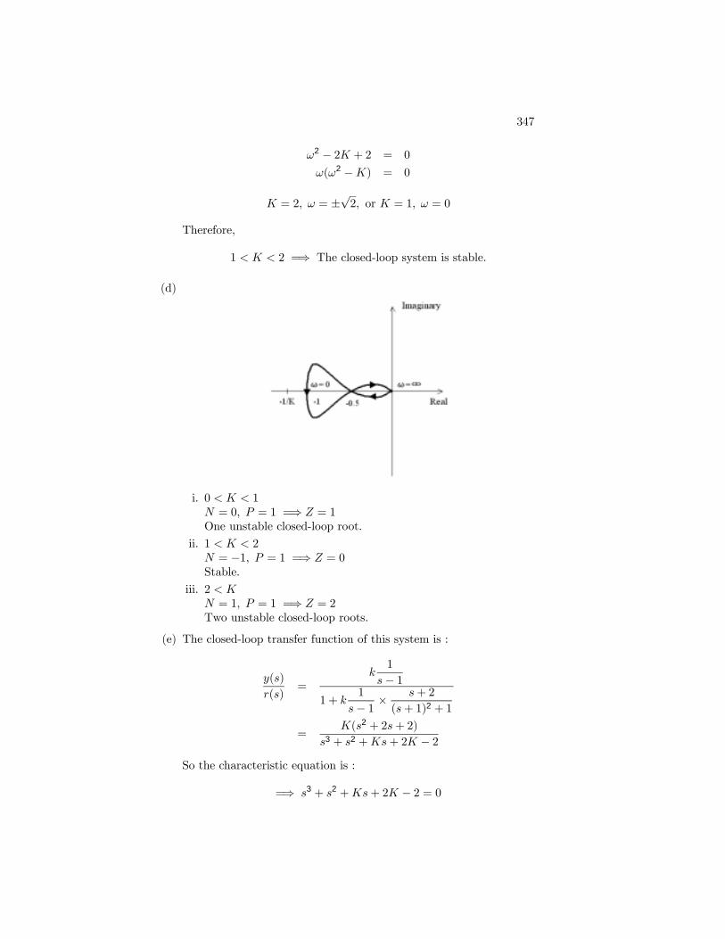
(d)
i. 0 < K < 1N = 0, P = 1 =⇒ Z = 1One unstable closed-loop root.
ii. 1 < K < 2N = −1, P = 1 =⇒ Z = 0Stable.
iii. 2 < KN = 1, P = 1 =⇒ Z = 2Two unstable closed-loop roots.
(e) The closed-loop transfer function of this system is :
y(s)
r(s)=
k1
s− 11 + k
1
s− 1 ×s+ 2
(s+ 1)2 + 1
=K(s2 + 2s+ 2)
s3 + s2 +Ks+ 2K − 2So the characteristic equation is :
=⇒ s3 + s2 +Ks+ 2K − 2 = 0
348 CHAPTER 6. THE FREQUENCY-RESPONSE DESIGN METHOD
Using the Rouths criterion,
s3 : 1 Ks2 : 1 2K − 2s1 : 2−K 0s0 : 2k = 2
For stability,
2−K > 0
2K − 2 > 0
=⇒ 2 > K > 1
0 < K < 1 Unstable1 < K < 2 Stable2 < K Unstable
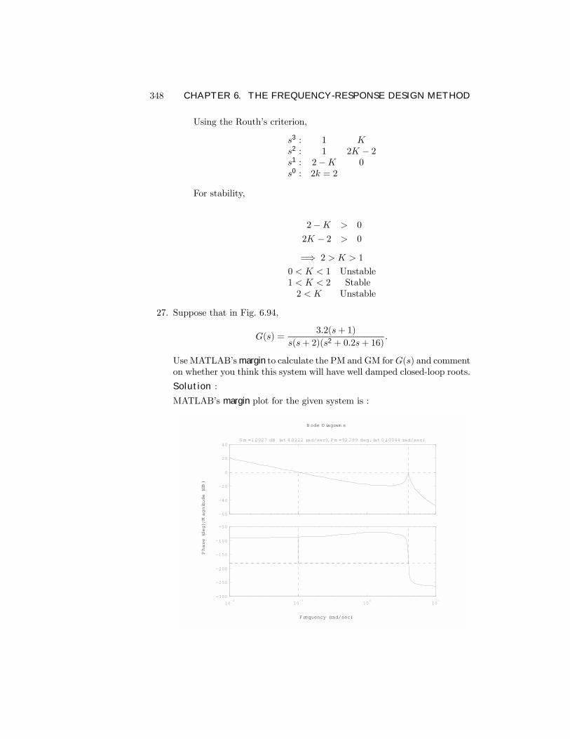
27. Suppose that in Fig. 6.94,
G(s) =3.2(s+ 1)
s(s+ 2)(s2 + 0.2s+ 16).
Use MATLABsmargin to calculate the PM and GM forG(s) and commenton whether you think this system will have well damped closed-loop roots.
Solution :
MATLABs margin plot for the given system is :
Frequency (rad/sec)
Phase (deg); M
agnitude (dB)
B ode D iagram s
-60
-40
-20
0
20
40G m =1.0027 dB (at 4.0222 rad/sec), Pm =92.789 deg. (at 0.10044 rad/sec)
10-2
10-1
100
101
-300
-250
-200
-150
-100
-50
349
From the MATLAB margin routine, PM = 92.8o. Based on this result,Fig. 6.36 suggests that the damping will be = 1; that is, the roots will bereal. However, closer inspection shows that a very small increase in gainwould result in an instability from the resonance leading one to believethat the damping of these roots is very small. Use of MATLABs damproutine on the closed loop system conÞrms this where we see that there aretwo real poles (ζ = 1) and two very lightly damped poles with ζ = 0.0027.This is a good example where one needs to be careful to not use Matlabwithout thinking.
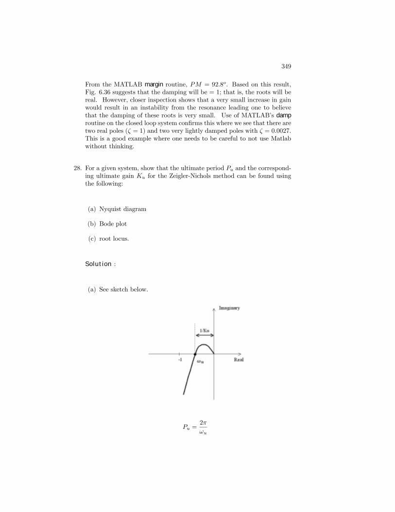
28. For a given system, show that the ultimate period Pu and the correspond-ing ultimate gain Ku for the Zeigler-Nichols method can be found usingthe following:
(a) Nyquist diagram
(b) Bode plot
(c) root locus.
Solution :
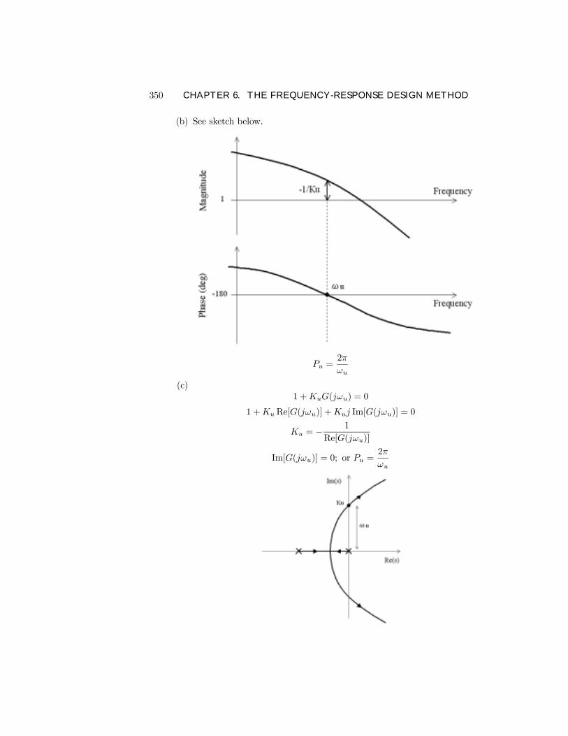
(a) See sketch below.
Pu =2π
ωu
350 CHAPTER 6. THE FREQUENCY-RESPONSE DESIGN METHOD
(b) See sketch below.
Pu =2π
ωu
(c)1 +KuG(jωu) = 0
1 +KuRe[G(jωu)] +Kuj Im[G(jωu)] = 0
Ku = − 1
Re[G(jωu)]
Im[G(jωu)] = 0; or Pu =2π
ωu
351
29. If a system has the open-loop transfer function
G(s) =ω2n
s(s+ 2ζωn)
with unity feedback, then the closed-loop transfer function is given by
T (s) =ω2n
s2 + 2ζωns+ ω2n
.
Verify the values of the PM shown in Fig. 6.36 for ζ = 0.1, 0.4, and 0.7.
Solution :
G(s) =ω2n
s(s+ 2ζωn), T (s) =
G(s)
1 +G(s)=
ω2n
s2 + 2ζωns+ ω2n
ζ PM from Eq. 6.32 PM from Fig. 6.36 PM from Bode plot0.1 10 10 11.4 (ω = 0.99 rad/sec)0.4 40 44 43.1 (ω = 0.85 rad/sec)0.7 70 65 65.2 (ω = 0.65 rad/sec)
30. Consider the unity feedback system with the open-loop transfer function
G(s) =K
s(s+ 1)[(s2/25) + 0.4(s/5) + 1].
(a) Use MATLAB to draw the Bode plots for G(jω) assuming K = 1.
(b) What gain K is required for a PM of 45? What is the GM for thisvalue of K?
(c) What is Kv when the gain K is set for PM = 45?
(d) Create a root locus with respect to K, and indicate the roots for aPM of 45.
Solution :
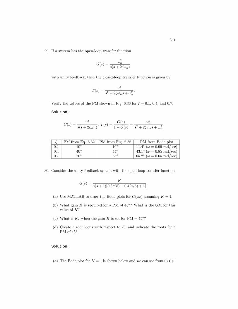
(a) The Bode plot for K = 1 is shown below and we can see from margin
352 CHAPTER 6. THE FREQUENCY-RESPONSE DESIGN METHOD
that it results in a PM = 48o.
10-2
10-1
100
101
102
10-10
10-5
100
105
Frequency (rad/sec)
Magnitude
B ode D iagram s
10-2
10-1
100
101
102
-400
-300
-200
-100
0
Frequency (rad/sec)
Phase (deg)
(b) Although diffult to read the plot above, it is clear that a very slightincrease in gain will lower the PM to 45o, so try K = 1.1. The marginroutine shows that this yields PM = 45o and GM = 15 db.
(c) Kv = lims→0sKG(s) = K = 1.1 when K is set for PM=45
Kv = 1.1
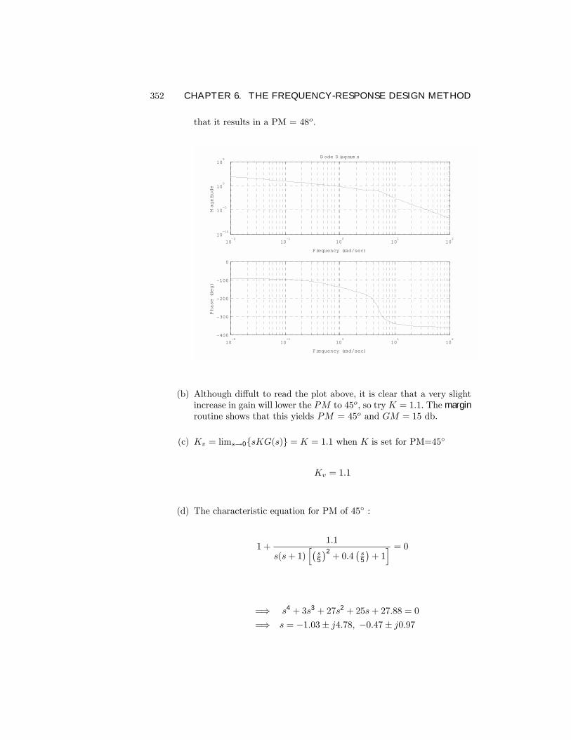
(d) The characteristic equation for PM of 45 :
1 +1.1
s(s+ 1)h¡
s5
¢2+ 0.4
¡s5
¢+ 1i = 0
=⇒ s4 + 3s3 + 27s2 + 25s+ 27.88 = 0
=⇒ s = −1.03± j4.78, −0.47± j0.97
353
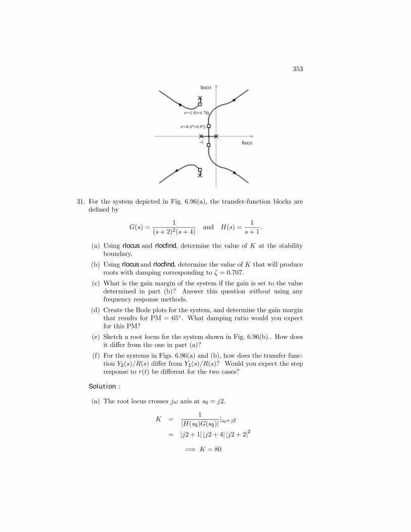
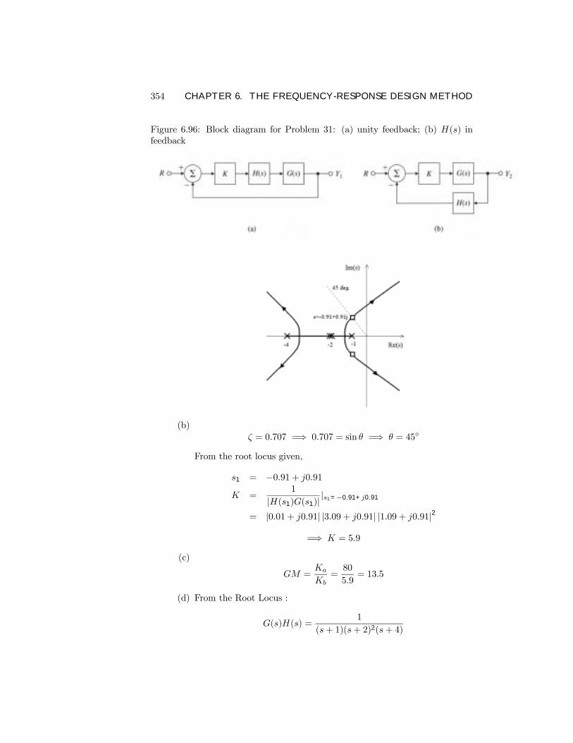
31. For the system depicted in Fig. 6.96(a), the transfer-function blocks aredeÞned by
G(s) =1
(s+ 2)2(s+ 4)and H(s) =
1
s+ 1.
(a) Using rlocus and rlocfind, determine the value of K at the stabilityboundary.
(b) Using rlocus and rlocfind, determine the value of K that will produceroots with damping corresponding to ζ = 0.707.
(c) What is the gain margin of the system if the gain is set to the valuedetermined in part (b)? Answer this question without using anyfrequency response methods.
(d) Create the Bode plots for the system, and determine the gain marginthat results for PM = 65. What damping ratio would you expectfor this PM?
(e) Sketch a root locus for the system shown in Fig. 6.96(b).. How doesit differ from the one in part (a)?
(f) For the systems in Figs. 6.96(a) and (b), how does the transfer func-tion Y2(s)/R(s) differ from Y1(s)/R(s)? Would you expect the stepresponse to r(t) be different for the two cases?
Solution :
(a) The root locus crosses jω axis at s0 = j2.
K =1
|H(s0)G(s0)| |s0=j2
= |j2 + 1| |j2 + 4| |j2 + 2|2
=⇒ K = 80
354 CHAPTER 6. THE FREQUENCY-RESPONSE DESIGN METHOD
Figure 6.96: Block diagram for Problem 31: (a) unity feedback; (b) H(s) infeedback
(b)ζ = 0.707 =⇒ 0.707 = sin θ =⇒ θ = 45
From the root locus given,
s1 = −0.91 + j0.91K =
1
|H(s1)G(s1)| |s1=−0.91+j0.91
= |0.01 + j0.91| |3.09 + j0.91| |1.09 + j0.91|2
=⇒ K = 5.9
(c)
GM =Ka
Kb=80
5.9= 13.5
(d) From the Root Locus :
G(s)H(s) =1
(s+ 1)(s+ 2)2(s+ 4)
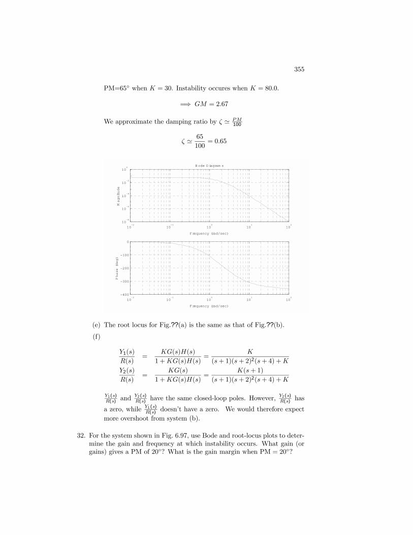
355
PM=65 when K = 30. Instability occures when K = 80.0.
=⇒ GM = 2.67
We approximate the damping ratio by ζ ' PM100
ζ ' 65
100= 0.65
10-2
10-1
100
101
102
10-8
10-6
10-4
10-2
100
Frequency (rad/sec)
Magnitude
B ode D iagram s
10-2
10-1
100
101
102
-400
-300
-200
-100
0
Frequency (rad/sec)
Phase (deg)
(e) The root locus for Fig.??(a) is the same as that of Fig.??(b).
(f)
Y1(s)
R(s)=
KG(s)H(s)
1 +KG(s)H(s)=
K
(s+ 1)(s+ 2)2(s+ 4) +K
Y2(s)
R(s)=
KG(s)
1 +KG(s)H(s)=
K(s+ 1)
(s+ 1)(s+ 2)2(s+ 4) +K
Y1(s)R(s) and
Y2(s)R(s) have the same closed-loop poles. However,
Y2(s)R(s) has
a zero, while Y1(s)R(s) doesnt have a zero. We would therefore expect
more overshoot from system (b).
32. For the system shown in Fig. 6.97, use Bode and root-locus plots to deter-mine the gain and frequency at which instability occurs. What gain (orgains) gives a PM of 20? What is the gain margin when PM = 20?
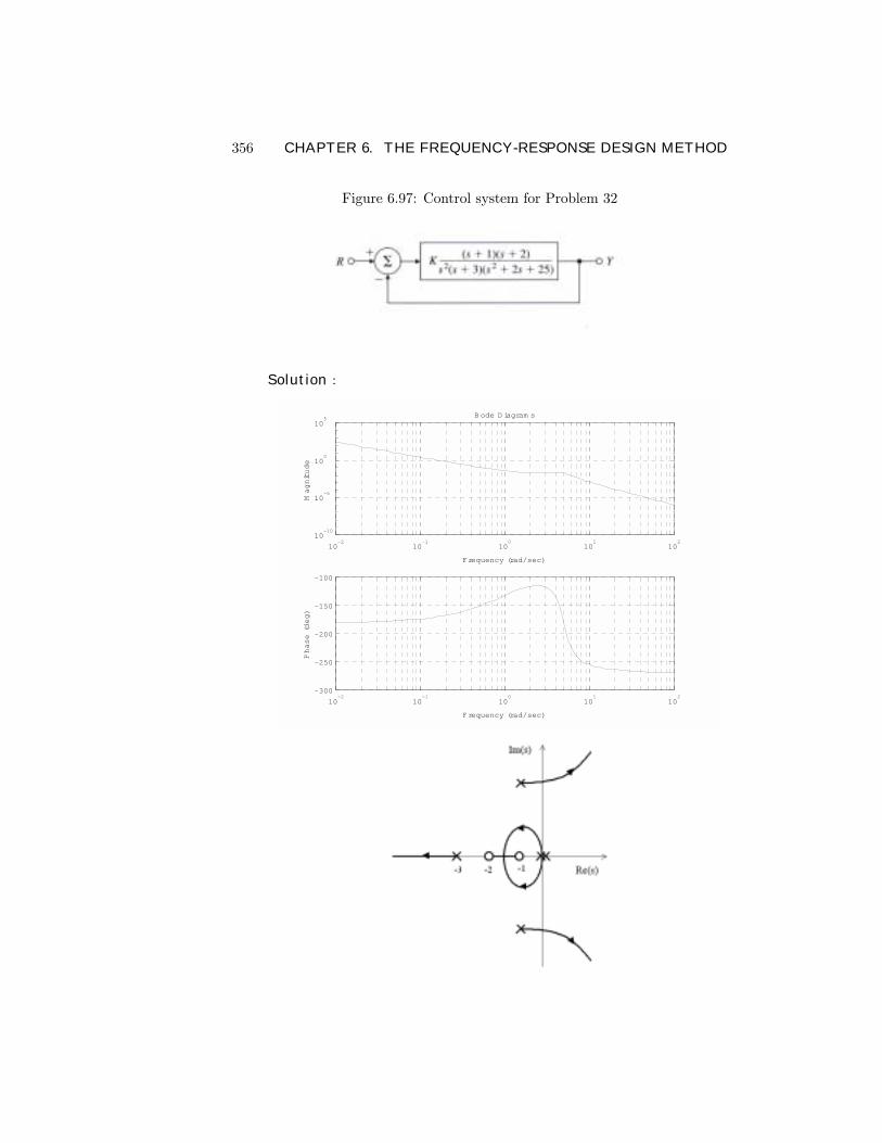
356 CHAPTER 6. THE FREQUENCY-RESPONSE DESIGN METHOD
Figure 6.97: Control system for Problem 32
Solution :
10-2
10-1
100
101
102
10-10
10-5
100
105
Frequency (rad/sec)
Magnitude
B ode D iagram s
10-2
10-1
100
101
102
-300
-250
-200
-150
-100
Frequency (rad/sec)
Phase (deg)
357
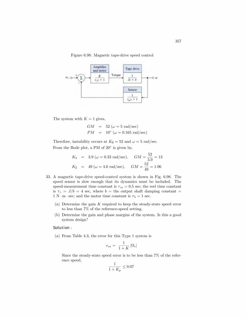
Figure 6.98: Magnetic tape-drive speed control
The system with K = 1 gives,
GM = 52 (ω = 5 rad/sec)
PM = 10 (ω = 0.165 rad/sec)
Therefore, instability occurs at K0 = 52 and ω = 5 rad/sec.
From the Bode plot, a PM of 20 is given by,
K1 = 3.9 (ω = 0.33 rad/sec), GM =52
3.9= 13
K2 = 49 (ω = 4.6 rad/sec), GM =52
49= 1.06
33. A magnetic tape-drive speed-control system is shown in Fig. 6.98. Thespeed sensor is slow enough that its dynamics must be included. Thespeed-measurement time constant is τm = 0.5 sec; the reel time constantis τr = J/b = 4 sec, where b = the output shaft damping constant =1 N ·m · sec; and the motor time constant is τ1 = 1 sec.
(a) Determine the gain K required to keep the steady-state speed errorto less than 7% of the reference-speed setting.
(b) Determine the gain and phase margins of the system. Is this a goodsystem design?
Solution :
(a) From Table 4.3, the error for this Type 1 system is
ess =1
1 +K|Ωc|
Since the steady-state speed error is to be less than 7% of the refer-ence speed,
1
1 +Kp≤ 0.07
358 CHAPTER 6. THE FREQUENCY-RESPONSE DESIGN METHOD
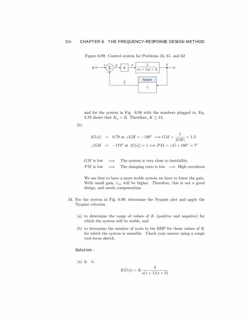
Figure 6.99: Control system for Problems 34, 61, and 62
and for the system in Fig. 6.98 with the numbers plugged in, Eq.4.70 shows that Kp = K. Therefore, K ≥ 13.
(b)
|G(s)| = 0.79 at ∠GH = −180 =⇒ GM =1
|GH| = 1.3∠GH = −173 at |G(s)| = 1 =⇒ PM = ∠G+ 180 = 7
GM is low =⇒ The system is very close to instability.
PM is low =⇒ The damping ratio is low. =⇒ High overshoot.
We see that to have a more stable system we have to lower the gain.With small gain, ess will be higher. Therefore, this is not a gooddesign, and needs compensation.
34. For the system in Fig. 6.99, determine the Nyquist plot and apply theNyquist criterion
(a) to determine the range of values of K (positive and negative) forwhich the system will be stable, and
(b) to determine the number of roots in the RHP for those values of Kfor which the system is unstable. Check your answer using a roughroot-locus sketch.
Solution :
(a) & b.
KG(s) = K3
s(s+ 1)(s+ 3)
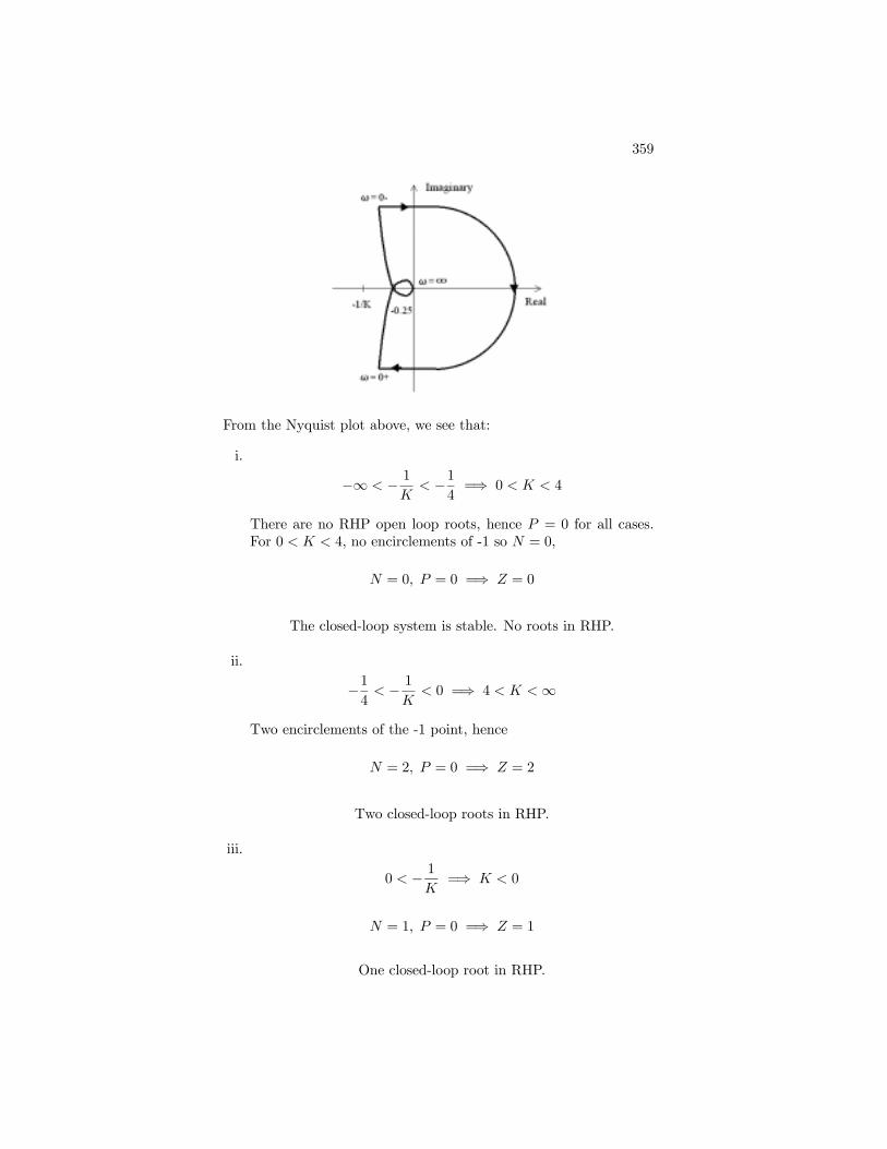
359
From the Nyquist plot above, we see that:
i.
−∞ < − 1K< −1
4=⇒ 0 < K < 4
There are no RHP open loop roots, hence P = 0 for all cases.For 0 < K < 4, no encirclements of -1 so N = 0,
N = 0, P = 0 =⇒ Z = 0
The closed-loop system is stable. No roots in RHP.
ii.
−14< − 1
K< 0 =⇒ 4 < K <∞
Two encirclements of the -1 point, hence
N = 2, P = 0 =⇒ Z = 2
Two closed-loop roots in RHP.
iii.
0 < − 1K
=⇒ K < 0
N = 1, P = 0 =⇒ Z = 1
One closed-loop root in RHP.
360 CHAPTER 6. THE FREQUENCY-RESPONSE DESIGN METHOD
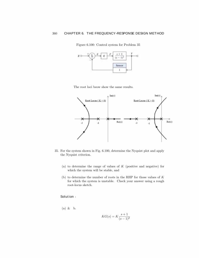
Figure 6.100: Control system for Problem 35
The root loci beow show the same results.
35. For the system shown in Fig. 6.100, determine the Nyquist plot and applythe Nyquist criterion.
(a) to determine the range of values of K (positive and negative) forwhich the system will be stable, and
(b) to determine the number of roots in the RHP for those values of Kfor which the system is unstable. Check your answer using a roughroot-locus sketch.
Solution :
(a) & b.
KG(s) = Ks+ 1
(s− 1)2
361
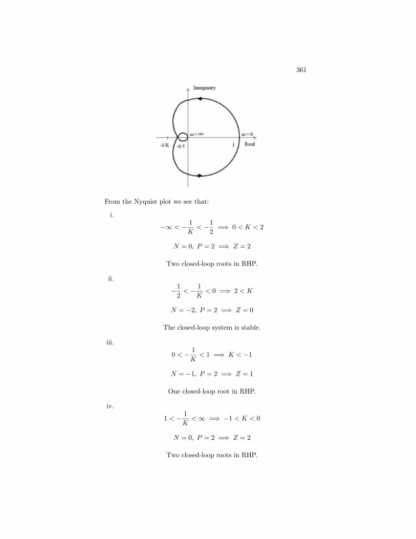
From the Nyquist plot we see that:
i.
−∞ < − 1K< −1
2=⇒ 0 < K < 2
N = 0, P = 2 =⇒ Z = 2
Two closed-loop roots in RHP.
ii.
−12< − 1
K< 0 =⇒ 2 < K
N = −2, P = 2 =⇒ Z = 0
The closed-loop system is stable.
iii.
0 < − 1K< 1 =⇒ K < −1
N = −1, P = 2 =⇒ Z = 1
One closed-loop root in RHP.
iv.
1 < − 1K<∞ =⇒ −1 < K < 0
N = 0, P = 2 =⇒ Z = 2
Two closed-loop roots in RHP.
362 CHAPTER 6. THE FREQUENCY-RESPONSE DESIGN METHOD
Figure 6.101: Control system for Problem 36
These results are conÞrmed by looking at the root loci below:
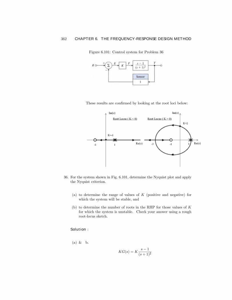
36. For the system shown in Fig. 6.101, determine the Nyquist plot and applythe Nyquist criterion.
(a) to determine the range of values of K (positive and negative) forwhich the system will be stable, and
(b) to determine the number of roots in the RHP for those values of Kfor which the system is unstable. Check your answer using a roughroot-locus sketch.
Solution :
(a) & b.
KG(s) = Ks− 1(s+ 1)2
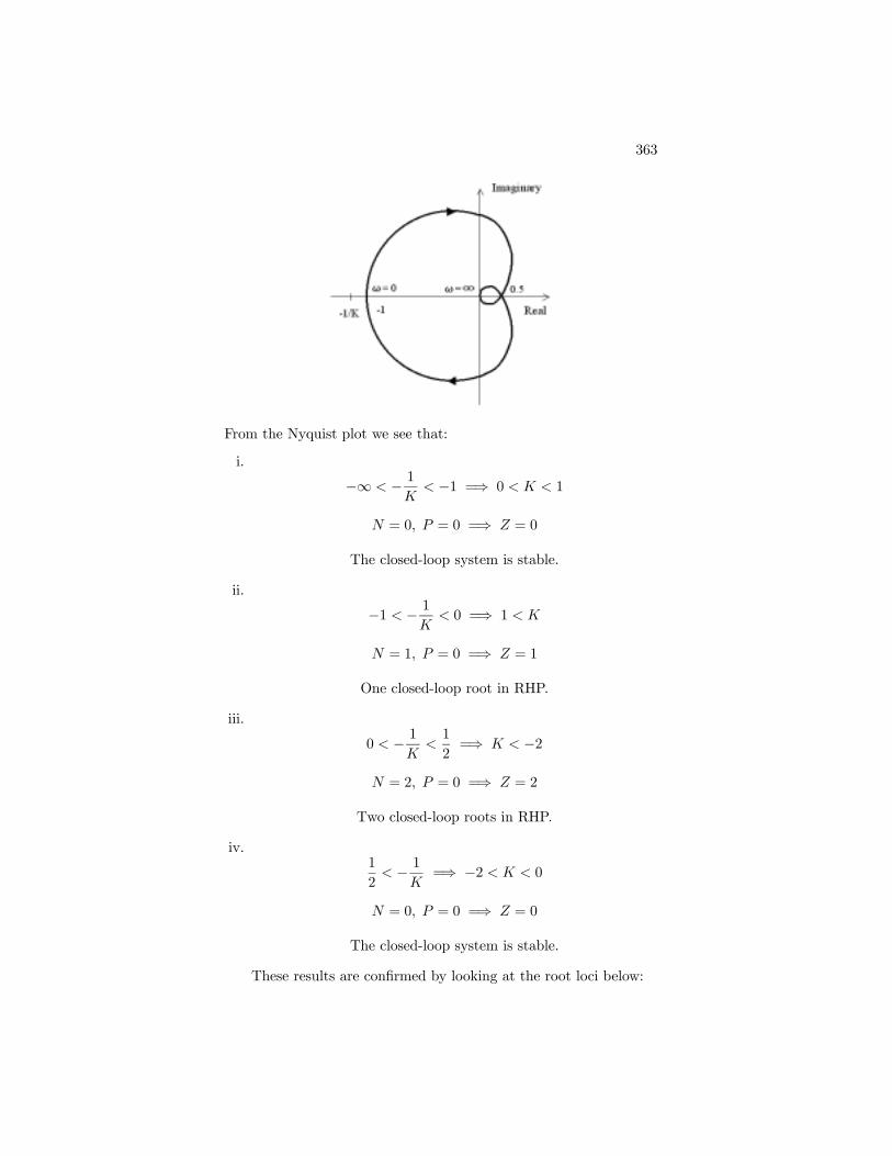
363
From the Nyquist plot we see that:
i.
−∞ < − 1K< −1 =⇒ 0 < K < 1
N = 0, P = 0 =⇒ Z = 0
The closed-loop system is stable.
ii.
−1 < − 1K< 0 =⇒ 1 < K
N = 1, P = 0 =⇒ Z = 1
One closed-loop root in RHP.
iii.
0 < − 1K<1
2=⇒ K < −2
N = 2, P = 0 =⇒ Z = 2
Two closed-loop roots in RHP.
iv.1
2< − 1
K=⇒ −2 < K < 0
N = 0, P = 0 =⇒ Z = 0
The closed-loop system is stable.
These results are conÞrmed by looking at the root loci below:
364 CHAPTER 6. THE FREQUENCY-RESPONSE DESIGN METHOD
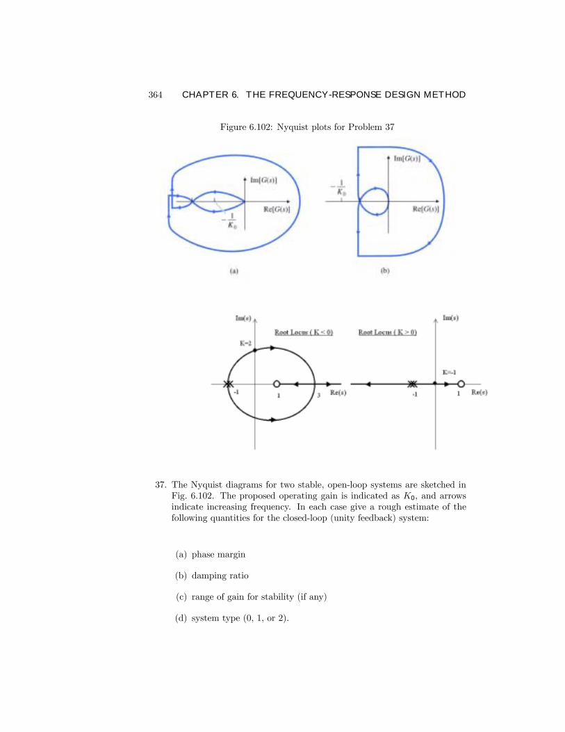
Figure 6.102: Nyquist plots for Problem 37
37. The Nyquist diagrams for two stable, open-loop systems are sketched inFig. 6.102. The proposed operating gain is indicated as K0, and arrowsindicate increasing frequency. In each case give a rough estimate of thefollowing quantities for the closed-loop (unity feedback) system:
(a) phase margin
(b) damping ratio
(c) range of gain for stability (if any)
(d) system type (0, 1, or 2).

365
Solution :
For both, with K = K0:
N = 0, P = 0 =⇒ Z = 0
Therefore, the closed-loop system is stable.
Fig.6.102(a) Fig.6.102(b)a. PM '17 '45b. Damping ratio 0.17(' 17
100) 0.45(' 45100)
c. To determine the range of gain for stability, call the value of K wherethe plots cross the negative real axis as K1. For case (a), K > K1 forstability because gains lower than this amount will cause the -1 point tobe encircled. For case (b), K < K1 for stability because gains greaterthan this amount will cause the -1 point to be encircled.
d. For case (a), the 360o loop indicates two poles at the origin, hence thesystem is Type 2. For case (b), the 180o loop indicates one pole at theorigin, hence the system is Type 1.
38. The steering dynamics of a ship are represented by the transfer function
V (s)
δr(s)= G(s) =
K[−(s/0.142) + 1]s(s/0.325 + 1)(s/0.0362) + 1)
,
where v is the ships lateral velocity in meters per second, and δr is therudder angle in radians.
(a) Use the MATLAB command bode to plot the log magnitude andphase of G(jω) for K = 0.2
(b) On your plot, indicate the crossover frequency, PM, and GM,
(c) Is the ship steering system stable with K = 0.2?
366 CHAPTER 6. THE FREQUENCY-RESPONSE DESIGN METHOD
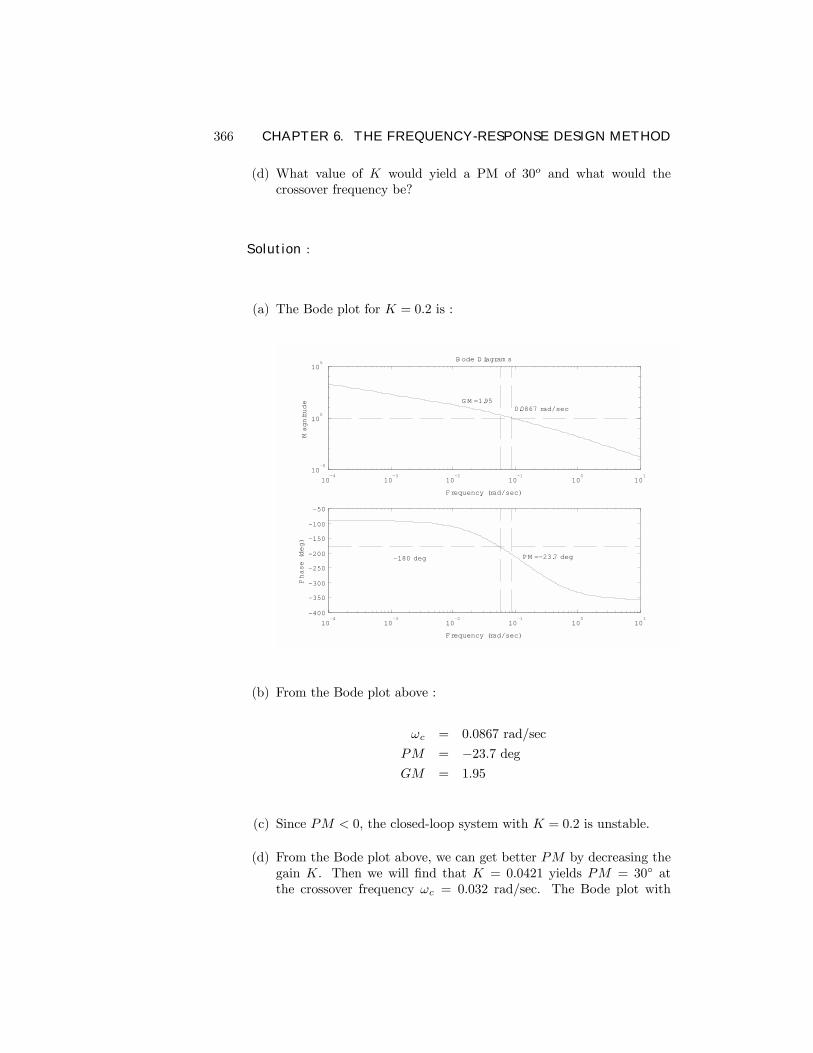
(d) What value of K would yield a PM of 30o and what would thecrossover frequency be?
Solution :
(a) The Bode plot for K = 0.2 is :
10-4
10-3
10-2
10-1
100
101
10-5
100
105
Frequency (rad/sec)
Magnitude
B ode D iagram s
0.0867 rad/secG M =1.95
10-4
10-3
10-2
10-1
100
101
-400
-350
-300
-250
-200
-150
-100
-50
Frequency (rad/sec)
Phase (deg)
-180 deg PM =-23.7 deg
(b) From the Bode plot above :
ωc = 0.0867 rad/sec
PM = −23.7 degGM = 1.95
(c) Since PM < 0, the closed-loop system with K = 0.2 is unstable.
(d) From the Bode plot above, we can get better PM by decreasing thegain K. Then we will Þnd that K = 0.0421 yields PM = 30 atthe crossover frequency ωc = 0.032 rad/sec. The Bode plot with
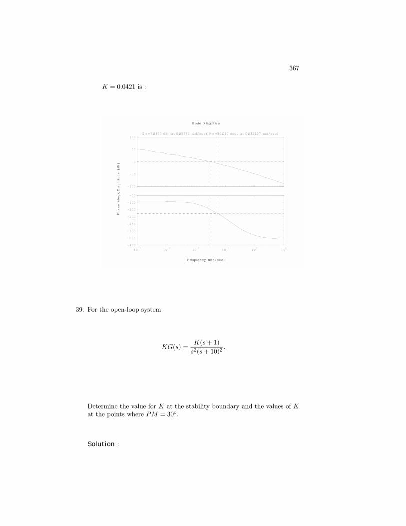
367
K = 0.0421 is :
Frequency (rad/sec)
Phase (deg); M
agnitude (dB)
B ode D iagram s
-100
-50
0
50
100G m =7.6803 dB (at 0.05762 rad/sec), Pm =30.017 deg. (at 0.032127 rad/sec)
10-4
10-3
10-2
10-1
100
101
-400
-350
-300
-250
-200
-150
-100
-50
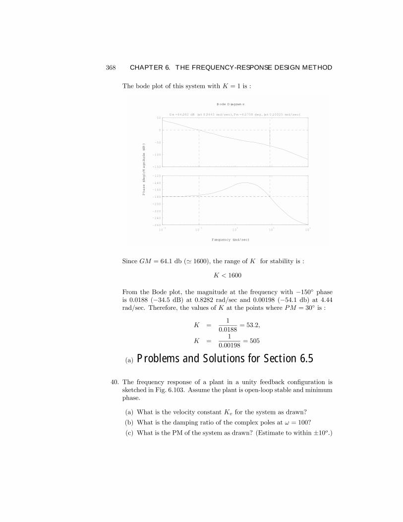
39. For the open-loop system
KG(s) =K(s+ 1)
s2(s+ 10)2.
Determine the value for K at the stability boundary and the values of Kat the points where PM = 30.
Solution :
368 CHAPTER 6. THE FREQUENCY-RESPONSE DESIGN METHOD
The bode plot of this system with K = 1 is :
Frequency (rad/sec)
Phase (deg); M
agnitude (dB)
B ode D iagram s
-150
-100
-50
0
50G m =64.082 dB (at 8.9443 rad/sec), Pm =4.5758 deg. (at 0.10025 rad/sec)
10-2
10-1
100
101
102
-260
-240
-220
-200
-180
-160
-140
-120
Since GM = 64.1 db (' 1600), the range of K for stability is :
K < 1600
From the Bode plot, the magnitude at the frequency with −150 phaseis 0.0188 (−34.5 dB) at 0.8282 rad/sec and 0.00198 (−54.1 db) at 4.44rad/sec. Therefore, the values of K at the points where PM = 30 is :
K =1
0.0188= 53.2,
K =1
0.00198= 505
(a) Problems and Solutions for Section 6.5
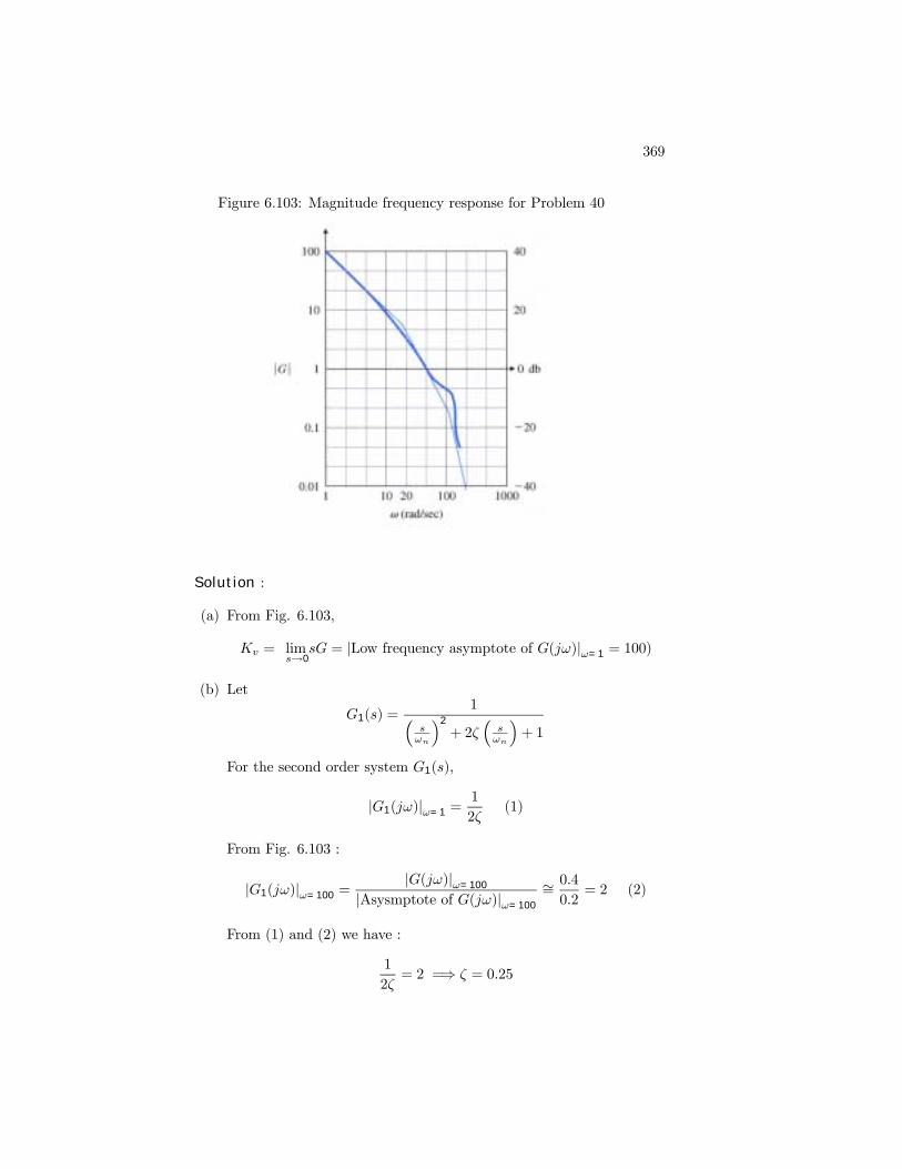
40. The frequency response of a plant in a unity feedback conÞguration issketched in Fig. 6.103. Assume the plant is open-loop stable and minimumphase.
(a) What is the velocity constant Kv for the system as drawn?
(b) What is the damping ratio of the complex poles at ω = 100?
(c) What is the PM of the system as drawn? (Estimate to within ±10o.)
369
Figure 6.103: Magnitude frequency response for Problem 40
Solution :
(a) From Fig. 6.103,
Kv = lims→0
sG = |Low frequency asymptote of G(jω)|ω=1 = 100)
(b) Let
G1(s) =1³
sωn
´2
+ 2ζ³sωn
´+ 1
For the second order system G1(s),
|G1(jω)|ω=1 =1
2ζ(1)
From Fig. 6.103 :
|G1(jω)|ω=100 =|G(jω)|ω=100
|Asysmptote of G(jω)|ω=100
∼= 0.4
0.2= 2 (2)
From (1) and (2) we have :
1
2ζ= 2 =⇒ ζ = 0.25
370 CHAPTER 6. THE FREQUENCY-RESPONSE DESIGN METHOD
(c) Since the plant is a minimum phase system, we can apply the Bodesapproximate gain-phase relationship.
When |G| = 1, the slope of |G| curve is ∼= -2.=⇒ ∠G(jω) ∼= −2× 90 = −180
PM ∼= ∠G(jω) + 180 = 0
Note : Actual PM by Matlab calculation is 6.4, so this approxima-tion is within the desired accuracy.
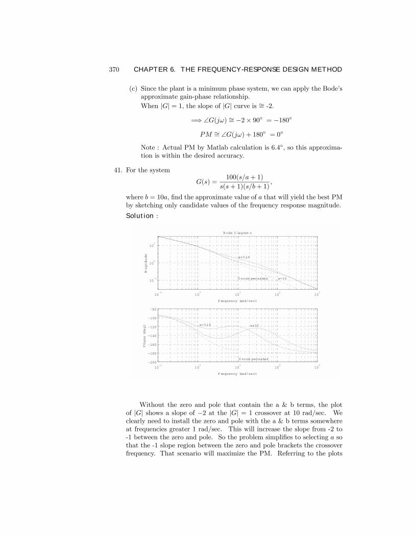
41. For the system
G(s) =100(s/a+ 1)
s(s+ 1)(s/b+ 1),
where b = 10a, Þnd the approximate value of a that will yield the best PMby sketching only candidate values of the frequency response magnitude.
Solution :
10-1
100
101
102
103
10-2
100
102
Frequency (rad/sec)
Magnitude
B ode D iagram s
a=3.16
a=10U ncom pensated
10-1
100
101
102
103
-200
-180
-160
-140
-120
-100
-80
Frequency (rad/sec)
Phase (deg) a=3.16 a=10
U ncom pensated
Without the zero and pole that contain the a & b terms, the plotof |G| shows a slope of −2 at the |G| = 1 crossover at 10 rad/sec. Weclearly need to install the zero and pole with the a & b terms somewhereat frequencies greater 1 rad/sec. This will increase the slope from -2 to-1 between the zero and pole. So the problem simpliÞes to selecting a sothat the -1 slope region between the zero and pole brackets the crossoverfrequency. That scenario will maximize the PM. Referring to the plots
371
above, we see that 3.16 < a < 10, makes the slope of the asymptote of |G|be −1 at the crossover and represent the two extremes of possibilities for a-1 slope. The maximum PM will occur half way between these extremeson a log scale, or
=⇒ a =√3.16× 10 = 5.6
Note : Actual PM is as follows :
PM = 46.8 for a = 3.16 (ωc = 25.0 rad/sec)PM = 58.1 for a = 5.6 (ωc = 17.8 rad/sec)PM = 49.0 for a = 10 (ωc = 12.6 rad/sec)
Problem and Solution for Section 6.6
42. For the open-loop system
KG(s) =K(s+ 1)
s2(s+ 10)2.
Determine the value for K that will yield PM ≥ 30 and the maximumpossible closed-loop bandwidth. Use MATLAB to Þnd the bandwidth.
Solution :
From the result of Problem 6.39., the value of K that will yield PM ≥ 30is :
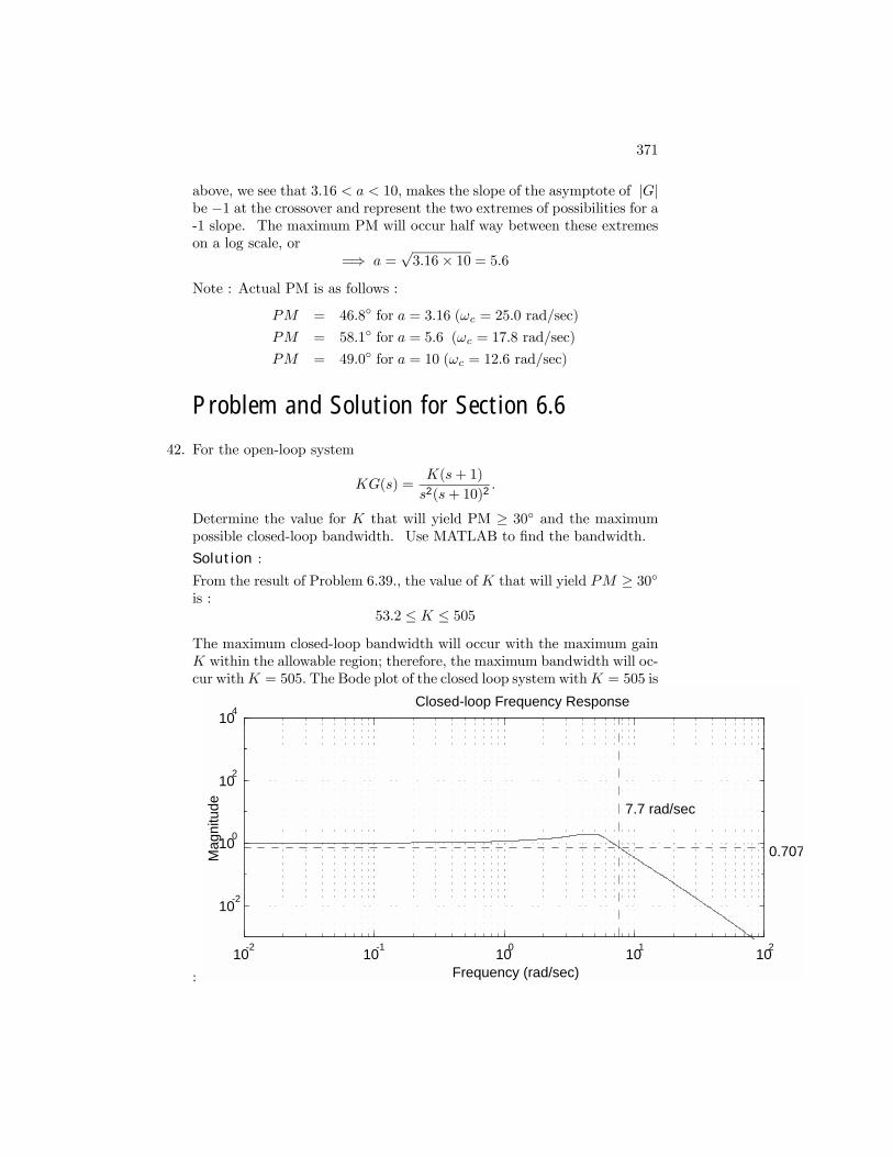
53.2 ≤ K ≤ 505The maximum closed-loop bandwidth will occur with the maximum gainK within the allowable region; therefore, the maximum bandwidth will oc-cur withK = 505. The Bode plot of the closed loop system withK = 505 is
:
10-2 10-1 100 101 102
10-2
100
102
104
Frequency (rad/sec)
Mag
nitu
de
Closed-loop Frequency Response
0.707
7.7 rad/sec
372 CHAPTER 6. THE FREQUENCY-RESPONSE DESIGN METHOD
Looking at the point with Magnitude 0.707(-3 db), the maximum possibleclosed-loop bandwidth is :
ωBW, max ' 7.7 rad/sec.
Problems and Solutions for Section 6.743. For the lead compensator
D(s) =Ts+ 1
αTs+ 1,
where α < 1.
(a) Show that the phase of the lead compensator is given by
φ = tan−1(Tω)− tan−1(αTω).
(b) Show that the frequency where the phase is maximum is given by
ωmax =1
T√α,
and that the maximum phase corresponds to
sinφmax =1− α1 + α
.
(c) Rewrite your expression for ωmax to show that the maximum-phasefrequency occurs at the geometric mean of the two corner frequencieson a logarithmic scale:
logωmax =1
2
µlog
1
T+ log
1
αT
¶.
(d) To derive the same results in terms of the pole-zero locations, rewriteD(s) as
D(s) =s+ z
s+ p,
and then show that the phase is given by
φ = tan−1
µω
|z|¶− tan−1
µω
|p|¶,
such thatωmax =
p|z||p|.
Hence the frequency at which the phase is maximum is the squareroot of the product of the pole and zero locations.
373
Solution :
(a) The frequency response is obtained by letting s = jω,
D(jω) = KTjω + 1
αTjω + 1
The phase is given by,φ = tan−1(Tω)− tan−1(αTω)
(b) Using the trigonometric relationship,
tan(A−B) = tan(A)− tan(B)1 + tan(A) tan(B)
then
tan(φ) =Tω − αTω1− αT 2ω2
and since,
sin2(φ) =tan2(φ)
1 + tan2(φ)
then
sin(φ) =
sω2T 2(1− α)2
1 + α2ω4T 4 + (1 + α2)ω2T 2
To determine the frequency at which the phase is a maximum, let usset the derivative with respect to ω equal to zero,
d sin(φ)
dω= 0
which leads to2ωT 2(1− α)2(1− αω4T 4) = 0
The value ω = 0 gives the maximum of the function and setting thesecond part of the above equation to zero then,
ω4 =1
α2T 4
or
ωmax =1√αT
The maximum phase contribution, that is, the peak of the ∠D(s)curve corresponds to,
sinφmax =1− α1 + α
or
α =1− sinφmax
1 + sinφmax
tanφmax =ωmaxT − αωmaxT
1 + ω2maxT
2=1− α2√α
374 CHAPTER 6. THE FREQUENCY-RESPONSE DESIGN METHOD
(c) The maxmum frequency occurs midway between the two break fre-quencies on a logarithmic scale,
logωmax = log
1√T√αT
= log1√T+ log
1√αT
=1
2
µlog
1
T+ log
1
αT
¶as shown in Fig. 6.52.
(d) Alternatively, we may state these results in terms of the pole-zerolocations. Rewrite D(s) as,
D(s) = K(s+ z)
(s+ p)
then
D(jω) = K(jω + z)
(jω + p)
and
φ = tan−1
µω
|z|¶− tan−1
µω
|p|
or
tanφ =
ω|z| − ω
|p|1 + ω
|z|ω|p|
Setting the derivative of the above equation to zero we Þnd,µω
|z| −ω
|p|¶µ
1 +ω2
|z| |p|¶− 2ω
|z| |p|µω
|z| −ω
|p|¶= 0
and
ωmax =p|z| |p|
and
logωmax =1
2(log |z|+ log |p|)
Hence the frequency at which the phase is maximum is the squareroot of the product of the pole and zero locations.
44. For the third-order servo system
G(s) =50, 000
s(s+ 10)(s+ 50).
375
Design a lead compensator so that PM ≥50 and ωBW ≥ 20 rad/sec usingBode plot sketches, then verify and reÞne your design using MATLAB.
Solution :
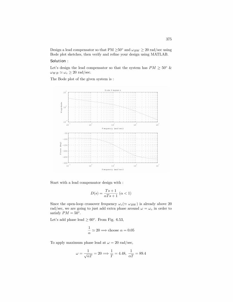
Lets design the lead compensator so that the system has PM ≥ 50 &ωWB ' ωc ≥ 20 rad/sec.The Bode plot of the given system is :
10-1
100
101
102
103
10-5
100
105
Frequency (rad/sec)
Magnitude
B ode D iagram s
10-1
100
101
102
103
-300
-250
-200
-150
-100
-50
Frequency (rad/sec)
Phase (deg)
Start with a lead compensator design with :
D(s) =Ts+ 1
αTs+ 1(α < 1)
Since the open-loop crossover frequency ωc(' ωBW ) is already above 20rad/sec, we are going to just add extra phase around ω = ωc in order tosatisfy PM = 50.
Lets add phase lead ≥ 60. From Fig. 6.53,
1
α' 20 =⇒ choose α = 0.05
To apply maximum phase lead at ω = 20 rad/sec,
ω =1√αT
= 20 =⇒ 1
T= 4.48,
1
αT= 89.4
376 CHAPTER 6. THE FREQUENCY-RESPONSE DESIGN METHOD
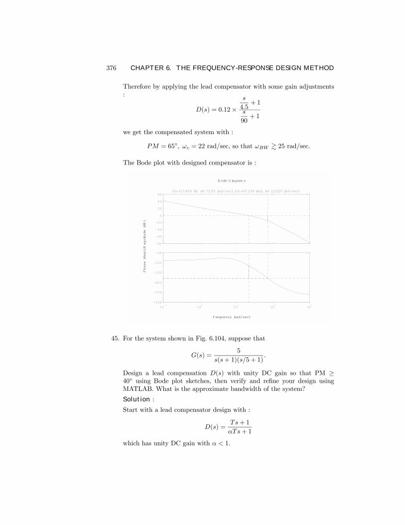
Therefore by applying the lead compensator with some gain adjustments:
D(s) = 0.12×s
4.5+ 1
s
90+ 1
we get the compensated system with :
PM = 65, ωc = 22 rad/sec, so that ωBW & 25 rad/sec.
The Bode plot with designed compensator is :
Frequency (rad/sec)
Phase (deg); M
agnitude (dB)
B ode D iagram s
-80
-60
-40
-20
0
20
40
60G m =15.854 dB (at 72.55 rad/sec), Pm =65.338 deg. (at 22.029 rad/sec)
10-1
100
101
102
103
-300
-250
-200
-150
-100
-50
45. For the system shown in Fig. 6.104, suppose that
G(s) =5
s(s+ 1)(s/5 + 1).
Design a lead compensation D(s) with unity DC gain so that PM ≥40 using Bode plot sketches, then verify and reÞne your design usingMATLAB. What is the approximate bandwidth of the system?
Solution :
Start with a lead compensator design with :
D(s) =Ts+ 1
αTs+ 1
which has unity DC gain with α < 1.
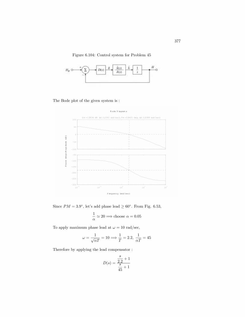
377
Figure 6.104: Control system for Problem 45
The Bode plot of the given system is :
Frequency (rad/sec)
Phase (deg); M
agnitude (dB)
B ode D iagram s
-100
-50
0
50
100G m =1.5836 dB (at 2.2361 rad/sec), Pm =3.9431 deg. (at 2.0388 rad/sec)
10-2
10-1
100
101
102
-300
-250
-200
-150
-100
-50
Since PM = 3.9, lets add phase lead ≥ 60. From Fig. 6.53,
1
α' 20 =⇒ choose α = 0.05
To apply maximum phase lead at ω = 10 rad/sec,
ω =1√αT
= 10 =⇒ 1
T= 2.2,
1
αT= 45
Therefore by applying the lead compensator :
D(s) =
s
2.2+ 1
s
45+ 1
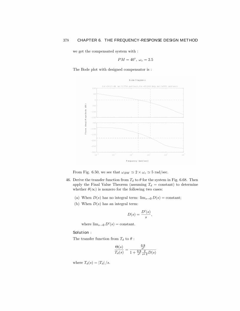
378 CHAPTER 6. THE FREQUENCY-RESPONSE DESIGN METHOD
we get the compensated system with :
PM = 40, ωc = 2.5
The Bode plot with designed compensator is :
Frequency (rad/sec)
Phase (deg); M
agnitude (dB)
B ode D iagram s
-150
-100
-50
0
50
100G m =24.13 dB (at 12.756 rad/sec), Pm =40.244 deg. (at 2.4901 rad/sec)
10-2
10-1
100
101
102
103
-300
-250
-200
-150
-100
-50
From Fig. 6.50, we see that ωBW ' 2× ωc ' 5 rad/sec.46. Derive the transfer function from Td to θ for the system in Fig. 6.68. Then
apply the Final Value Theorem (assuming Td = constant) to determinewhether θ(∞) is nonzero for the following two cases:(a) When D(s) has no integral term: lims→0D(s) = constant;
(b) When D(s) has an integral term:
D(s) =D0(s)s
,
where lims→0D0(s) = constant.
Solution :
The transfer function from Td to θ :
Θ(s)
Td(s)=
0.9s2
1 + 0.9s2
2s+2D(s)
where Td(s) = |Td| /s.
379
(a) Using the Þnal value theorem :
θ(∞) = limt→∞θ(t) = lim
s→0sΘ(t) = lim
s→0
0.9s2
s2(s+2)+1.8D(s)s2(s+2)
|Td|s
=|Td|
lims→0
D(s)=
|Td|constant
6= 0
Therefore, there will be a steady state error in θ for a constant Tdinput if there is no integral term in D(s).
(b)
θ(∞) = limt→∞θ(t) = lim
s→0sΘ(t) = lim
s→0
0.9s2
s3(s+2)+1.8D0(s)s3(s+2)
|Td|s
=0
1.8lims→0
D0(s)= 0
So when D(s) contains an integral term, a constant Td input willresult in a zero steady state error in θ.
47. The inverted pendulum has a transfer function given by Eq. (2.35), whichis similiar to
G(s) =1
s2 − 1 .
(a) Design a lead compensator to achieve a PM of 30 using Bode plotsketches, then verify and reÞne your design using MATLAB.
(b) Sketch a root locus and correlate it with the Bode plot of the system.
(c) Could you obtain the frequency response of this system experimen-tally?
Solution :
(a) Design the lead compensator :
D(s) = KTs+ 1
αTs+ 1
such that the compensated system has PM ' 30 & ωc ' 1 rad/sec.(Actually, the bandwidth or speed of response was not speciÞed, soany crossover frequency would satisfy the problem statement.)
α =1− sin(30)1 + sin(30)
= 0.32
To apply maximum phase lead at ω = 1 rad/sec,
ω =1√αT
= 1 =⇒ 1
T= 0.57,
1
αT= 1.77
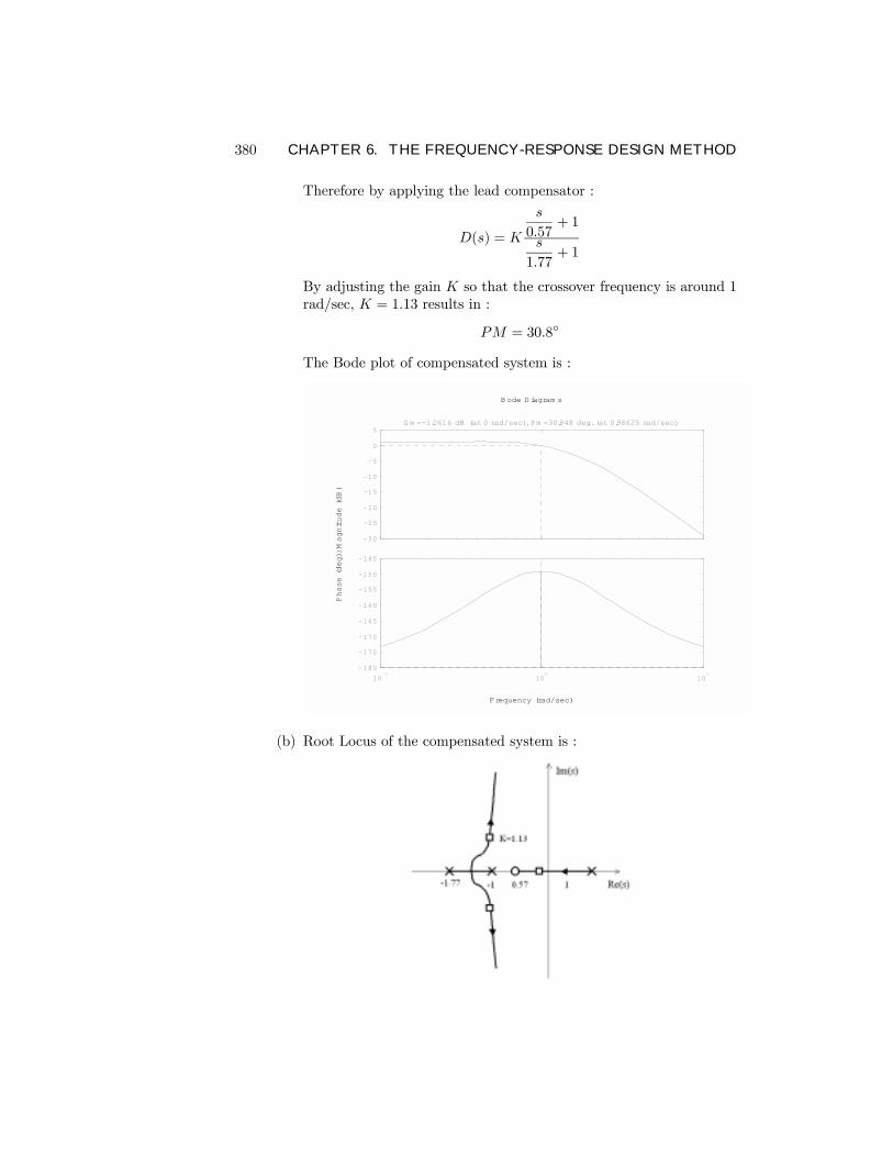
380 CHAPTER 6. THE FREQUENCY-RESPONSE DESIGN METHOD
Therefore by applying the lead compensator :
D(s) = K
s
0.57+ 1
s
1.77+ 1
By adjusting the gain K so that the crossover frequency is around 1rad/sec, K = 1.13 results in :
PM = 30.8
The Bode plot of compensated system is :
Frequency (rad/sec)
Phase (deg); M
agnitude (dB)
B ode D iagram s
-30
-25
-20
-15
-10
-5
0
5G m =-1.0616 dB (at 0 rad/sec), Pm =30.848 deg. (at 0.98625 rad/sec)
10-1
100
101
-180
-175
-170
-165
-160
-155
-150
-145
(b) Root Locus of the compensated system is :
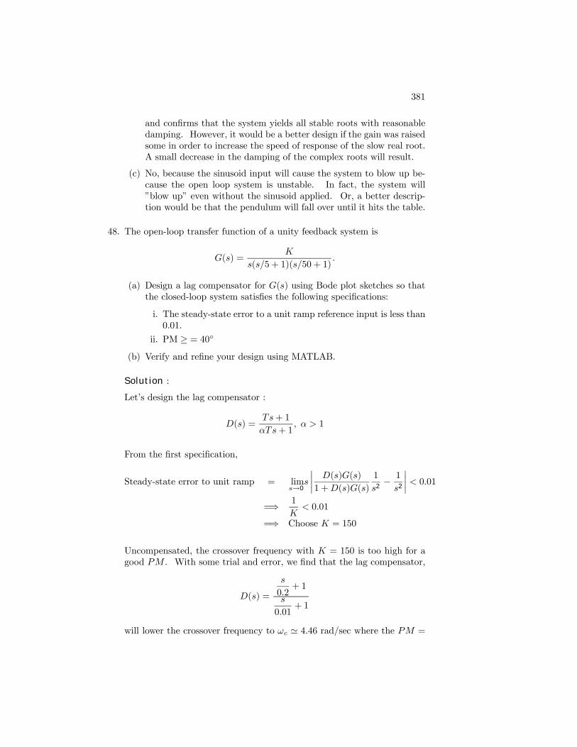
381
and conÞrms that the system yields all stable roots with reasonabledamping. However, it would be a better design if the gain was raisedsome in order to increase the speed of response of the slow real root.A small decrease in the damping of the complex roots will result.
(c) No, because the sinusoid input will cause the system to blow up be-cause the open loop system is unstable. In fact, the system willblow up even without the sinusoid applied. Or, a better descrip-tion would be that the pendulum will fall over until it hits the table.
48. The open-loop transfer function of a unity feedback system is
G(s) =K
s(s/5 + 1)(s/50 + 1).
(a) Design a lag compensator for G(s) using Bode plot sketches so thatthe closed-loop system satisÞes the following speciÞcations:
i. The steady-state error to a unit ramp reference input is less than0.01.
ii. PM ≥ = 40
(b) Verify and reÞne your design using MATLAB.
Solution :
Lets design the lag compensator :
D(s) =Ts+ 1
αTs+ 1, α > 1
From the Þrst speciÞcation,
Steady-state error to unit ramp = lims→0
s
¯D(s)G(s)
1 +D(s)G(s)
1
s2− 1
s2
¯< 0.01
=⇒ 1
K< 0.01
=⇒ Choose K = 150
Uncompensated, the crossover frequency with K = 150 is too high for agood PM . With some trial and error, we Þnd that the lag compensator,
D(s) =
s
0.2+ 1
s
0.01+ 1
will lower the crossover frequency to ωc ' 4.46 rad/sec where the PM =
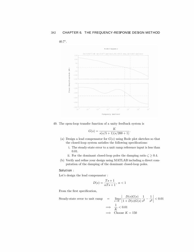
382 CHAPTER 6. THE FREQUENCY-RESPONSE DESIGN METHOD
40.7.
Frequency (rad/sec)
Phase (deg); M
agnitude (dB)
B ode D iagram s
-150
-100
-50
0
50
100
150G m =18.873 dB (at 15.477 rad/sec), Pm =40.71 deg. (at 4.463 rad/sec)
10-4
10-3
10-2
10-1
100
101
102
103
-300
-250
-200
-150
-100
-50
49. The open-loop transfer function of a unity feedback system is
G(s) =K
s(s/5 + 1)(s/200 + 1).
(a) Design a lead compensator for G(s) using Bode plot sketches so thatthe closed-loop system satisÞes the following speciÞcations:
i. The steady-state error to a unit ramp reference input is less than0.01.
ii. For the dominant closed-loop poles the damping ratio ζ ≥ 0.4.(b) Verify and reÞne your design using MATLAB including a direct com-
putation of the damping of the dominant closed-loop poles.
Solution :
Lets design the lead compensator :
D(s) =Ts+ 1
αTs+ 1, α < 1
From the Þrst speciÞcation,
Steady-state error to unit ramp = lims→0
s
¯D(s)G(s)
1 +D(s)G(s)
1
s2− 1
s2
¯< 0.01
=⇒ 1
K< 0.01
=⇒ Choose K = 150
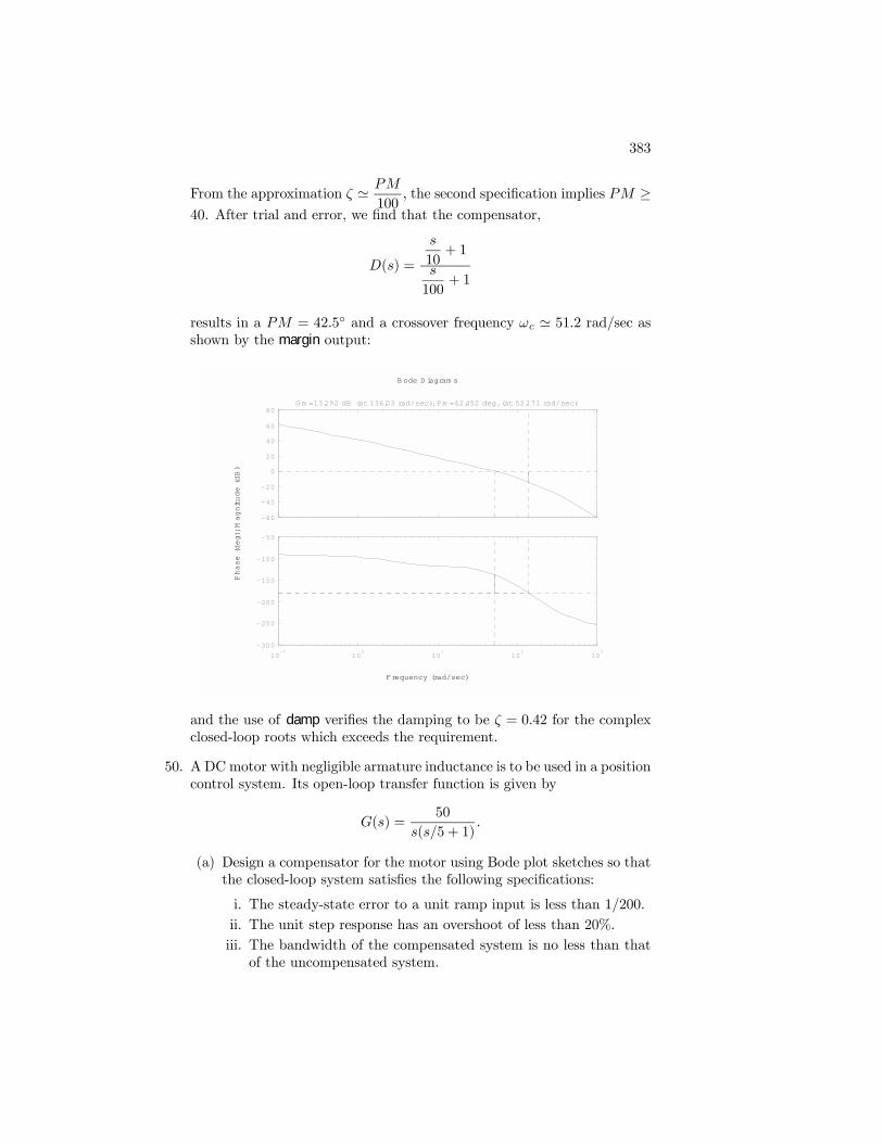
383
From the approximation ζ ' PM
100, the second speciÞcation implies PM ≥
40. After trial and error, we Þnd that the compensator,
D(s) =
s
10+ 1
s
100+ 1
results in a PM = 42.5 and a crossover frequency ωc ' 51.2 rad/sec asshown by the margin output:
Frequency (rad/sec)
Phase (deg); M
agnitude (dB)
B ode D iagram s
-60
-40
-20
0
20
40
60
80G m =13.292 dB (at 136.03 rad/sec), Pm =42.452 deg. (at 52.171 rad/sec)
10-1
100
101
102
103
-300
-250
-200
-150
-100
-50
and the use of damp veriÞes the damping to be ζ = 0.42 for the complexclosed-loop roots which exceeds the requirement.
50. A DC motor with negligible armature inductance is to be used in a positioncontrol system. Its open-loop transfer function is given by
G(s) =50
s(s/5 + 1).
(a) Design a compensator for the motor using Bode plot sketches so thatthe closed-loop system satisÞes the following speciÞcations:
i. The steady-state error to a unit ramp input is less than 1/200.
ii. The unit step response has an overshoot of less than 20%.
iii. The bandwidth of the compensated system is no less than thatof the uncompensated system.
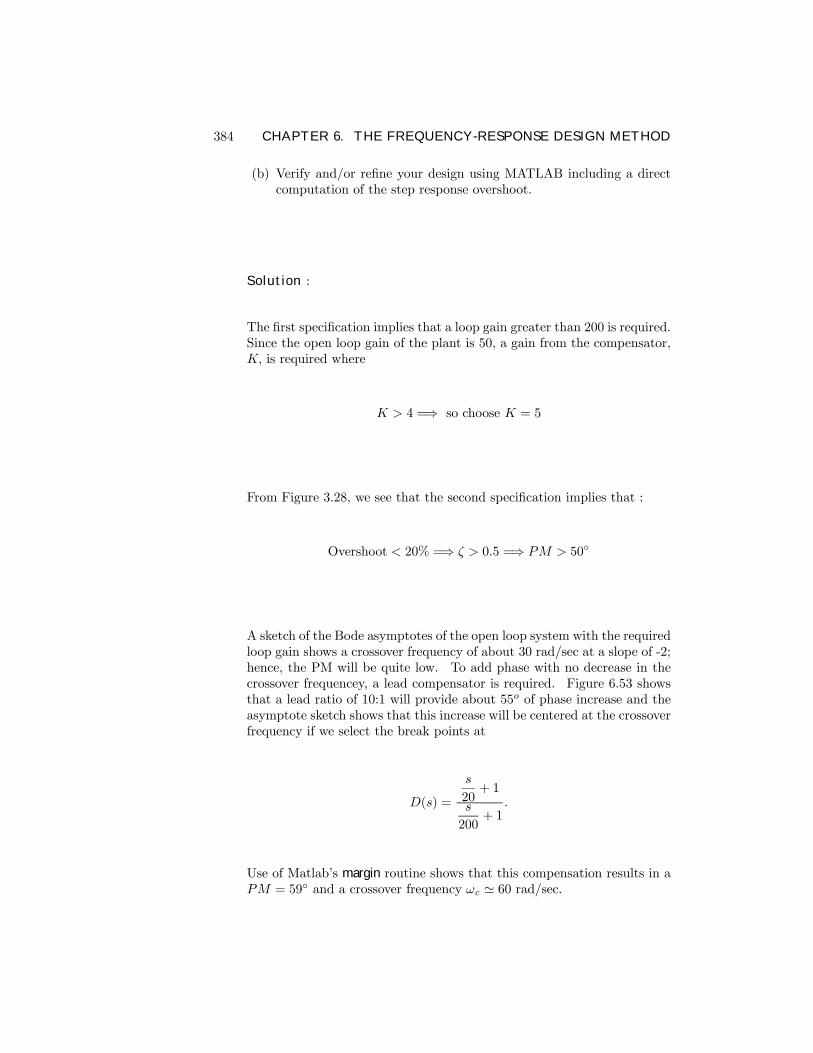
384 CHAPTER 6. THE FREQUENCY-RESPONSE DESIGN METHOD
(b) Verify and/or reÞne your design using MATLAB including a directcomputation of the step response overshoot.
Solution :
The Þrst speciÞcation implies that a loop gain greater than 200 is required.Since the open loop gain of the plant is 50, a gain from the compensator,K, is required where
K > 4 =⇒ so choose K = 5
From Figure 3.28, we see that the second speciÞcation implies that :
Overshoot < 20% =⇒ ζ > 0.5 =⇒ PM > 50
A sketch of the Bode asymptotes of the open loop system with the requiredloop gain shows a crossover frequency of about 30 rad/sec at a slope of -2;hence, the PM will be quite low. To add phase with no decrease in thecrossover frequencey, a lead compensator is required. Figure 6.53 showsthat a lead ratio of 10:1 will provide about 55o of phase increase and theasymptote sketch shows that this increase will be centered at the crossoverfrequency if we select the break points at
D(s) =
s
20+ 1
s
200+ 1
.
Use of Matlabs margin routine shows that this compensation results in aPM = 59 and a crossover frequency ωc ' 60 rad/sec.
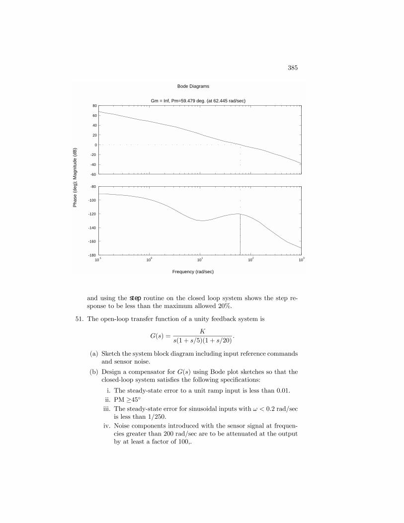
385
Frequency (rad/sec)
Phas
e (d
eg);
Mag
nitu
de (d
B)
Bode Diagrams
-60
-40
-20
0
20
40
60
80Gm = Inf, Pm=59.479 deg. (at 62.445 rad/sec)
10-1 100 101 102 103-180
-160
-140
-120
-100
-80
and using the step routine on the closed loop system shows the step re-sponse to be less than the maximum allowed 20%.
51. The open-loop transfer function of a unity feedback system is
G(s) =K
s(1 + s/5)(1 + s/20).
(a) Sketch the system block diagram including input reference commandsand sensor noise.
(b) Design a compensator for G(s) using Bode plot sketches so that theclosed-loop system satisÞes the following speciÞcations:
i. The steady-state error to a unit ramp input is less than 0.01.
ii. PM ≥45iii. The steady-state error for sinusoidal inputs with ω < 0.2 rad/sec
is less than 1/250.
iv. Noise components introduced with the sensor signal at frequen-cies greater than 200 rad/sec are to be attenuated at the outputby at least a factor of 100,.
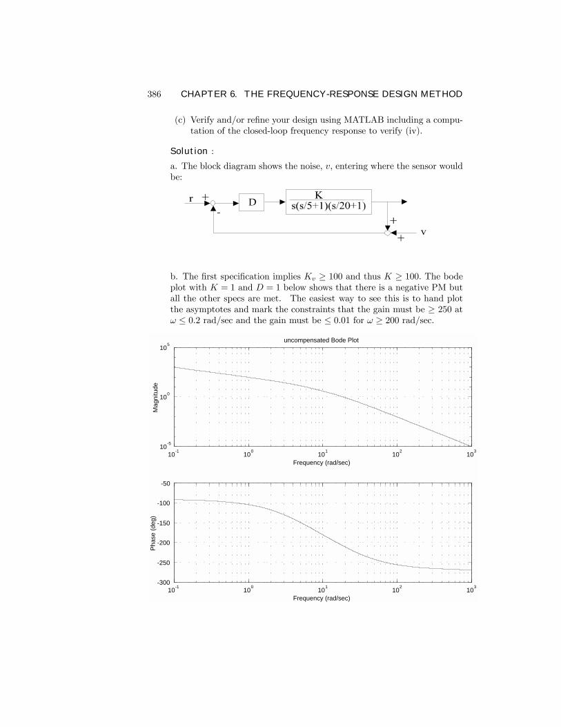
386 CHAPTER 6. THE FREQUENCY-RESPONSE DESIGN METHOD
(c) Verify and/or reÞne your design using MATLAB including a compu-tation of the closed-loop frequency response to verify (iv).
Solution :
a. The block diagram shows the noise, v, entering where the sensor wouldbe:
b. The Þrst speciÞcation implies Kv ≥ 100 and thus K ≥ 100. The bodeplot with K = 1 and D = 1 below shows that there is a negative PM butall the other specs are met. The easiest way to see this is to hand plotthe asymptotes and mark the constraints that the gain must be ≥ 250 atω ≤ 0.2 rad/sec and the gain must be ≤ 0.01 for ω ≥ 200 rad/sec.
10-1 100 101 102 10310-5
100
105
Frequency (rad/sec)
Mag
nitu
de
uncompensated Bode Plot
10-1 100 101 102 103-300
-250
-200
-150
-100
-50
Frequency (rad/sec)
Phas
e (d
eg)
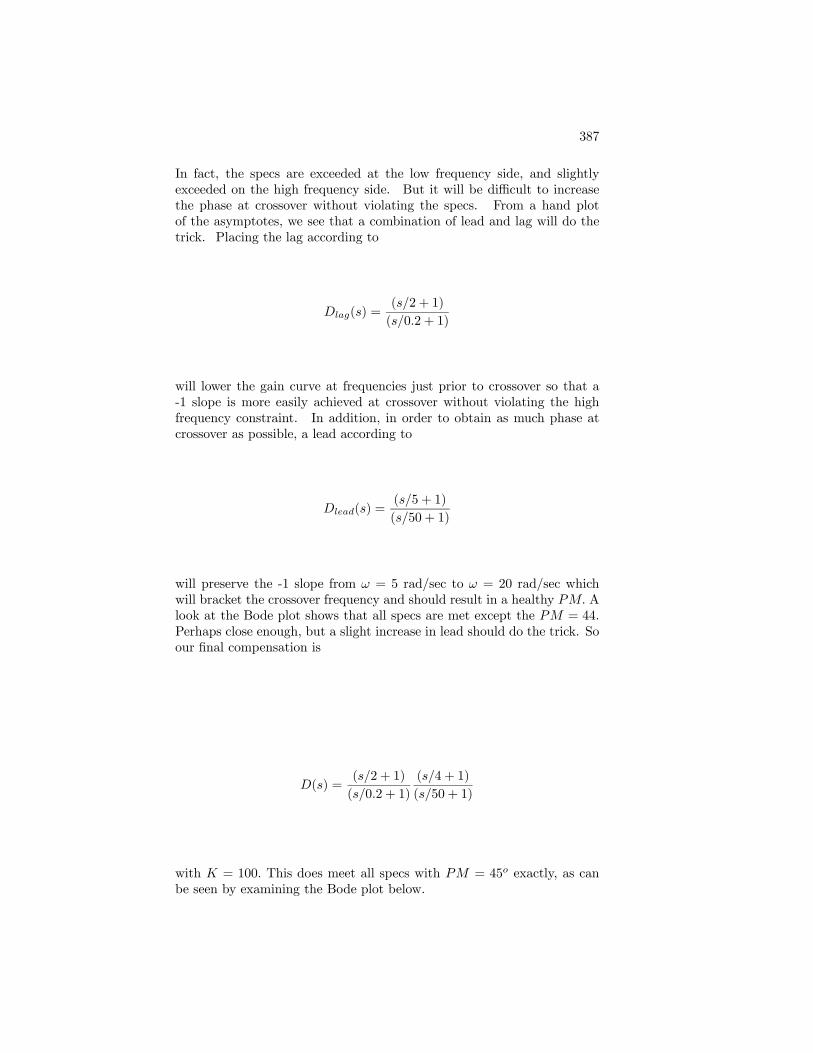
387
In fact, the specs are exceeded at the low frequency side, and slightlyexceeded on the high frequency side. But it will be difficult to increasethe phase at crossover without violating the specs. From a hand plotof the asymptotes, we see that a combination of lead and lag will do thetrick. Placing the lag according to
Dlag(s) =(s/2 + 1)
(s/0.2 + 1)
will lower the gain curve at frequencies just prior to crossover so that a-1 slope is more easily achieved at crossover without violating the highfrequency constraint. In addition, in order to obtain as much phase atcrossover as possible, a lead according to
Dlead(s) =(s/5 + 1)
(s/50 + 1)
will preserve the -1 slope from ω = 5 rad/sec to ω = 20 rad/sec whichwill bracket the crossover frequency and should result in a healthy PM. Alook at the Bode plot shows that all specs are met except the PM = 44.Perhaps close enough, but a slight increase in lead should do the trick. Soour Þnal compensation is
D(s) =(s/2 + 1)
(s/0.2 + 1)
(s/4 + 1)
(s/50 + 1)
with K = 100. This does meet all specs with PM = 45o exactly, as canbe seen by examining the Bode plot below.
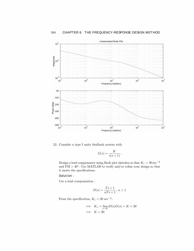
388 CHAPTER 6. THE FREQUENCY-RESPONSE DESIGN METHOD
10-1 100 101 102 10310-5
100
105
Frequency (rad/sec)
Mag
nitu
de
compensated Bode Plot
10-1 100 101 102 103-300
-250
-200
-150
-100
-50
Frequency (rad/sec)
Phas
e (d
eg)
52. Consider a type I unity feedback system with
G(s) =K
s(s+ 1).
Design a lead compensator using Bode plot sketches so thatKv = 20 sec−1
and PM > 40. Use MATLAB to verify and/or reÞne your design so thatit meets the speciÞcations.
Solution :
Use a lead compensation :
D(s) =Ts+ 1
αTs+ 1, α > 1
From the speciÞcation, Kv = 20 sec−1,
=⇒ Kv = lims→0
sD(s)G(s) = K = 20
=⇒ K = 20
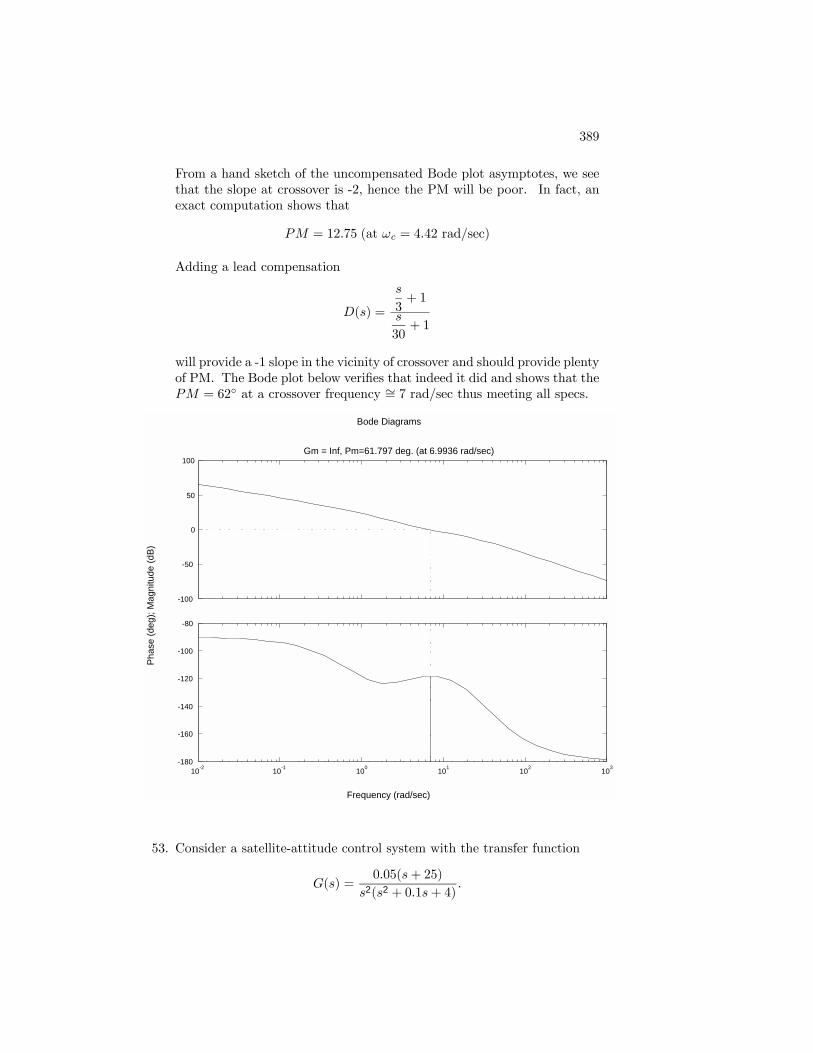
389
From a hand sketch of the uncompensated Bode plot asymptotes, we seethat the slope at crossover is -2, hence the PM will be poor. In fact, anexact computation shows that
PM = 12.75 (at ωc = 4.42 rad/sec)
Adding a lead compensation
D(s) =
s
3+ 1
s
30+ 1
will provide a -1 slope in the vicinity of crossover and should provide plentyof PM. The Bode plot below veriÞes that indeed it did and shows that thePM = 62 at a crossover frequency ∼= 7 rad/sec thus meeting all specs.
Frequency (rad/sec)
Phas
e (d
eg);
Mag
nitu
de (d
B)
Bode Diagrams
-100
-50
0
50
100Gm = Inf, Pm=61.797 deg. (at 6.9936 rad/sec)
10-2 10-1 100 101 102 103-180
-160
-140
-120
-100
-80
53. Consider a satellite-attitude control system with the transfer function
G(s) =0.05(s+ 25)
s2(s2 + 0.1s+ 4).
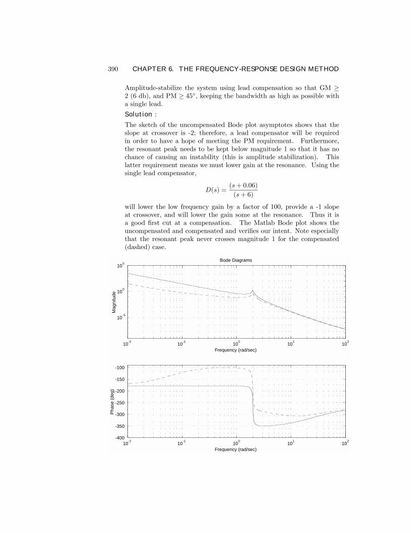
390 CHAPTER 6. THE FREQUENCY-RESPONSE DESIGN METHOD
Amplitude-stabilize the system using lead compensation so that GM ≥2 (6 db), and PM ≥ 45, keeping the bandwidth as high as possible witha single lead.
Solution :
The sketch of the uncompensated Bode plot asymptotes shows that theslope at crossover is -2; therefore, a lead compensator will be requiredin order to have a hope of meeting the PM requirement. Furthermore,the resonant peak needs to be kept below magnitude 1 so that it has nochance of causing an instability (this is amplitude stabilization). Thislatter requirement means we must lower gain at the resonance. Using thesingle lead compensator,
D(s) =(s+ 0.06)
(s+ 6)
will lower the low frequency gain by a factor of 100, provide a -1 slopeat crossover, and will lower the gain some at the resonance. Thus it isa good Þrst cut at a compensation. The Matlab Bode plot shows theuncompensated and compensated and veriÞes our intent. Note especiallythat the resonant peak never crosses magnitude 1 for the compensated(dashed) case.
10-2 10-1 100 101 102
10-5
100
105
Frequency (rad/sec)
Mag
nitu
de
Bode Diagrams
10-2 10-1 100 101 102-400
-350
-300
-250
-200
-150
-100
Frequency (rad/sec)
Phas
e (d
eg)
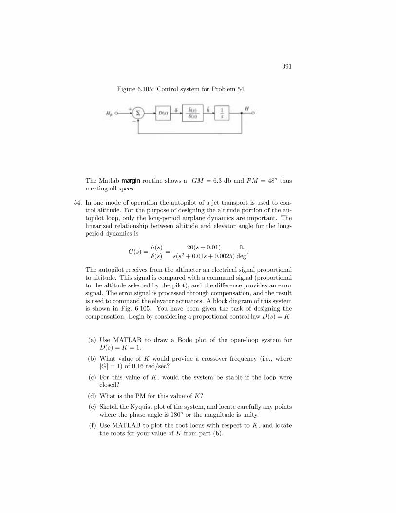
391
Figure 6.105: Control system for Problem 54
The Matlab margin routine shows a GM = 6.3 db and PM = 48 thusmeeting all specs.
54. In one mode of operation the autopilot of a jet transport is used to con-trol altitude. For the purpose of designing the altitude portion of the au-topilot loop, only the long-period airplane dynamics are important. Thelinearized relationship between altitude and elevator angle for the long-period dynamics is
G(s) =h(s)
δ(s)=
20(s+ 0.01)
s(s2 + 0.01s+ 0.0025)
ft
deg.
The autopilot receives from the altimeter an electrical signal proportionalto altitude. This signal is compared with a command signal (proportionalto the altitude selected by the pilot), and the difference provides an errorsignal. The error signal is processed through compensation, and the resultis used to command the elevator actuators. A block diagram of this systemis shown in Fig. 6.105. You have been given the task of designing thecompensation. Begin by considering a proportional control law D(s) = K.
(a) Use MATLAB to draw a Bode plot of the open-loop system forD(s) = K = 1.
(b) What value of K would provide a crossover frequency (i.e., where|G| = 1) of 0.16 rad/sec?
(c) For this value of K, would the system be stable if the loop wereclosed?
(d) What is the PM for this value of K?
(e) Sketch the Nyquist plot of the system, and locate carefully any pointswhere the phase angle is 180 or the magnitude is unity.
(f) Use MATLAB to plot the root locus with respect to K, and locatethe roots for your value of K from part (b).
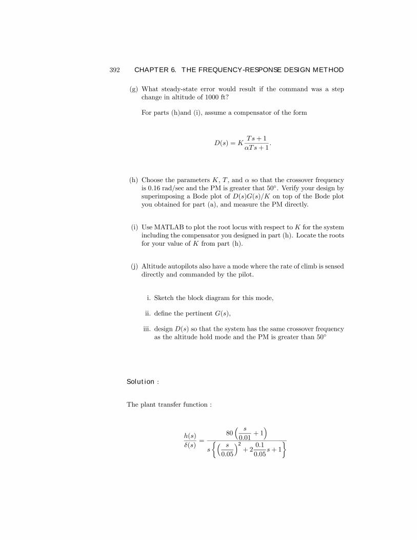
392 CHAPTER 6. THE FREQUENCY-RESPONSE DESIGN METHOD
(g) What steady-state error would result if the command was a stepchange in altitude of 1000 ft?
For parts (h)and (i), assume a compensator of the form
D(s) = KTs+ 1
αTs+ 1.
(h) Choose the parameters K, T , and α so that the crossover frequencyis 0.16 rad/sec and the PM is greater that 50. Verify your design bysuperimposing a Bode plot of D(s)G(s)/K on top of the Bode plotyou obtained for part (a), and measure the PM directly.
(i) Use MATLAB to plot the root locus with respect to K for the systemincluding the compensator you designed in part (h). Locate the rootsfor your value of K from part (h).
(j) Altitude autopilots also have a mode where the rate of climb is senseddirectly and commanded by the pilot.
i. Sketch the block diagram for this mode,
ii. deÞne the pertinent G(s),
iii. design D(s) so that the system has the same crossover frequencyas the altitude hold mode and the PM is greater than 50
Solution :
The plant transfer function :
h(s)
δ(s)=
80³ s
0.01+ 1´
s
½³ s
0.05
´2
+ 20.1
0.05s+ 1
¾
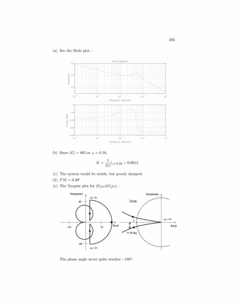
393
(a) See the Bode plot :
10-4
10-3
10-2
10-1
100
102
104
106
Frequency (rad/sec)
Magnitude
B ode D iagram s
10-4
10-3
10-2
10-1
100
-200
-150
-100
-50
0
Frequency (rad/sec)
Phase (deg)
(b) Since |G| = 865 at ω = 0.16,
K =1
|G| |ω=0.16 = 0.0012
(c) The system would be stable, but poorly damped.
(d) PM = 0.39
(e) The Nyquist plot for D(jω)G(jω) :
The phase angle never quite reaches −180.
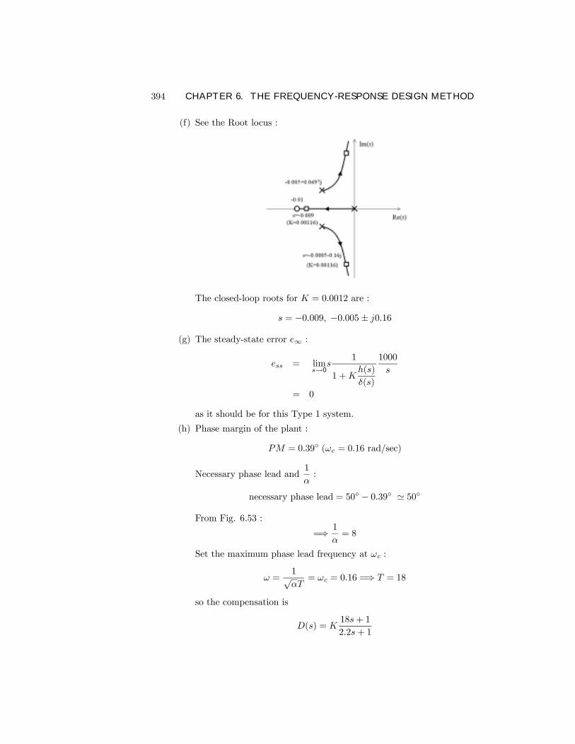
394 CHAPTER 6. THE FREQUENCY-RESPONSE DESIGN METHOD
(f) See the Root locus :
The closed-loop roots for K = 0.0012 are :
s = −0.009, −0.005± j0.16
(g) The steady-state error e∞ :
ess = lims→0
s1
1 +Kh(s)
δ(s)
1000
s
= 0
as it should be for this Type 1 system.
(h) Phase margin of the plant :
PM = 0.39 (ωc = 0.16 rad/sec)
Necessary phase lead and1
α:
necessary phase lead = 50 − 0.39 ' 50
From Fig. 6.53 :
=⇒ 1
α= 8
Set the maximum phase lead frequency at ωc :
ω =1√αT
= ωc = 0.16 =⇒ T = 18
so the compensation is
D(s) = K18s+ 1
2.2s+ 1
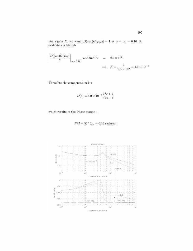
395
For a gain K, we want |D(jωc)G(jωc)| = 1 at ω = ωc = 0.16. Soevaluate via Matlab
¯D(jωc)G(jωc)
K
¯ωc=0.16
and Þnd it = 2.5× 103
=⇒ K =1
2.5× 103= 4.0× 10⁻⁴
Therefore the compensation is :
D(s) = 4.0× 10⁻⁴ 18s+ 1
2.2s+ 1
which results in the Phase margin :
PM = 52 (ωc = 0.16 rad/sec)
10-3
10-2
10-1
100
102
104
106
Frequency (rad/sec)
Magnitude
B ode D iagram s
10-3
10-2
10-1
100
-200
-150
-100
-50
0
Frequency (rad/sec)
Phase (deg)
51.4 deg -180 deg
G D G /K D G /K
K=4.09x10⁻⁴
w =0.16
G
D G /K
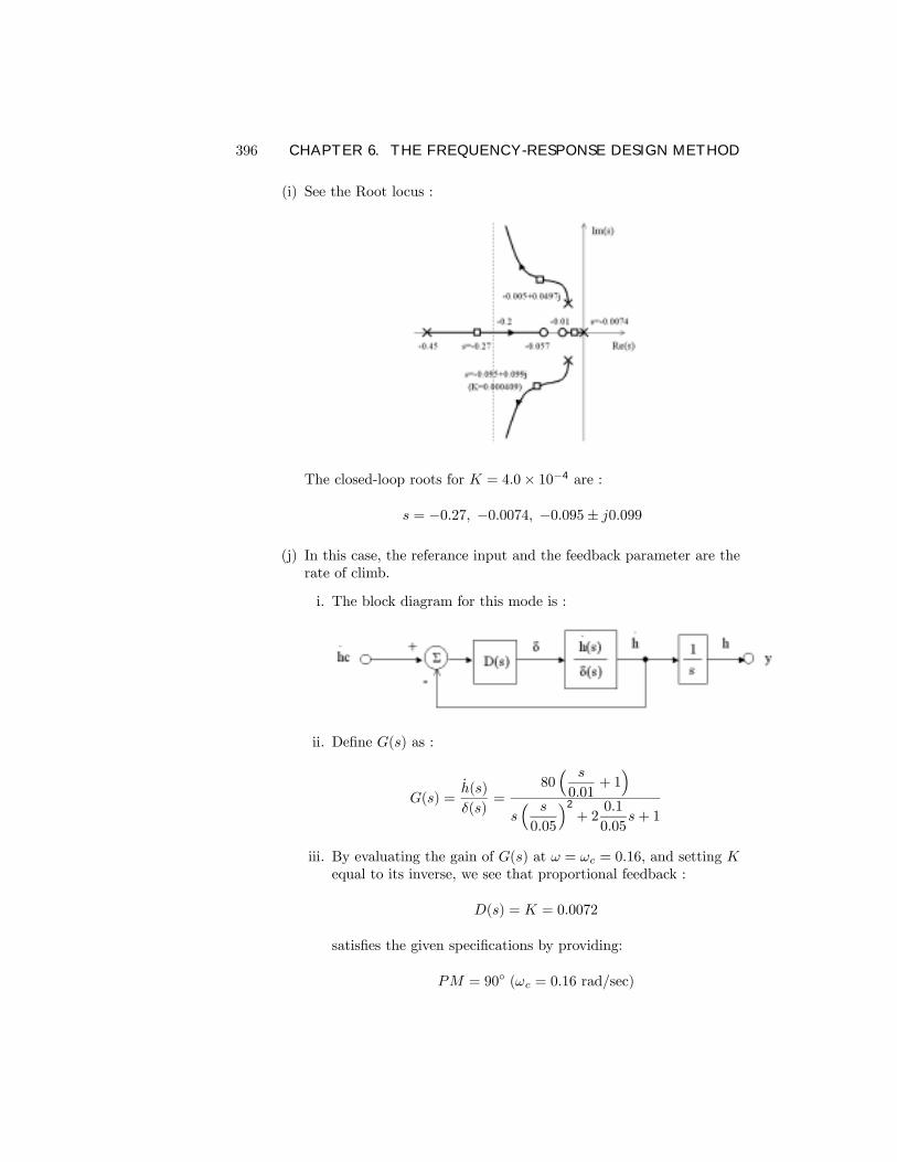
396 CHAPTER 6. THE FREQUENCY-RESPONSE DESIGN METHOD
(i) See the Root locus :
The closed-loop roots for K = 4.0× 10⁻⁴ are :
s = −0.27, −0.0074, −0.095± j0.099
(j) In this case, the referance input and the feedback parameter are therate of climb.
i. The block diagram for this mode is :
ii. DeÞne G(s) as :
G(s) =úh(s)
δ(s)=
80³ s
0.01+ 1´
s³ s
0.05
´2
+ 20.1
0.05s+ 1
iii. By evaluating the gain of G(s) at ω = ωc = 0.16, and setting Kequal to its inverse, we see that proportional feedback :
D(s) = K = 0.0072
satisÞes the given speciÞcations by providing:
PM = 90 (ωc = 0.16 rad/sec)
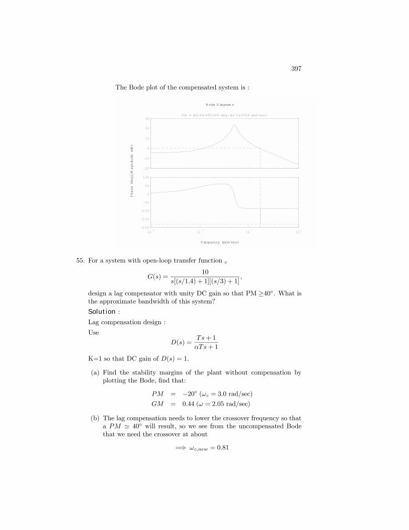
397
The Bode plot of the compensated system is :
Frequency (rad/sec)
Phase (deg); M
agnitude (dB)
B ode D iagram s
-20
-10
0
10
20
30G m = Inf, Pm =90.349 deg. (at 0.16509 rad/sec)
10-3
10-2
10-1
100
-200
-150
-100
-50
0
50
100
55. For a system with open-loop transfer function c
G(s) =10
s[(s/1.4) + 1][(s/3) + 1],
design a lag compensator with unity DC gain so that PM ≥40. What isthe approximate bandwidth of this system?
Solution :
Lag compensation design :
Use
D(s) =Ts+ 1
αTs+ 1
K=1 so that DC gain of D(s) = 1.
(a) Find the stability margins of the plant without compensation byplotting the Bode, Þnd that:
PM = −20 (ωc = 3.0 rad/sec)GM = 0.44 (ω = 2.05 rad/sec)
(b) The lag compensation needs to lower the crossover frequency so thata PM ' 40 will result, so we see from the uncompensated Bodethat we need the crossover at about
=⇒ ωc,new = 0.81
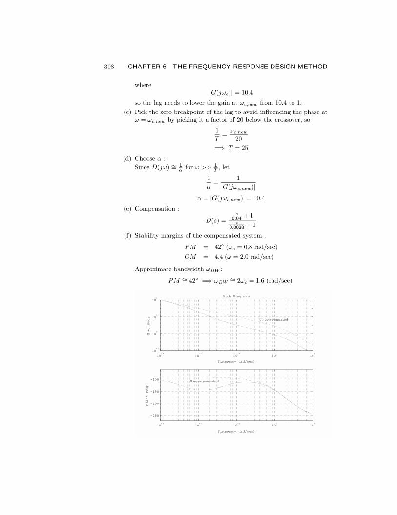
398 CHAPTER 6. THE FREQUENCY-RESPONSE DESIGN METHOD
where|G(jωc)| = 10.4
so the lag needs to lower the gain at ωc,new from 10.4 to 1.
(c) Pick the zero breakpoint of the lag to avoid inßuencing the phase atω = ωc,new by picking it a factor of 20 below the crossover, so
1
T=ωc,new20
=⇒ T = 25
(d) Choose α :
Since D(jω) ∼= 1α for ω >>
1T , let
1
α=
1
|G(jωc,new)|α = |G(jωc,new)| = 10.4
(e) Compensation :
D(s) =s
0.04 + 1s
0.0038 + 1
(f) Stability margins of the compensated system :
PM = 42 (ωc = 0.8 rad/sec)GM = 4.4 (ω = 2.0 rad/sec)
Approximate bandwidth ωBW :
PM ∼= 42 =⇒ ωBW ∼= 2ωc = 1.6 (rad/sec)
10-3
10-2
10-1
100
101
10-2
100
102
104
Frequency (rad/sec)
Magnitude
B ode D iagram s
U ncom pensated
10-3
10-2
10-1
100
101
-250
-200
-150
-100
Frequency (rad/sec)
Phase (deg)
U ncom pensated
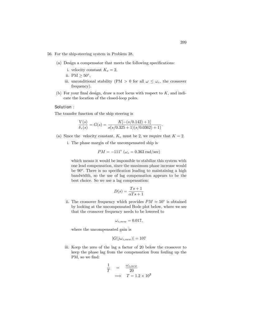
399
56. For the ship-steering system in Problem 38,
(a) Design a compensator that meets the following speciÞcations:
i. velocity constant Kv = 2,
ii. PM ≥ 50,iii. unconditional stability (PM > 0 for all ω ≤ ωc, the crossover
frequency).
(b) For your Þnal design, draw a root locus with respect to K, and indi-cate the location of the closed-loop poles.
Solution :
The transfer function of the ship steering is
V (s)
δr(s)= G(s) =
K[−(s/0.142) + 1]s(s/0.325 + 1)(s/0.0362) + 1)
.
(a) Since the velocity constant, Kv must be 2, we require that K = 2.
i. The phase margin of the uncompensated ship is
PM = −111 (ωc = 0.363 rad/sec)which means it would be impossible to stabilize this system withone lead compensation, since the maximum phase increase wouldbe 90o. There is no speciÞcation leading to maintaining a highbandwidth, so the use of lag compensation appears to be thebest choice. So we use a lag compensation:
D(s) =Ts+ 1
αTs+ 1
ii. The crossover frequency which provides PM ' 50 is obtainedby looking at the uncompensated Bode plot below, where we seethat the crossover frequency needs to be lowered to
ωc,new = 0.017,
where the uncompensated gain is
|G(jωc,new)| = 107iii. Keep the zero of the lag a factor of 20 below the crossover to
keep the phase lag from the compensation from fouling up thePM, so we Þnd:
1
T=
ωc,new20
=⇒ T = 1.2× 10³
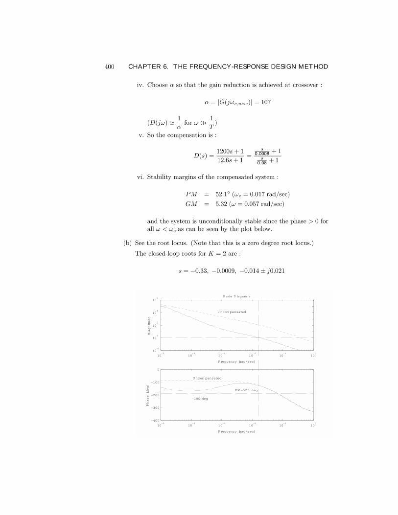
400 CHAPTER 6. THE FREQUENCY-RESPONSE DESIGN METHOD
iv. Choose α so that the gain reduction is achieved at crossover :
α = |G(jωc,new)| = 107
(D(jω) ' 1
αfor ω À 1
T)
v. So the compensation is :
D(s) =1200s+ 1
12.6s+ 1=
s0.0008 + 1s
0.08 + 1
vi. Stability margins of the compensated system :
PM = 52.1 (ωc = 0.017 rad/sec)GM = 5.32 (ω = 0.057 rad/sec)
and the system is unconditionally stable since the phase > 0 forall ω < ωc.as can be seen by the plot below.
(b) See the root locus. (Note that this is a zero degree root locus.)
The closed-loop roots for K = 2 are :
s = −0.33, −0.0009, −0.014± j0.021
10-5
10-4
10-3
10-2
10-1
100
10-2
100
102
104
106
Frequency (rad/sec)
Magnitude
B ode D iagram s
10-5
10-4
10-3
10-2
10-1
100
-400
-300
-200
-100
0
Frequency (rad/sec)
Phase (deg)
U ncom pensated
-180 deg
U ncom pensated
PM =52.1 deg
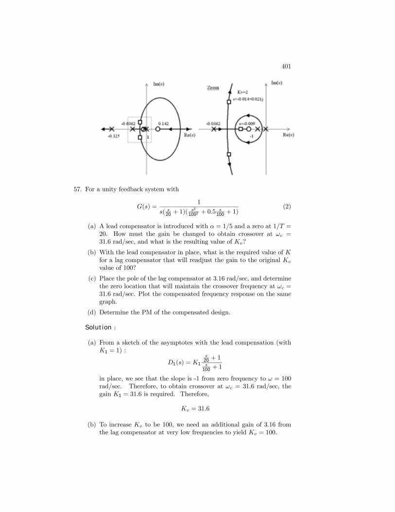
401
57. For a unity feedback system with
G(s) =1
s( s20 + 1)(s2
1002 + 0.5s
100 + 1)(2)
(a) A lead compensator is introduced with α = 1/5 and a zero at 1/T =20. How must the gain be changed to obtain crossover at ωc =31.6 rad/sec, and what is the resulting value of Kv?
(b) With the lead compensator in place, what is the required value of Kfor a lag compensator that will readjust the gain to the original Kv
value of 100?
(c) Place the pole of the lag compensator at 3.16 rad/sec, and determinethe zero location that will maintain the crossover frequency at ωc =31.6 rad/sec. Plot the compensated frequency response on the samegraph.
(d) Determine the PM of the compensated design.
Solution :
(a) From a sketch of the asymptotes with the lead compensation (withK1 = 1) :
D1(s) = K1
s20 + 1s
100 + 1
in place, we see that the slope is -1 from zero frequency to ω = 100rad/sec. Therefore, to obtain crossover at ωc = 31.6 rad/sec, thegain K1 = 31.6 is required. Therefore,
Kv = 31.6
(b) To increase Kv to be 100, we need an additional gain of 3.16 fromthe lag compensator at very low frequencies to yield Kv = 100.
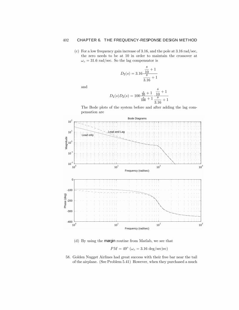
402 CHAPTER 6. THE FREQUENCY-RESPONSE DESIGN METHOD
(c) For a low frequency gain increase of 3.16, and the pole at 3.16 rad/sec,the zero needs to be at 10 in order to maintain the crossover atωc = 31.6 rad/sec. So the lag compensator is
D2(s) = 3.16
s
10+ 1
s
3.16+ 1
and
D1(s)D2(s) = 100s
20 + 1s
100 + 1
s
10+ 1
s
3.16+ 1
The Bode plots of the system before and after adding the lag com-pensation are
100 101 102 10310-2
10-1
100
101
102
Frequency (rad/sec)
Mag
nitu
de
Bode Diagrams
Lead and LagLead only
100 101 102 103-400
-300
-200
-100
0
Frequency (rad/sec)
Phas
e (d
eg)
(d) By using the margin routine from Matlab, we see that
PM = 49 (ωc = 3.16 deg/sec)ec)
58. Golden Nugget Airlines had great success with their free bar near the tailof the airplane. (See Problem 5.41) However, when they purchased a much
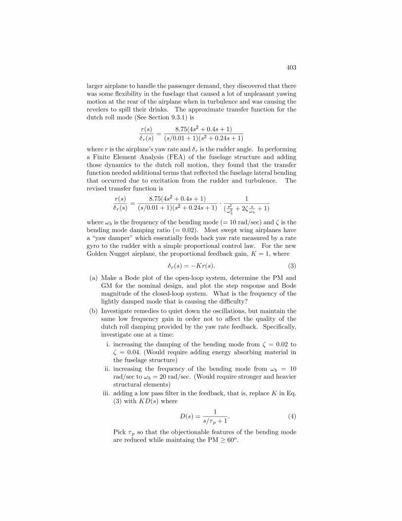
403
larger airplane to handle the passenger demand, they discovered that therewas some ßexibility in the fuselage that caused a lot of unpleasant yawingmotion at the rear of the airplane when in turbulence and was causing therevelers to spill their drinks. The approximate transfer function for thedutch roll mode (See Section 9.3.1) is
r(s)
δr(s)=
8.75(4s2 + 0.4s+ 1)
(s/0.01 + 1)(s2 + 0.24s+ 1)
where r is the airplanes yaw rate and δr is the rudder angle. In performinga Finite Element Analysis (FEA) of the fuselage structure and addingthose dynamics to the dutch roll motion, they found that the transferfunction needed additional terms that reßected the fuselage lateral bendingthat occurred due to excitation from the rudder and turbulence. Therevised transfer function is
r(s)
δr(s)=
8.75(4s2 + 0.4s+ 1)
(s/0.01 + 1)(s2 + 0.24s+ 1)· 1
( s2
ω2b+ 2ζ s
ωb+ 1)
where ωb is the frequency of the bending mode (= 10 rad/sec) and ζ is thebending mode damping ratio (= 0.02). Most swept wing airplanes havea yaw damper which essentially feeds back yaw rate measured by a rategyro to the rudder with a simple proportional control law. For the newGolden Nugget airplane, the proportional feedback gain, K = 1, where
δr(s) = −Kr(s). (3)
(a) Make a Bode plot of the open-loop system, determine the PM andGM for the nominal design, and plot the step response and Bodemagnitude of the closed-loop system. What is the frequency of thelightly damped mode that is causing the difficulty?
(b) Investigate remedies to quiet down the oscillations, but maintain thesame low frequency gain in order not to affect the quality of thedutch roll damping provided by the yaw rate feedback. SpeciÞcally,investigate one at a time:
i. increasing the damping of the bending mode from ζ = 0.02 toζ = 0.04. (Would require adding energy absorbing material inthe fuselage structure)
ii. increasing the frequency of the bending mode from ωb = 10rad/sec to ωb = 20 rad/sec. (Would require stronger and heavierstructural elements)
iii. adding a low pass Þlter in the feedback, that is, replace K in Eq.(3) with KD(s) where
D(s) =1
s/τp + 1. (4)
Pick τp so that the objectionable features of the bending modeare reduced while maintaing the PM ≥ 60o.
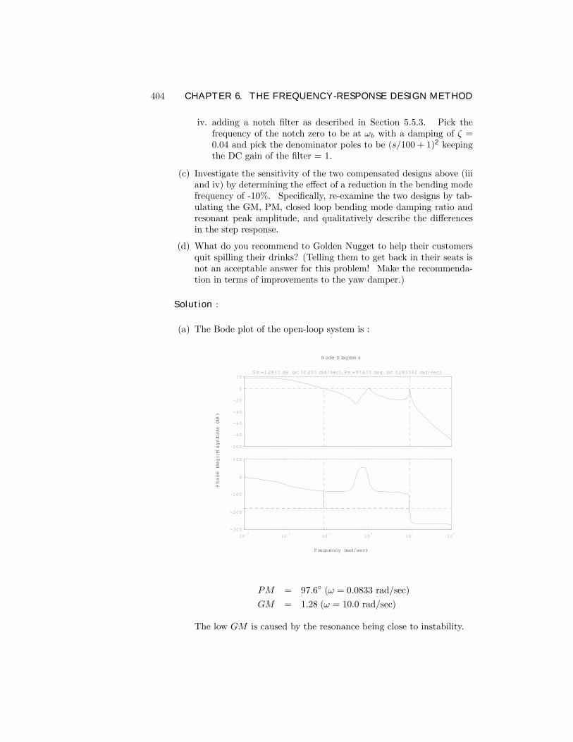
404 CHAPTER 6. THE FREQUENCY-RESPONSE DESIGN METHOD
iv. adding a notch Þlter as described in Section 5.5.3. Pick thefrequency of the notch zero to be at ωb with a damping of ζ =0.04 and pick the denominator poles to be (s/100 + 1)2 keepingthe DC gain of the Þlter = 1.
(c) Investigate the sensitivity of the two compensated designs above (iiiand iv) by determining the effect of a reduction in the bending modefrequency of -10%. SpeciÞcally, re-examine the two designs by tab-ulating the GM, PM, closed loop bending mode damping ratio andresonant peak amplitude, and qualitatively describe the differencesin the step response.
(d) What do you recommend to Golden Nugget to help their customersquit spilling their drinks? (Telling them to get back in their seats isnot an acceptable answer for this problem! Make the recommenda-tion in terms of improvements to the yaw damper.)
Solution :
(a) The Bode plot of the open-loop system is :
Frequency (rad/sec)
Phase (deg); M
agnitude (dB)
B ode D iagram s
-100
-80
-60
-40
-20
0
20G m =1.2833 dB (at 10.003 rad/sec), Pm =97.633 deg. (at 0.083342 rad/sec)
10-3
10-2
10-1
100
101
102
-300
-200
-100
0
100
PM = 97.6 (ω = 0.0833 rad/sec)GM = 1.28 (ω = 10.0 rad/sec)
The low GM is caused by the resonance being close to instability.
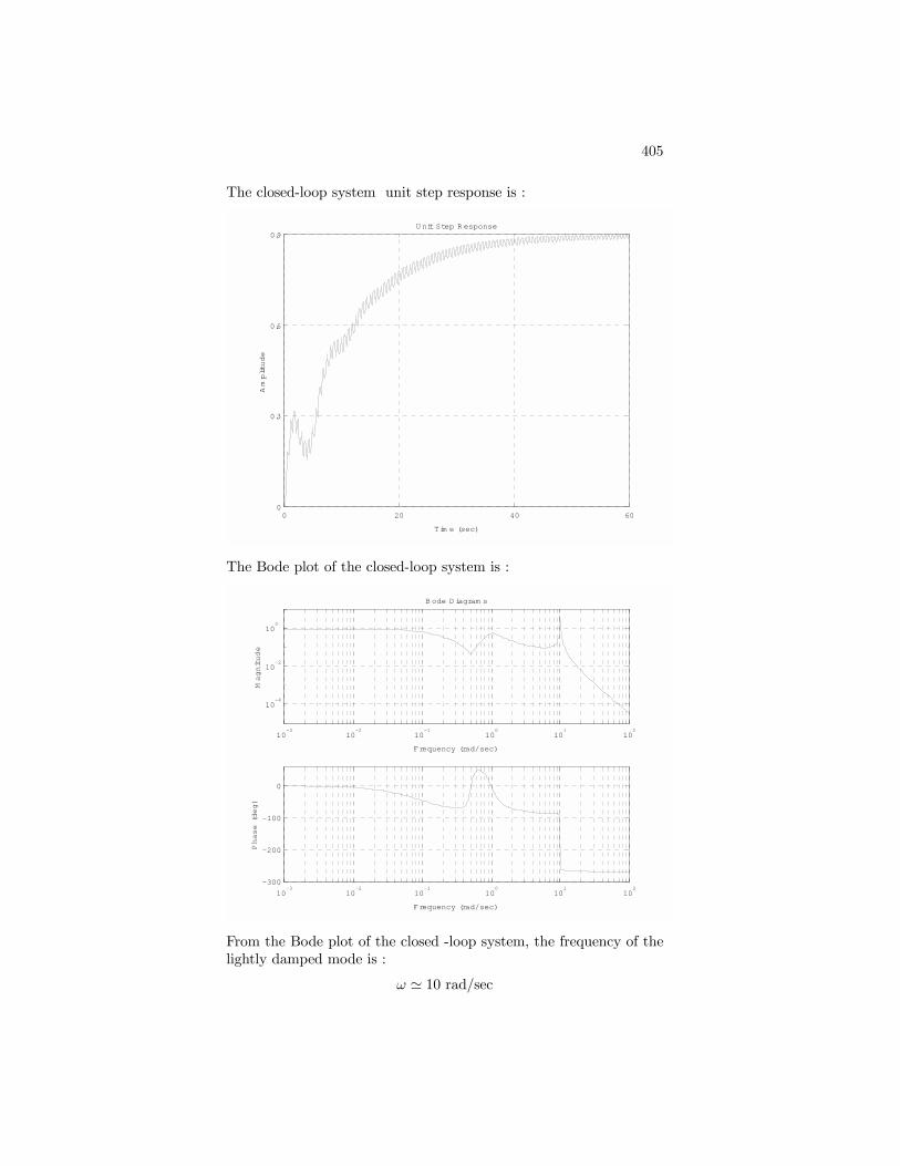
405
The closed-loop system unit step response is :
0 20 40 600
0.3
0.6
0.9
Tim e (sec)
Amplitude
U nit Step R esponse
The Bode plot of the closed-loop system is :
10-3
10-2
10-1
100
101
102
10-4
10-2
100
Frequency (rad/sec)
Magnitude
B ode D iagram s
10-3
10-2
10-1
100
101
102
-300
-200
-100
0
Frequency (rad/sec)
Phase (deg)
From the Bode plot of the closed -loop system, the frequency of thelightly damped mode is :
ω ' 10 rad/sec
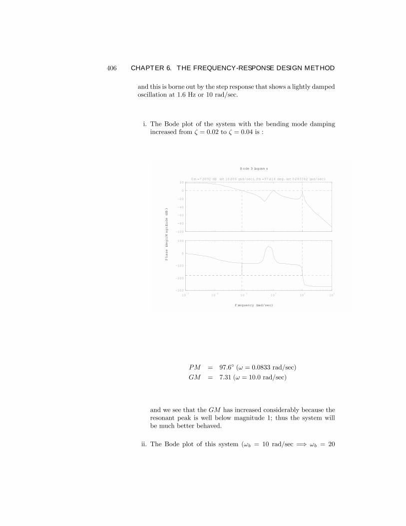
406 CHAPTER 6. THE FREQUENCY-RESPONSE DESIGN METHOD
and this is borne out by the step response that shows a lightly dampedoscillation at 1.6 Hz or 10 rad/sec.
i. The Bode plot of the system with the bending mode dampingincreased from ζ = 0.02 to ζ = 0.04 is :
Frequency (rad/sec)
Phase (deg); M
agnitude (dB)
B ode D iagram s
-100
-80
-60
-40
-20
0
20G m =7.3092 dB (at 10.006 rad/sec), Pm =97.614 deg. (at 0.083342 rad/sec)
10-3
10-2
10-1
100
101
102
-300
-200
-100
0
100
PM = 97.6 (ω = 0.0833 rad/sec)GM = 7.31 (ω = 10.0 rad/sec)
and we see that the GM has increased considerably because theresonant peak is well below magnitude 1; thus the system willbe much better behaved.
ii. The Bode plot of this system (ωb = 10 rad/sec =⇒ ωb = 20
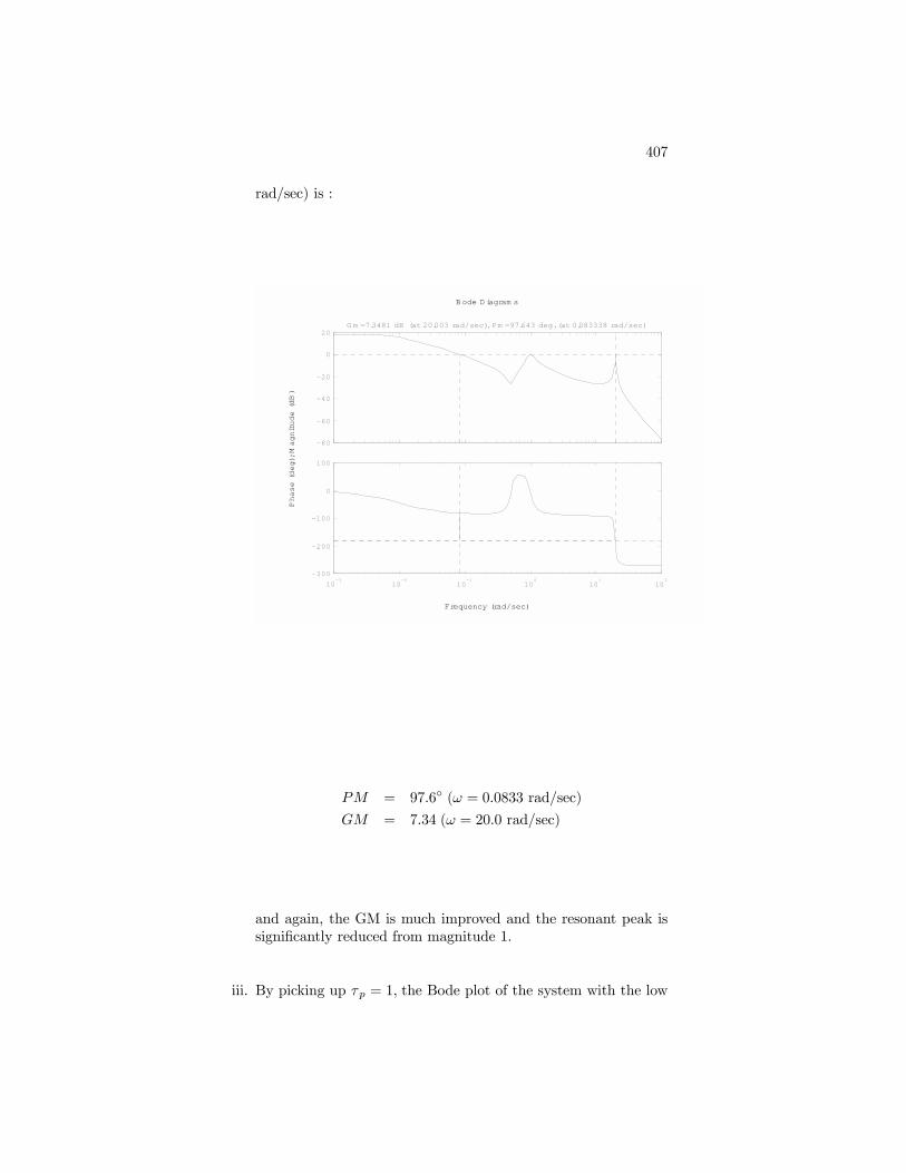
407
rad/sec) is :
Frequency (rad/sec)
Phase (deg); M
agnitude (dB)
B ode D iagram s
-80
-60
-40
-20
0
20G m =7.3481 dB (at 20.003 rad/sec), Pm =97.643 deg. (at 0.083338 rad/sec)
10-3
10-2
10-1
100
101
102
-300
-200
-100
0
100
PM = 97.6 (ω = 0.0833 rad/sec)GM = 7.34 (ω = 20.0 rad/sec)
and again, the GM is much improved and the resonant peak issigniÞcantly reduced from magnitude 1.
iii. By picking up τp = 1, the Bode plot of the system with the low
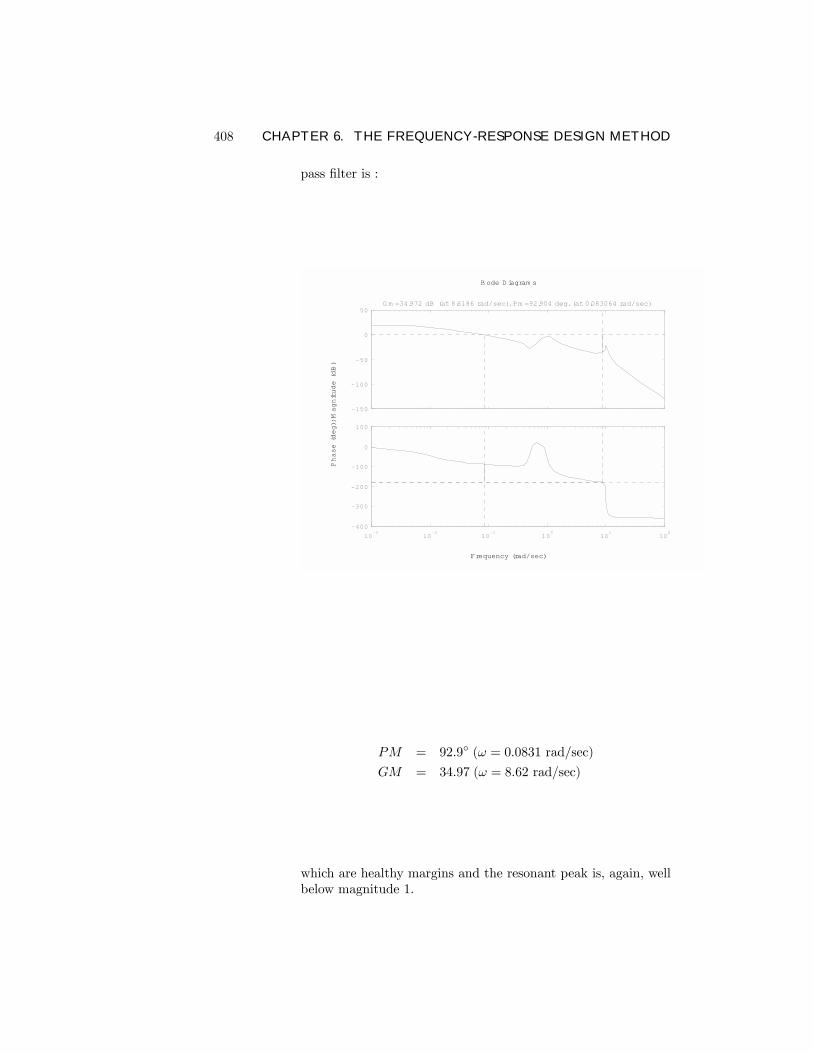
408 CHAPTER 6. THE FREQUENCY-RESPONSE DESIGN METHOD
pass Þlter is :
Frequency (rad/sec)
Phase (deg); M
agnitude (dB)
B ode D iagram s
-150
-100
-50
0
50G m =34.972 dB (at 8.6186 rad/sec), Pm =92.904 deg. (at 0.083064 rad/sec)
10-3
10-2
10-1
100
101
102
-400
-300
-200
-100
0
100
PM = 92.9 (ω = 0.0831 rad/sec)GM = 34.97 (ω = 8.62 rad/sec)
which are healthy margins and the resonant peak is, again, wellbelow magnitude 1.
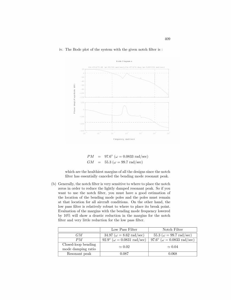
409
iv. The Bode plot of the system with the given notch Þlter is :
Frequency (rad/sec)
Phase (deg); M
agnitude (dB)
B ode D iagram s
-120
-100
-80
-60
-40
-20
0
20G m =55.275 dB (at 99.746 rad/sec), Pm =97.576 deg. (at 0.083336 rad/sec)
10-3
10-2
10-1
100
101
102
103
-300
-200
-100
0
100
PM = 97.6 (ω = 0.0833 rad/sec)GM = 55.3 (ω = 99.7 rad/sec)
which are the healthiest margins of all the designs since the notchÞlter has essentially canceled the bending mode resonant peak.
(b) Generally, the notch Þlter is very sensitive to where to place the notchzeros in order to reduce the lightly damped resonant peak. So if youwant to use the notch Þlter, you must have a good estimation ofthe location of the bending mode poles and the poles must remainat that location for all aircraft conditions. On the other hand, thelow pass Þlter is relatively robust to where to place its break point.Evaluation of the margins with the bending mode frequency loweredby 10% will show a drastic reduction in the margins for the notchÞlter and very little reduction for the low pass Þlter.
Low Pass Filter Notch Filter
GM 34.97 (ω = 8.62 rad/sec) 55.3 (ω = 99.7 rad/sec)PM 92.9 (ω = 0.0831 rad/sec) 97.6 (ω = 0.0833 rad/sec)
Closed-loop bendingmode damping ratio
' 0.02 ' 0.04Resonant peak 0.087 0.068
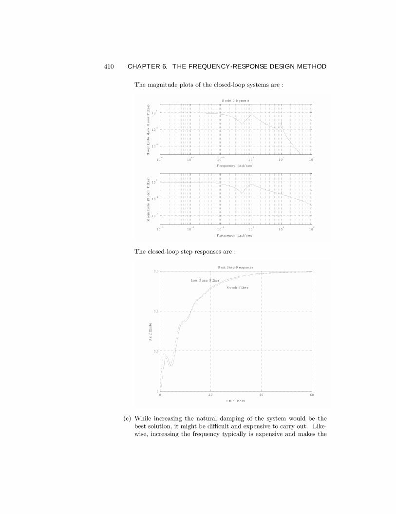
410 CHAPTER 6. THE FREQUENCY-RESPONSE DESIGN METHOD
The magnitude plots of the closed-loop systems are :
10-3
10-2
10-1
100
101
102
10-4
10-2
100
Frequency (rad/sec)
Magnitude (Low Pass Filter)
B ode D iagram s
10-3
10-2
10-1
100
101
102
10-4
10-2
100
Frequency (rad/sec)
Magnitude (Notch Filter)
The closed-loop step responses are :
0 20 40 600
0.3
0.6
0.9
Tim e (sec)
Amplitude
U nit Step R esponse
N otch Filter
Low Pass Filter
(c) While increasing the natural damping of the system would be thebest solution, it might be difficult and expensive to carry out. Like-wise, increasing the frequency typically is expensive and makes the
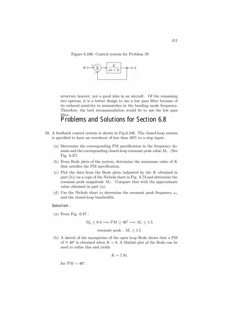
411
Figure 6.106: Control system for Problem 59
structure heavier, not a good idea in an aircraft. Of the remainingtwo options, it is a better design to use a low pass Þlter because ofits reduced sensivity to mismatches in the bending mode frequency.Therefore, the best recommendation would be to use the low passÞlter.
Problems and Solutions for Section 6.8
59. A feedback control system is shown in Fig.6.106. The closed-loop systemis speciÞed to have an overshoot of less than 30% to a step input.
(a) Determine the corresponding PM speciÞcation in the frequency do-main and the corresponding closed-loop resonant peak valueMr. (SeeFig. 6.37)
(b) From Bode plots of the system, determine the maximum value of Kthat satisÞes the PM speciÞcation.
(c) Plot the data from the Bode plots (adjusted by the K obtained inpart (b)) on a copy of the Nichols chart in Fig. 6.73 and determine theresonant peak magnitude Mr. Compare that with the approximatevalue obtained in part (a).
(d) Use the Nichols chart to determine the resonant peak frequency ωrand the closed-loop bandwidth.
Solution :
(a) From Fig. 6.37 :
Mp ≤ 0.3 =⇒ PM ≥ 40o =⇒Mr ≤ 1.5resonant peak : Mr ≤ 1.5
(b) A sketch of the asymptotes of the open loop Bode shows that a PMof ∼= 40o is obtained when K = 8. A Matlab plot of the Bode can beused to reÞne this and yields
K = 7.81
for PM = 40o.
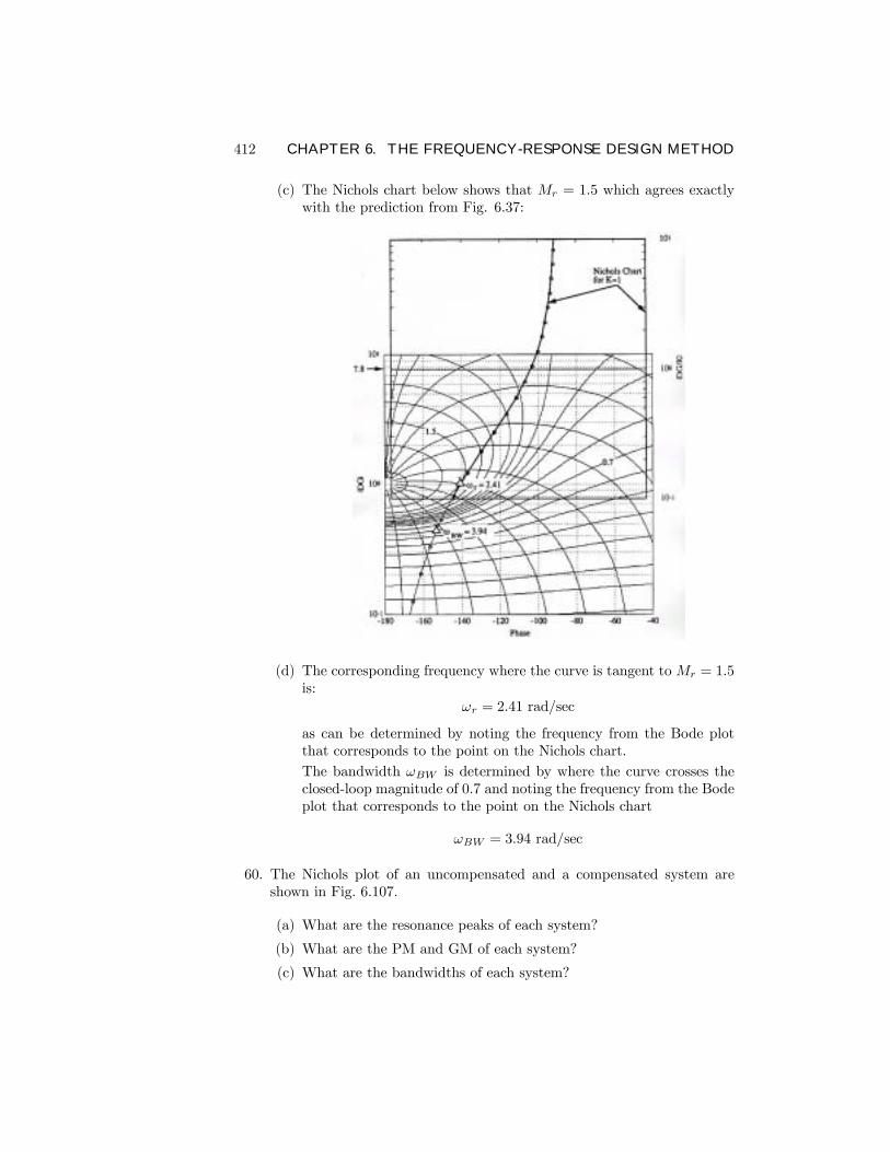
412 CHAPTER 6. THE FREQUENCY-RESPONSE DESIGN METHOD
(c) The Nichols chart below shows that Mr = 1.5 which agrees exactlywith the prediction from Fig. 6.37:
(d) The corresponding frequency where the curve is tangent toMr = 1.5is:
ωr = 2.41 rad/sec
as can be determined by noting the frequency from the Bode plotthat corresponds to the point on the Nichols chart.
The bandwidth ωBW is determined by where the curve crosses theclosed-loop magnitude of 0.7 and noting the frequency from the Bodeplot that corresponds to the point on the Nichols chart
ωBW = 3.94 rad/sec
60. The Nichols plot of an uncompensated and a compensated system areshown in Fig. 6.107.
(a) What are the resonance peaks of each system?
(b) What are the PM and GM of each system?
(c) What are the bandwidths of each system?
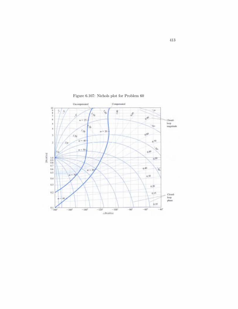
413
Figure 6.107: Nichols plot for Problem 60
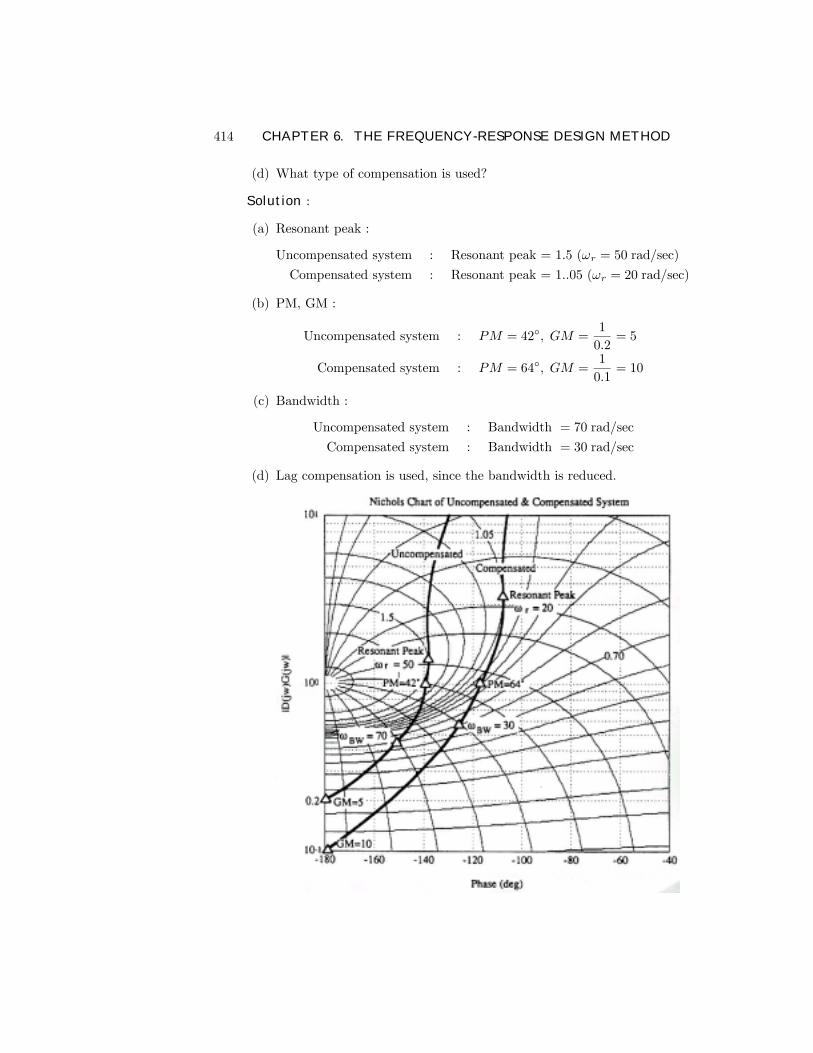
414 CHAPTER 6. THE FREQUENCY-RESPONSE DESIGN METHOD
(d) What type of compensation is used?
Solution :
(a) Resonant peak :
Uncompensated system : Resonant peak = 1.5 (ωr = 50 rad/sec)
Compensated system : Resonant peak = 1..05 (ωr = 20 rad/sec)
(b) PM, GM :
Uncompensated system : PM = 42, GM =1
0.2= 5
Compensated system : PM = 64, GM =1
0.1= 10
(c) Bandwidth :
Uncompensated system : Bandwidth = 70 rad/sec
Compensated system : Bandwidth = 30 rad/sec
(d) Lag compensation is used, since the bandwidth is reduced.
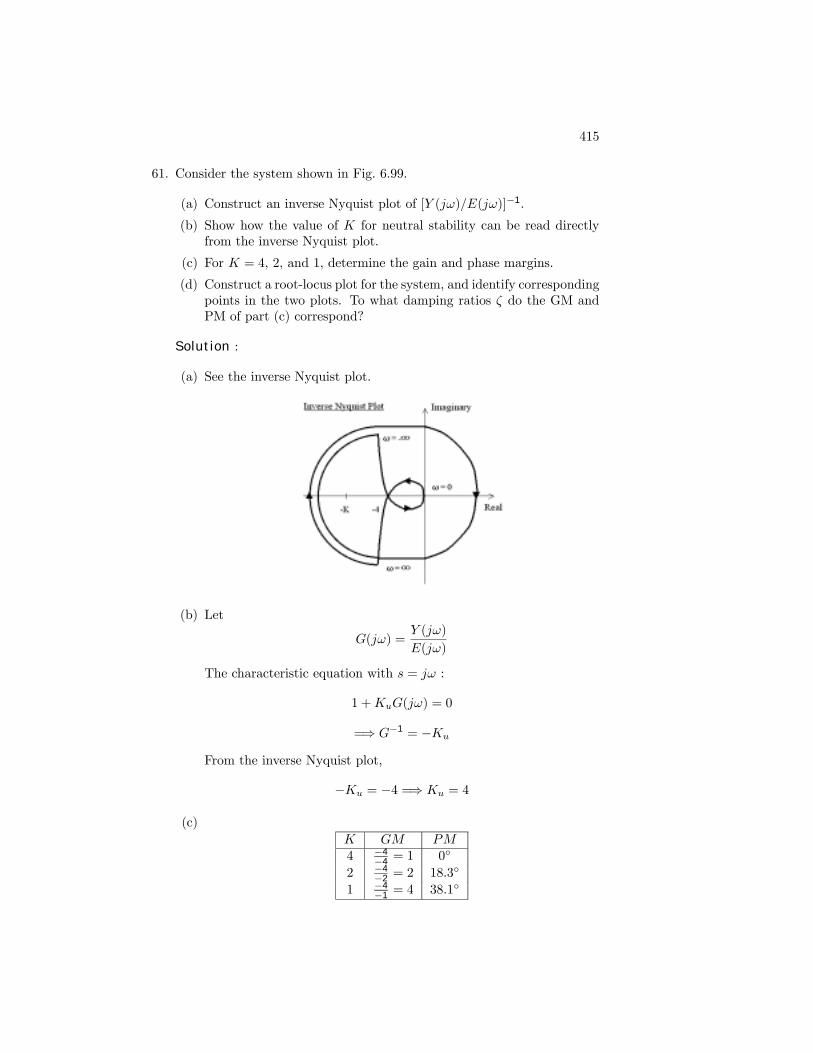
415
61. Consider the system shown in Fig. 6.99.
(a) Construct an inverse Nyquist plot of [Y (jω)/E(jω)]−1.
(b) Show how the value of K for neutral stability can be read directlyfrom the inverse Nyquist plot.
(c) For K = 4, 2, and 1, determine the gain and phase margins.
(d) Construct a root-locus plot for the system, and identify correspondingpoints in the two plots. To what damping ratios ζ do the GM andPM of part (c) correspond?
Solution :
(a) See the inverse Nyquist plot.
(b) Let
G(jω) =Y (jω)
E(jω)
The characteristic equation with s = jω :
1 +KuG(jω) = 0
=⇒ G−1 = −KuFrom the inverse Nyquist plot,
−Ku = −4 =⇒ Ku = 4
(c)
K GM PM4 −4
−4 = 1 0
2 −4−2 = 2 18.3
1 −4−1 = 4 38.1
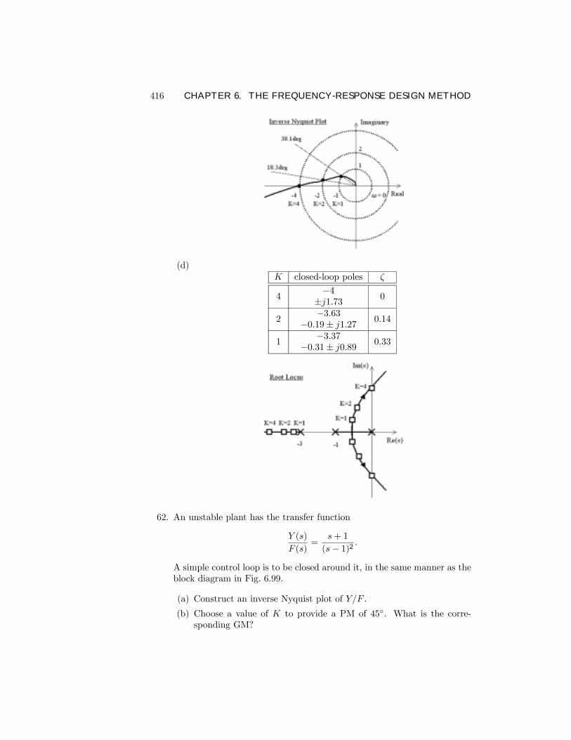
416 CHAPTER 6. THE FREQUENCY-RESPONSE DESIGN METHOD
(d)K closed-loop poles ζ
4−4
±j1.73 0
2−3.63
−0.19± j1.27 0.14
1−3.37
−0.31± j0.89 0.33
62. An unstable plant has the transfer function
Y (s)
F (s)=
s+ 1
(s− 1)2 .
A simple control loop is to be closed around it, in the same manner as theblock diagram in Fig. 6.99.
(a) Construct an inverse Nyquist plot of Y/F .
(b) Choose a value of K to provide a PM of 45. What is the corre-sponding GM?
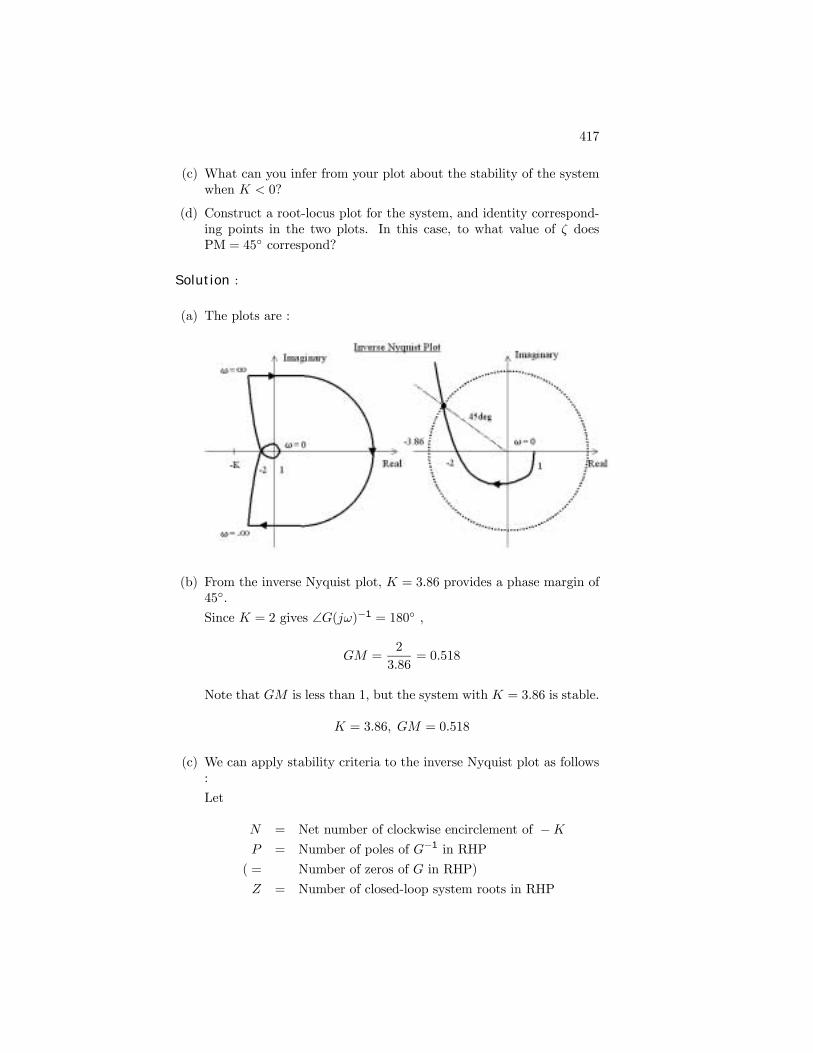
417
(c) What can you infer from your plot about the stability of the systemwhen K < 0?
(d) Construct a root-locus plot for the system, and identity correspond-ing points in the two plots. In this case, to what value of ζ doesPM = 45 correspond?
Solution :
(a) The plots are :
(b) From the inverse Nyquist plot, K = 3.86 provides a phase margin of45.Since K = 2 gives ∠G(jω)−1 = 180 ,
GM =2
3.86= 0.518
Note that GM is less than 1, but the system with K = 3.86 is stable.
K = 3.86, GM = 0.518
(c) We can apply stability criteria to the inverse Nyquist plot as follows:
Let
N = Net number of clockwise encirclement of −KP = Number of poles of G−1 in RHP
( = Number of zeros of G in RHP)
Z = Number of closed-loop system roots in RHP
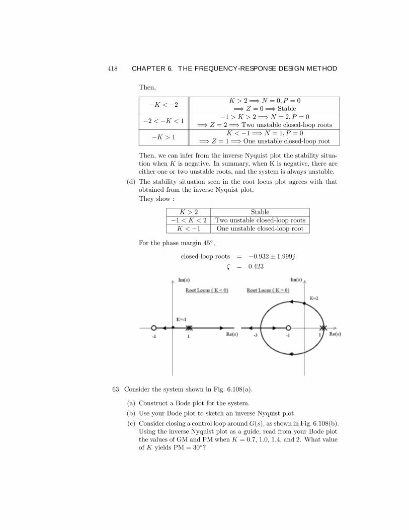
418 CHAPTER 6. THE FREQUENCY-RESPONSE DESIGN METHOD
Then,
−K < −2 K > 2 =⇒ N = 0, P = 0=⇒ Z = 0 =⇒ Stable
−2 < −K < 1−1 > K > 2 =⇒ N = 2, P = 0
=⇒ Z = 2 =⇒ Two unstable closed-loop roots
−K > 1K < −1 =⇒ N = 1, P = 0
=⇒ Z = 1 =⇒ One unstable closed-loop root
Then, we can infer from the inverse Nyquist plot the stability situa-tion when K is negative. In summary, when K is negative, there areeither one or two unstable roots, and the system is always unstable.
(d) The stability situation seen in the root locus plot agrees with thatobtained from the inverse Nyquist plot.
They show :
K > 2 Stable−1 < K < 2 Two unstable closed-loop rootsK < −1 One unstable closed-loop root
For the phase margin 45,
closed-loop roots = −0.932± 1.999jζ = 0.423
63. Consider the system shown in Fig. 6.108(a).
(a) Construct a Bode plot for the system.
(b) Use your Bode plot to sketch an inverse Nyquist plot.
(c) Consider closing a control loop aroundG(s), as shown in Fig. 6.108(b).Using the inverse Nyquist plot as a guide, read from your Bode plotthe values of GM and PM when K = 0.7, 1.0, 1.4, and 2. What valueof K yields PM = 30?
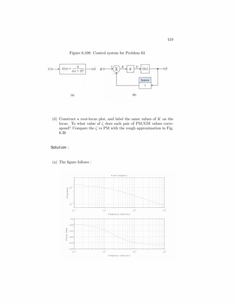
419
Figure 6.108: Control system for Problem 63
(d) Construct a root-locus plot, and label the same values of K on thelocus. To what value of ζ does each pair of PM/GM values corre-spond? Compare the ζ vs PM with the rough approximation in Fig.6.36
Solution :
(a) The Þgure follows :
10-1
100
101
102
10-5
100
Frequency (rad/sec)
Magnitude
B ode D iagram s
10-1
100
101
102
-300
-250
-200
-150
-100
-50
Frequency (rad/sec)
Phase (deg)
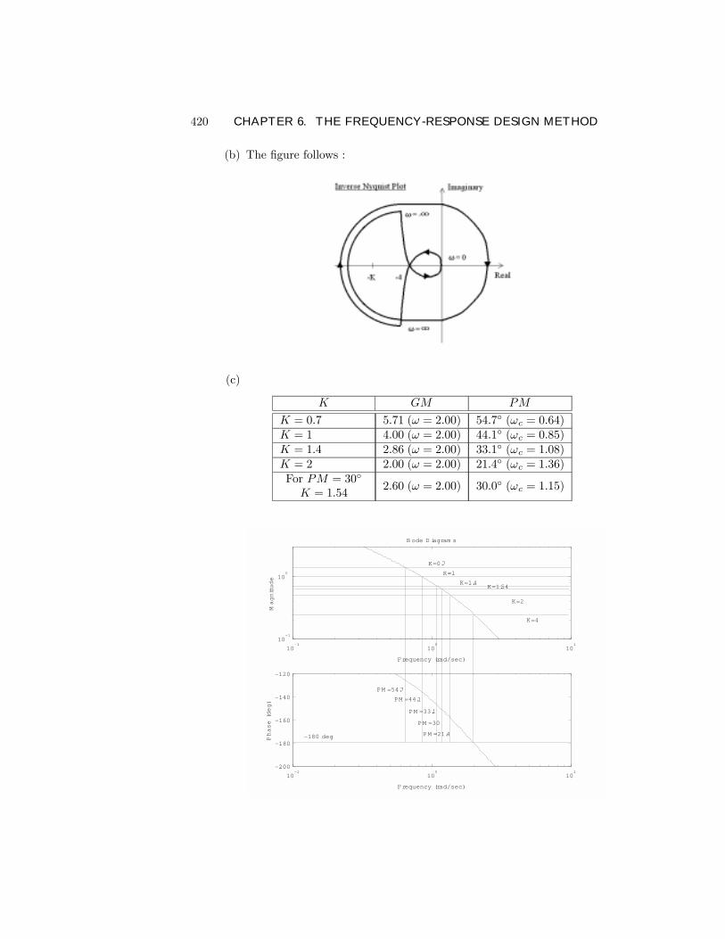
420 CHAPTER 6. THE FREQUENCY-RESPONSE DESIGN METHOD
(b) The Þgure follows :
(c)
K GM PM
K = 0.7 5.71 (ω = 2.00) 54.7 (ωc = 0.64)K = 1 4.00 (ω = 2.00) 44.1 (ωc = 0.85)K = 1.4 2.86 (ω = 2.00) 33.1 (ωc = 1.08)K = 2 2.00 (ω = 2.00) 21.4 (ωc = 1.36)For PM = 30
K = 1.542.60 (ω = 2.00) 30.0 (ωc = 1.15)
10-1
100
101
10-1
100
Frequency (rad/sec)
Magnitude
B ode D iagram s
10-1
100
101
-200
-180
-160
-140
-120
Frequency (rad/sec)
Phase (deg)
-180 deg
PM =54.7
PM =44.1
PM =33.1
PM =30
PM =21.4
K=0.7
K=1
K=1.4 K=1.54
K=2
K=4
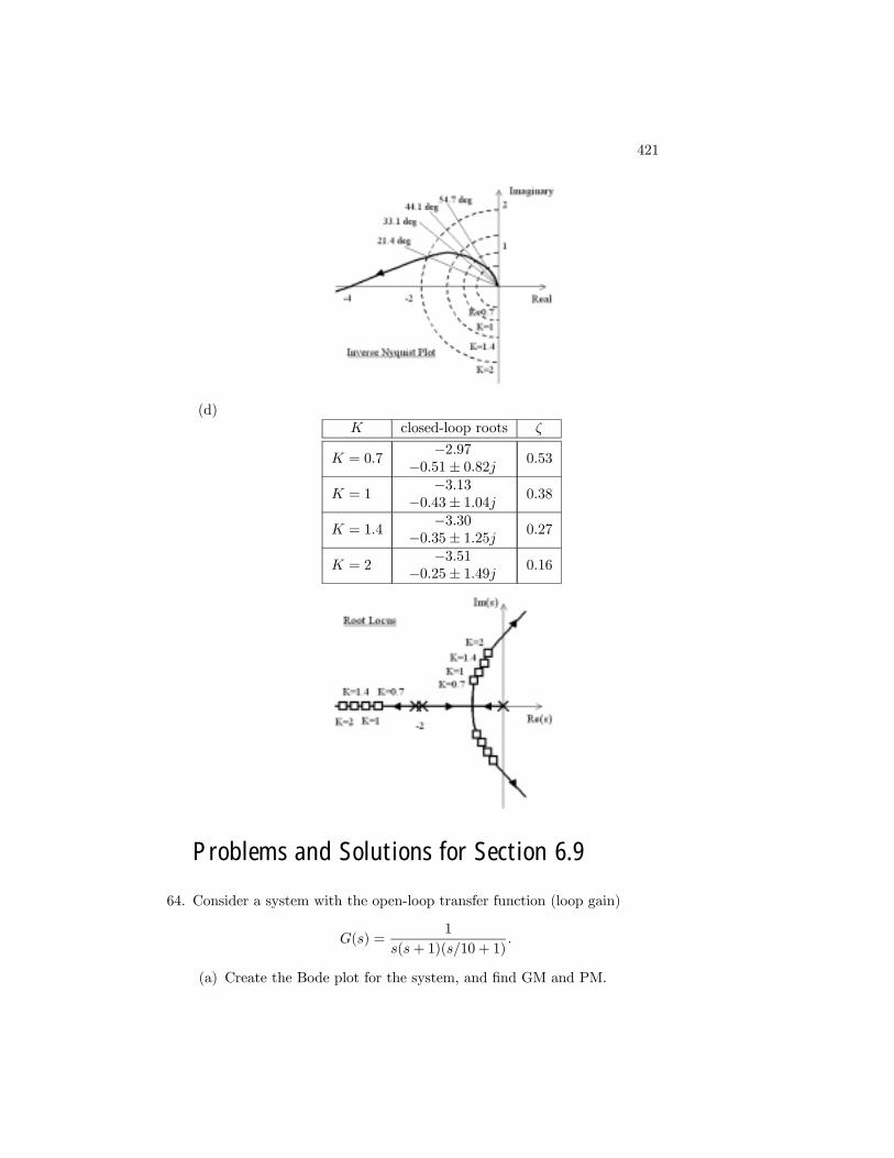
421
(d)K closed-loop roots ζ
K = 0.7−2.97
−0.51± 0.82j 0.53
K = 1−3.13
−0.43± 1.04j 0.38
K = 1.4−3.30
−0.35± 1.25j 0.27
K = 2−3.51
−0.25± 1.49j 0.16
Problems and Solutions for Section 6.9
64. Consider a system with the open-loop transfer function (loop gain)
G(s) =1
s(s+ 1)(s/10 + 1).
(a) Create the Bode plot for the system, and Þnd GM and PM.
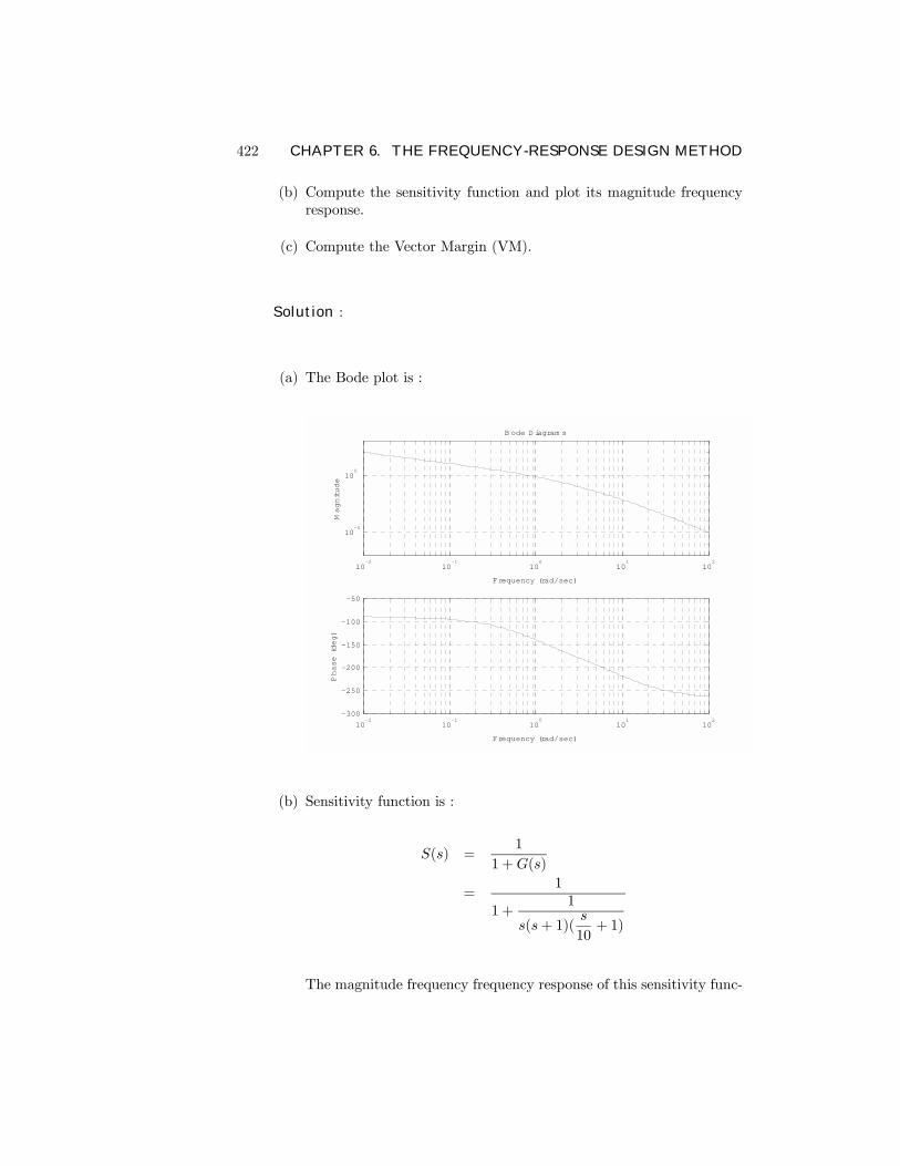
422 CHAPTER 6. THE FREQUENCY-RESPONSE DESIGN METHOD
(b) Compute the sensitivity function and plot its magnitude frequencyresponse.
(c) Compute the Vector Margin (VM).
Solution :
(a) The Bode plot is :
10-2
10-1
100
101
102
10-5
100
Frequency (rad/sec)
Magnitude
B ode D iagram s
10-2
10-1
100
101
102
-300
-250
-200
-150
-100
-50
Frequency (rad/sec)
Phase (deg)
(b) Sensitivity function is :
S(s) =1
1 +G(s)
=1
1 +1
s(s+ 1)(s
10+ 1)
The magnitude frequency frequency response of this sensitivity func-
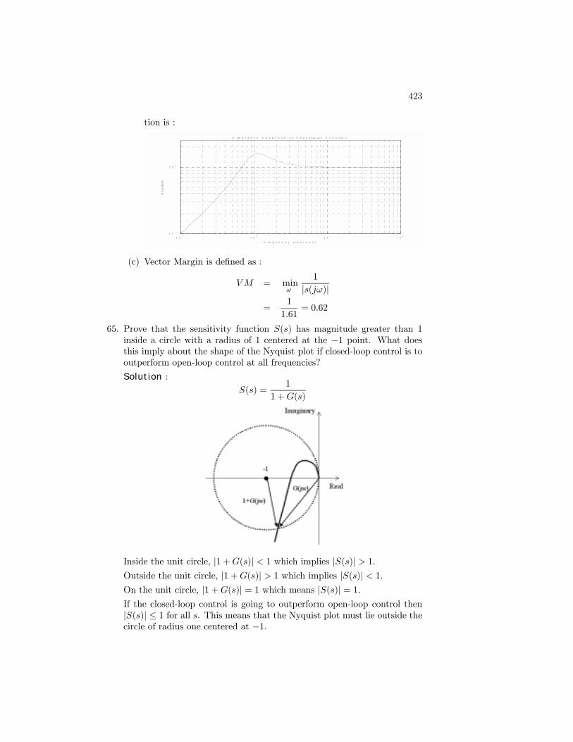
423
tion is :
1 0- 1
1 00
1 01
1 02
1 0- 1
1 00
F re q u e n c y (ra d / s e c )
Magnitude
F r e q u e n c y R e s p o n s e o f S e n s it iv ity F u n c tio n
(c) Vector Margin is deÞned as :
VM = minω
1
|s(jω)|=
1
1.61= 0.62
65. Prove that the sensitivity function S(s) has magnitude greater than 1inside a circle with a radius of 1 centered at the −1 point. What doesthis imply about the shape of the Nyquist plot if closed-loop control is tooutperform open-loop control at all frequencies?
Solution :
S(s) =1
1 +G(s)
Inside the unit circle, |1 +G(s)| < 1 which implies |S(s)| > 1.Outside the unit circle, |1 +G(s)| > 1 which implies |S(s)| < 1.On the unit circle, |1 +G(s)| = 1 which means |S(s)| = 1.If the closed-loop control is going to outperform open-loop control then|S(s)| ≤ 1 for all s. This means that the Nyquist plot must lie outside thecircle of radius one centered at −1.
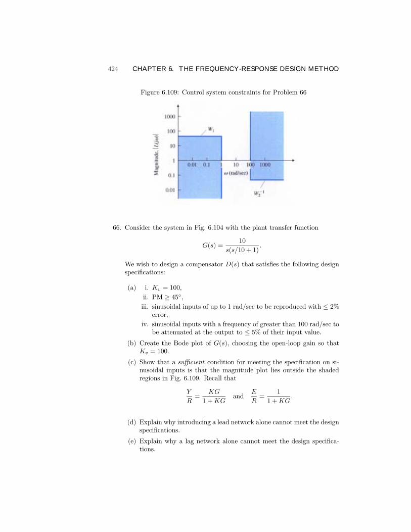
424 CHAPTER 6. THE FREQUENCY-RESPONSE DESIGN METHOD
Figure 6.109: Control system constraints for Problem 66
66. Consider the system in Fig. 6.104 with the plant transfer function
G(s) =10
s(s/10 + 1).
We wish to design a compensator D(s) that satisÞes the following designspeciÞcations:
(a) i. Kv = 100,
ii. PM ≥ 45,iii. sinusoidal inputs of up to 1 rad/sec to be reproduced with ≤ 2%
error,
iv. sinusoidal inputs with a frequency of greater than 100 rad/sec tobe attenuated at the output to ≤ 5% of their input value.
(b) Create the Bode plot of G(s), choosing the open-loop gain so thatKv = 100.
(c) Show that a sufficient condition for meeting the speciÞcation on si-nusoidal inputs is that the magnitude plot lies outside the shadedregions in Fig. 6.109. Recall that
Y
R=
KG
1 +KGand
E
R=
1
1 +KG.
(d) Explain why introducing a lead network alone cannot meet the designspeciÞcations.
(e) Explain why a lag network alone cannot meet the design speciÞca-tions.
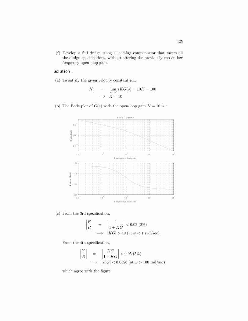
425
(f) Develop a full design using a lead-lag compensator that meets allthe design speciÞcations, without altering the previously chosen lowfrequency open-loop gain.
Solution :
(a) To satisfy the given velocity constant Kv,
Kv = lims→0
sKG(s) = 10K = 100
=⇒ K = 10
(b) The Bode plot of G(s) with the open-loop gain K = 10 is :
10-1
100
101
102
103
10-2
100
102
Frequency (rad/sec)
Magnitude
B ode D iagram s
10-1
100
101
102
103
-200
-160
-120
-80
Frequency (rad/sec)
Phase (deg)
(c) From the 3rd speciÞcation,¯E
R
¯=
¯1
1 +KG
¯< 0.02 (2%)
=⇒ |KG| > 49 (at ω < 1 rad/sec)
From the 4th speciÞcation,¯Y
R
¯=
¯KG
1 +KG
¯< 0.05 (5%)
=⇒ |KG| < 0.0526 (at ω > 100 rad/sec)
which agree with the Þgure.
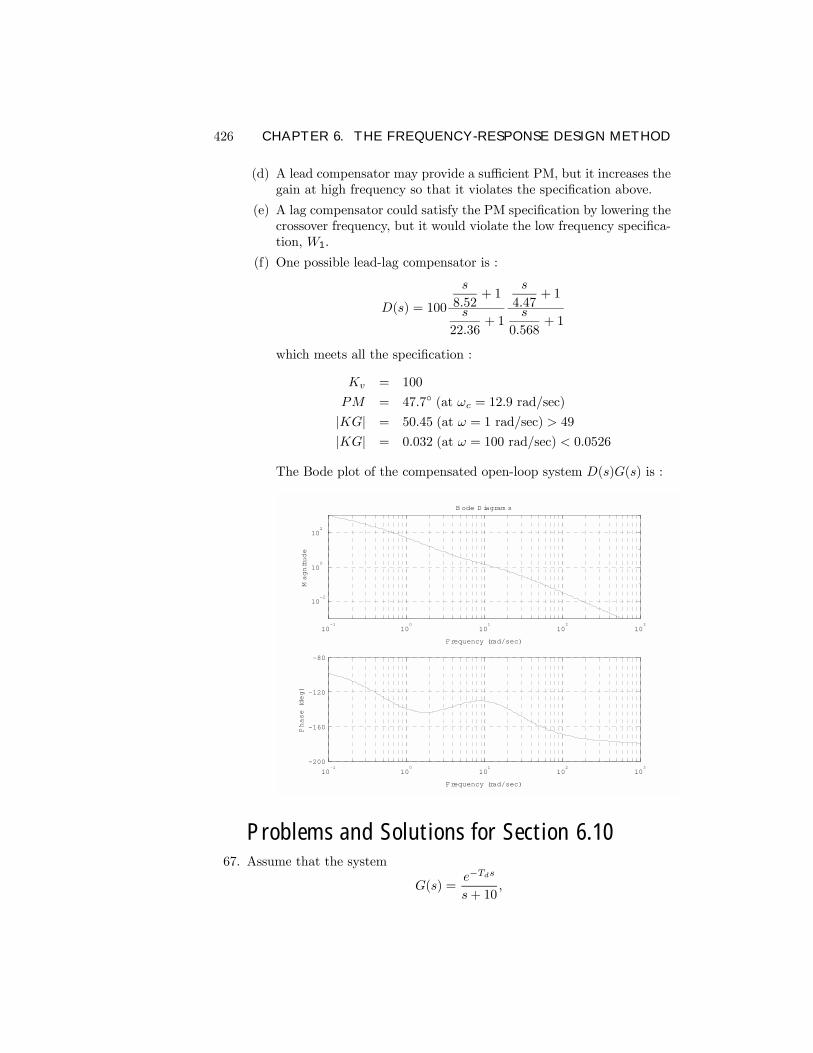
426 CHAPTER 6. THE FREQUENCY-RESPONSE DESIGN METHOD
(d) A lead compensator may provide a sufficient PM, but it increases thegain at high frequency so that it violates the speciÞcation above.
(e) A lag compensator could satisfy the PM speciÞcation by lowering thecrossover frequency, but it would violate the low frequency speciÞca-tion, W1.
(f) One possible lead-lag compensator is :
D(s) = 100
s
8.52+ 1
s
22.36+ 1
s
4.47+ 1
s
0.568+ 1
which meets all the speciÞcation :
Kv = 100
PM = 47.7 (at ωc = 12.9 rad/sec)|KG| = 50.45 (at ω = 1 rad/sec) > 49
|KG| = 0.032 (at ω = 100 rad/sec) < 0.0526
The Bode plot of the compensated open-loop system D(s)G(s) is :
10-1
100
101
102
103
10-2
100
102
Frequency (rad/sec)
Magnitude
B ode D iagram s
10-1
100
101
102
103
-200
-160
-120
-80
Frequency (rad/sec)
Phase (deg)
Problems and Solutions for Section 6.1067. Assume that the system
G(s) =e−Tds
s+ 10,
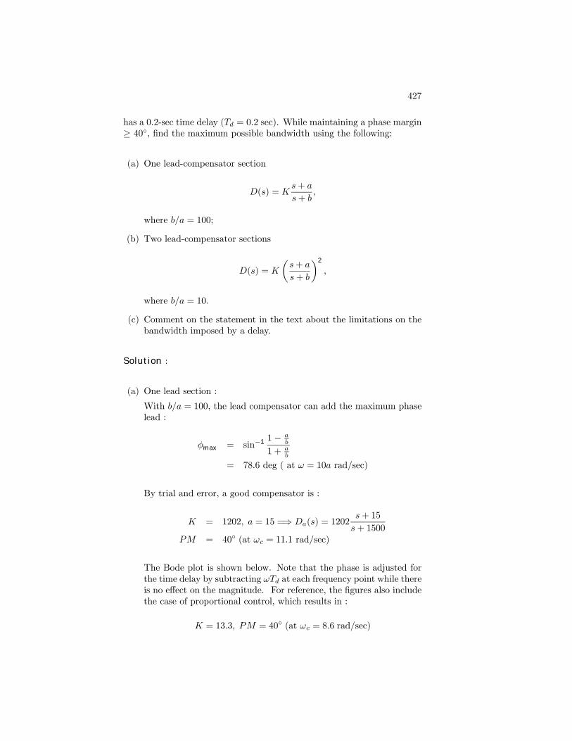
427
has a 0.2-sec time delay (Td = 0.2 sec). While maintaining a phase margin≥ 40, Þnd the maximum possible bandwidth using the following:
(a) One lead-compensator section
D(s) = Ks+ a
s+ b,
where b/a = 100;
(b) Two lead-compensator sections
D(s) = K
µs+ a
s+ b
¶2
,
where b/a = 10.
(c) Comment on the statement in the text about the limitations on thebandwidth imposed by a delay.
Solution :
(a) One lead section :
With b/a = 100, the lead compensator can add the maximum phaselead :
φmax = sin−1 1− ab
1 + ab
= 78.6 deg ( at ω = 10a rad/sec)
By trial and error, a good compensator is :
K = 1202, a = 15 =⇒ Da(s) = 1202s+ 15
s+ 1500PM = 40 (at ωc = 11.1 rad/sec)
The Bode plot is shown below. Note that the phase is adjusted forthe time delay by subtracting ωTd at each frequency point while thereis no effect on the magnitude. For reference, the Þgures also includethe case of proportional control, which results in :
K = 13.3, PM = 40 (at ωc = 8.6 rad/sec)
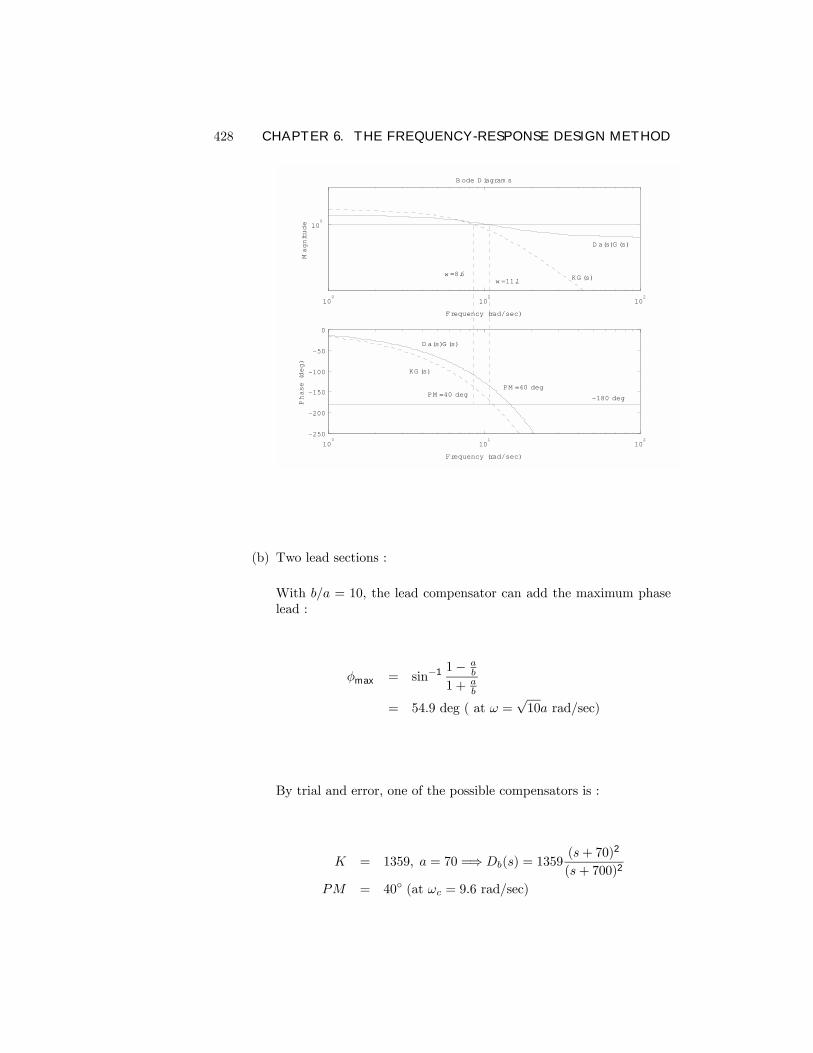
428 CHAPTER 6. THE FREQUENCY-RESPONSE DESIGN METHOD
100
101
102
100
Frequency (rad/sec)Magnitude
B ode D iagram s
100
101
102
-250
-200
-150
-100
-50
0
Frequency (rad/sec)
Phase (deg)
-180 deg
KG (s)
D a(s)G (s)
D a(s)G (s)
KG (s)
PM =40 deg PM =40 deg
w =11.1 w =8.6
(b) Two lead sections :
With b/a = 10, the lead compensator can add the maximum phaselead :
φmax = sin−1 1− ab
1 + ab
= 54.9 deg ( at ω =√10a rad/sec)
By trial and error, one of the possible compensators is :
K = 1359, a = 70 =⇒ Db(s) = 1359(s+ 70)2
(s+ 700)2
PM = 40 (at ωc = 9.6 rad/sec)
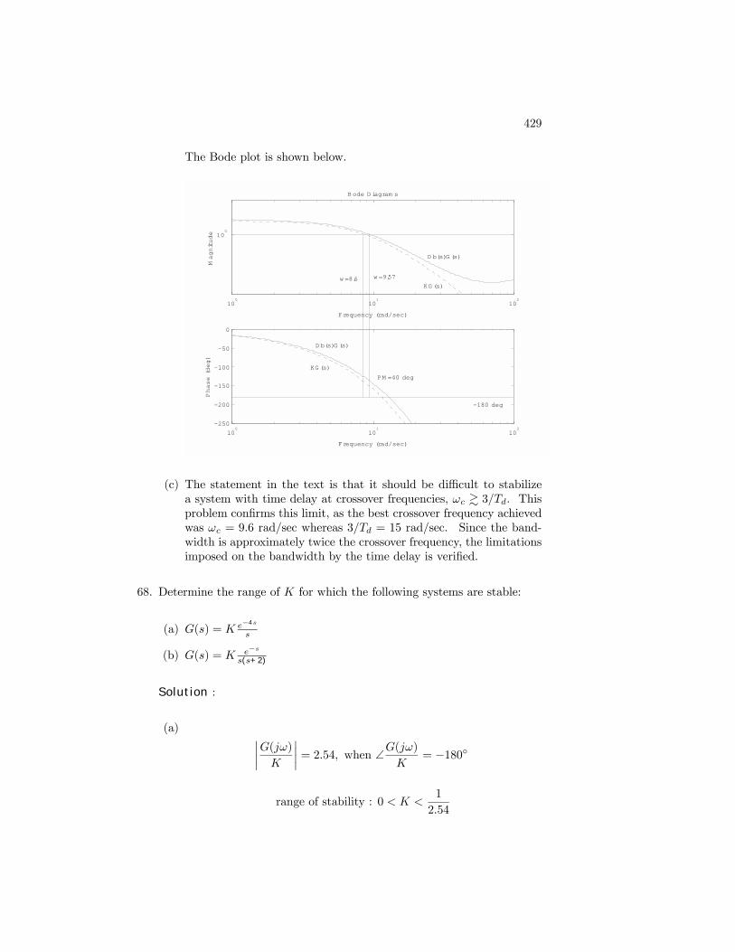
429
The Bode plot is shown below.
100
101
102
100
Frequency (rad/sec)
Magnitude
B ode D iagram s
100
101
102
-250
-200
-150
-100
-50
0
Frequency (rad/sec)
Phase (deg)
-180 deg
D b(s)G (s)
KG (s)
D b(s)G (s)
KG (s)
PM =40 deg
w =9.57 w =8.6
(c) The statement in the text is that it should be difficult to stabilizea system with time delay at crossover frequencies, ωc & 3/Td. Thisproblem conÞrms this limit, as the best crossover frequency achievedwas ωc = 9.6 rad/sec whereas 3/Td = 15 rad/sec. Since the band-width is approximately twice the crossover frequency, the limitationsimposed on the bandwidth by the time delay is veriÞed.
68. Determine the range of K for which the following systems are stable:
(a) G(s) = K e−4s
s
(b) G(s) = K e−ss(s+2)
Solution :
(a) ¯G(jω)
K
¯= 2.54, when ∠G(jω)
K= −180
range of stability : 0 < K <1
2.54
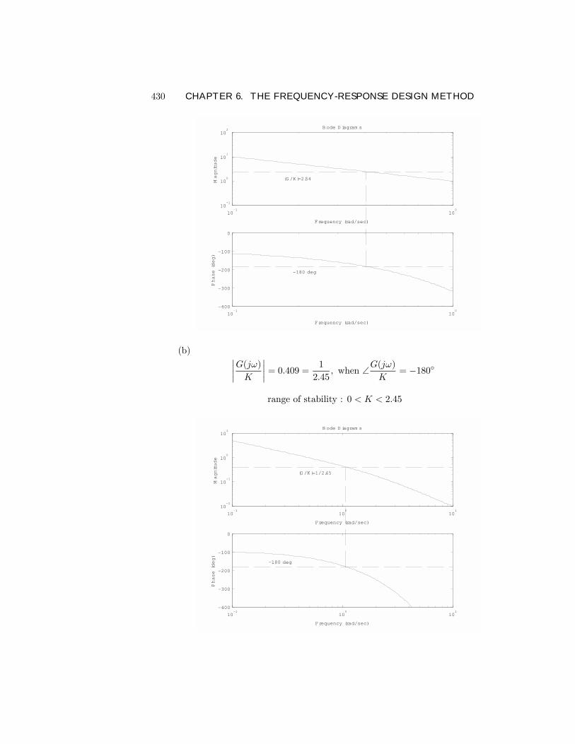
430 CHAPTER 6. THE FREQUENCY-RESPONSE DESIGN METHOD
10-1
100
10-1
100
101
102
Frequency (rad/sec)Magnitude
B ode D iagram s
10-1
100
-400
-300
-200
-100
0
Frequency (rad/sec)
Phase (deg)
-180 deg
|G /K|=2.54
(b) ¯G(jω)
K
¯= 0.409 =
1
2.45, when ∠G(jω)
K= −180
range of stability : 0 < K < 2.45
10-1
100
101
10-2
10-1
100
101
Frequency (rad/sec)
Magnitude
B ode D iagram s
10-1
100
101
-400
-300
-200
-100
0
Frequency (rad/sec)
Phase (deg)
-180 deg
|G /K|=1/2.45
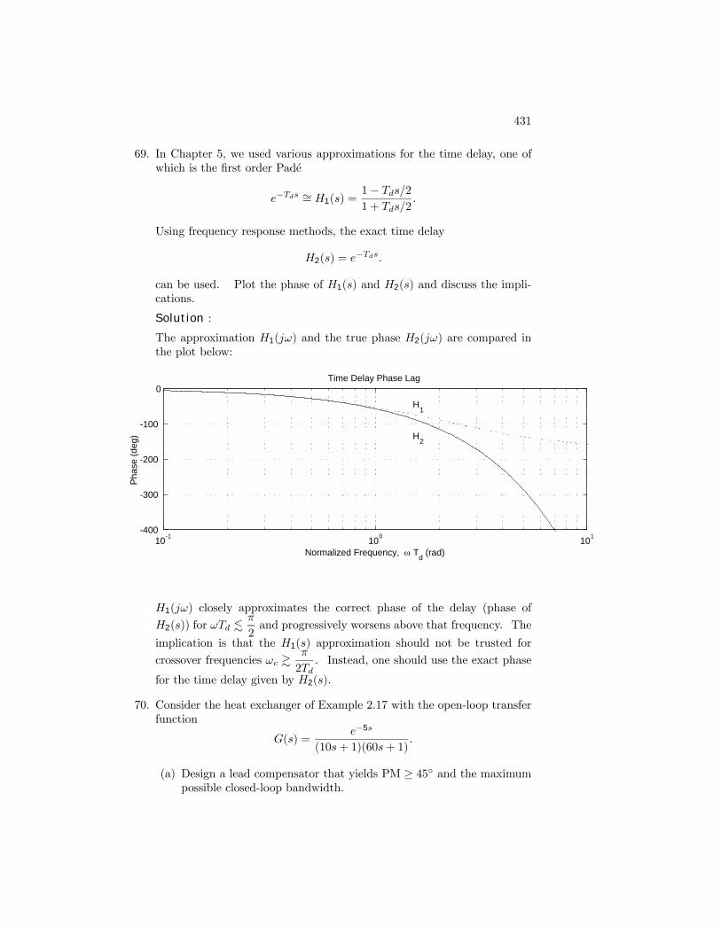
431
69. In Chapter 5, we used various approximations for the time delay, one ofwhich is the Þrst order Pade
e−Tds ∼= H1(s) =1− Tds/21 + Tds/2
.
Using frequency response methods, the exact time delay
H2(s) = e−Tds.
can be used. Plot the phase of H1(s) and H2(s) and discuss the impli-cations.
Solution :
The approximation H1(jω) and the true phase H2(jω) are compared inthe plot below:
10-1 100 101-400
-300
-200
-100
0
Normalized Frequency, Td (rad)
Phas
e (d
eg)
Time Delay Phase Lag
H1
H2
H1(jω) closely approximates the correct phase of the delay (phase of
H2(s)) for ωTd .π
2and progressively worsens above that frequency. The
implication is that the H1(s) approximation should not be trusted for
crossover frequencies ωc &π
2Td. Instead, one should use the exact phase
for the time delay given by H2(s).
70. Consider the heat exchanger of Example 2.17 with the open-loop transferfunction
G(s) =e−5s
(10s+ 1)(60s+ 1).
(a) Design a lead compensator that yields PM ≥ 45 and the maximumpossible closed-loop bandwidth.
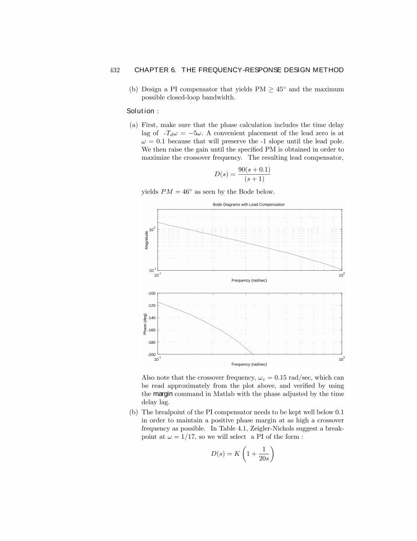
432 CHAPTER 6. THE FREQUENCY-RESPONSE DESIGN METHOD
(b) Design a PI compensator that yields PM ≥ 45 and the maximumpossible closed-loop bandwidth.
Solution :
(a) First, make sure that the phase calculation includes the time delaylag of -Tdω = −5ω. A convenient placement of the lead zero is atω = 0.1 because that will preserve the -1 slope until the lead pole.We then raise the gain until the speciÞed PM is obtained in order tomaximize the crossover frequency. The resulting lead compensator,
D(s) =90(s+ 0.1)
(s+ 1)
yields PM = 46 as seen by the Bode below.
10-1 10010-1
100
Frequency (rad/sec)
Mag
nitu
de
Bode Diagrams with Lead Compensation
10-1 100-200
-180
-160
-140
-120
-100
Frequency (rad/sec)
Phas
e (d
eg)
Also note that the crossover frequency, ωc = 0.15 rad/sec, which canbe read approximately from the plot above, and veriÞed by usingthe margin command in Matlab with the phase adjusted by the timedelay lag.
(b) The brealpoint of the PI compensator needs to be kept well below 0.1in order to maintain a positive phase margin at as high a crossoverfrequency as possible. In Table 4.1, Zeigler-Nichols suggest a break-point at ω = 1/17, so we will select a PI of the form :
D(s) = K
µ1 +
1
20s
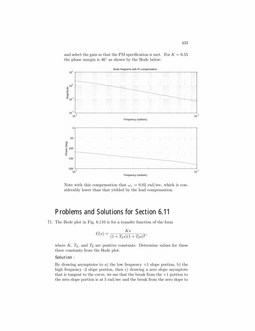
433
and select the gain so that the PM speciÞcation is met. ForK = 0.55the phase margin is 46 as shown by the Bode below:
10-2 10-110-2
10-1
100
101
Frequency (rad/sec)
Mag
nitu
deBode Diagrams with PI compensation
10-2 10-1-200
-150
-100
-50
0
Frequency (rad/sec)
Phas
e (d
eg)
Note with this compensation that ωc = 0.02 rad/sec, which is con-siderably lower than that yielded by the lead compensation.
Problems and Solutions for Section 6.11
71. The Bode plot in Fig. 6.110 is for a transfer function of the form
G(s) =Ks
(1 + T1s)(1 + T2s)2,
where K, T1, and T2 are positive constants. Determine values for thesethree constants from the Bode plot.
Solution :
By drawing asymptotes to a) the low frequency +1 slope portion, b) thehigh frequency -2 slope portion, then c) drawing a zero slope asymptotethat is tangent to the curve, we see that the break from the +1 portion tothe zero slope portion is at 5 rad/sec and the break from the zero slope to
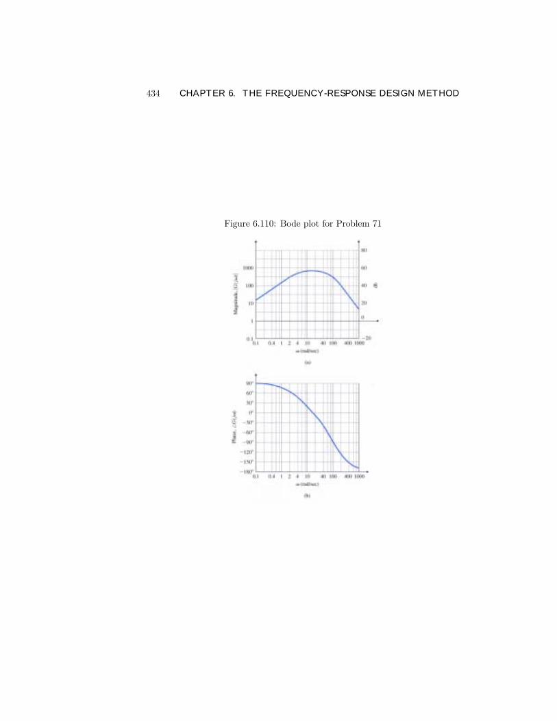
434 CHAPTER 6. THE FREQUENCY-RESPONSE DESIGN METHOD
Figure 6.110: Bode plot for Problem 71
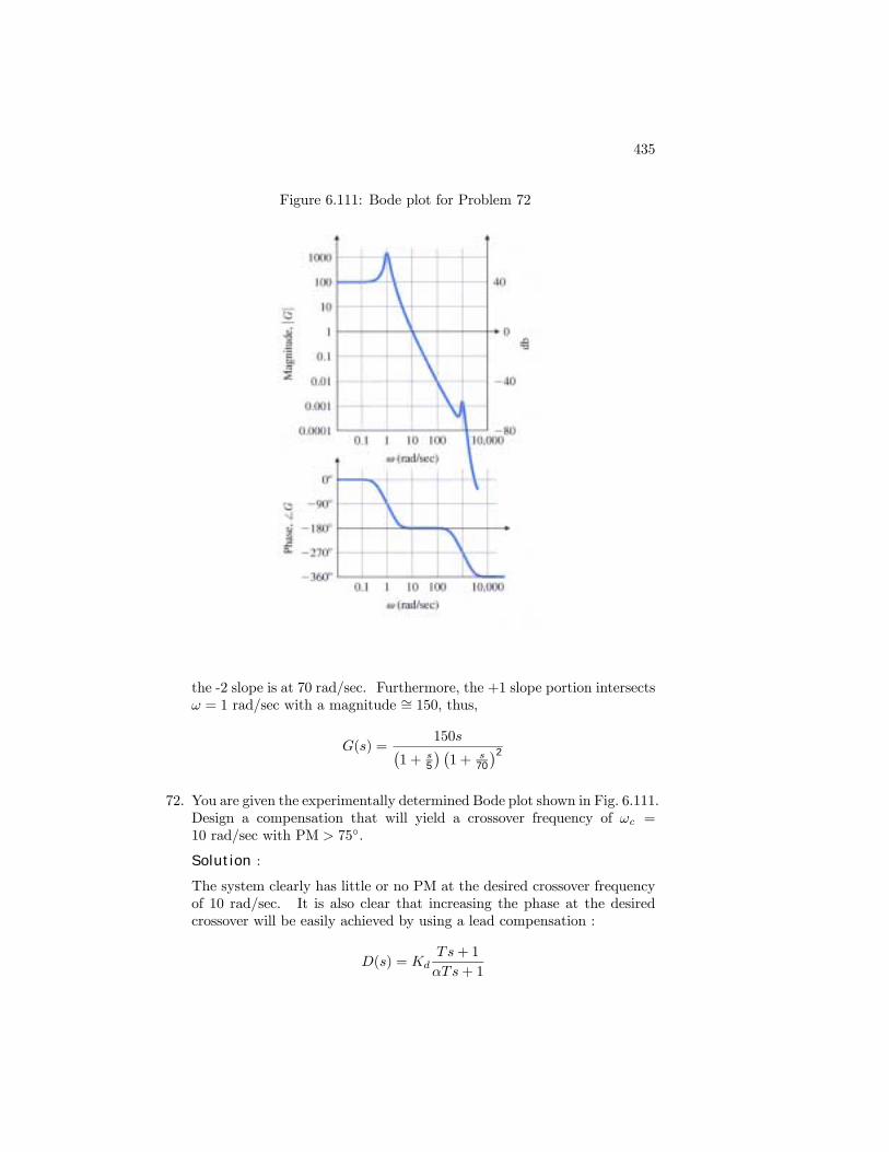
435
Figure 6.111: Bode plot for Problem 72
the -2 slope is at 70 rad/sec. Furthermore, the +1 slope portion intersectsω = 1 rad/sec with a magnitude ∼= 150, thus,
G(s) =150s¡
1 + s5
¢ ¡1 + s
70
¢2
72. You are given the experimentally determined Bode plot shown in Fig. 6.111.Design a compensation that will yield a crossover frequency of ωc =10 rad/sec with PM > 75.
Solution :
The system clearly has little or no PM at the desired crossover frequencyof 10 rad/sec. It is also clear that increasing the phase at the desiredcrossover will be easily achieved by using a lead compensation :
D(s) = KdTs+ 1
αTs+ 1
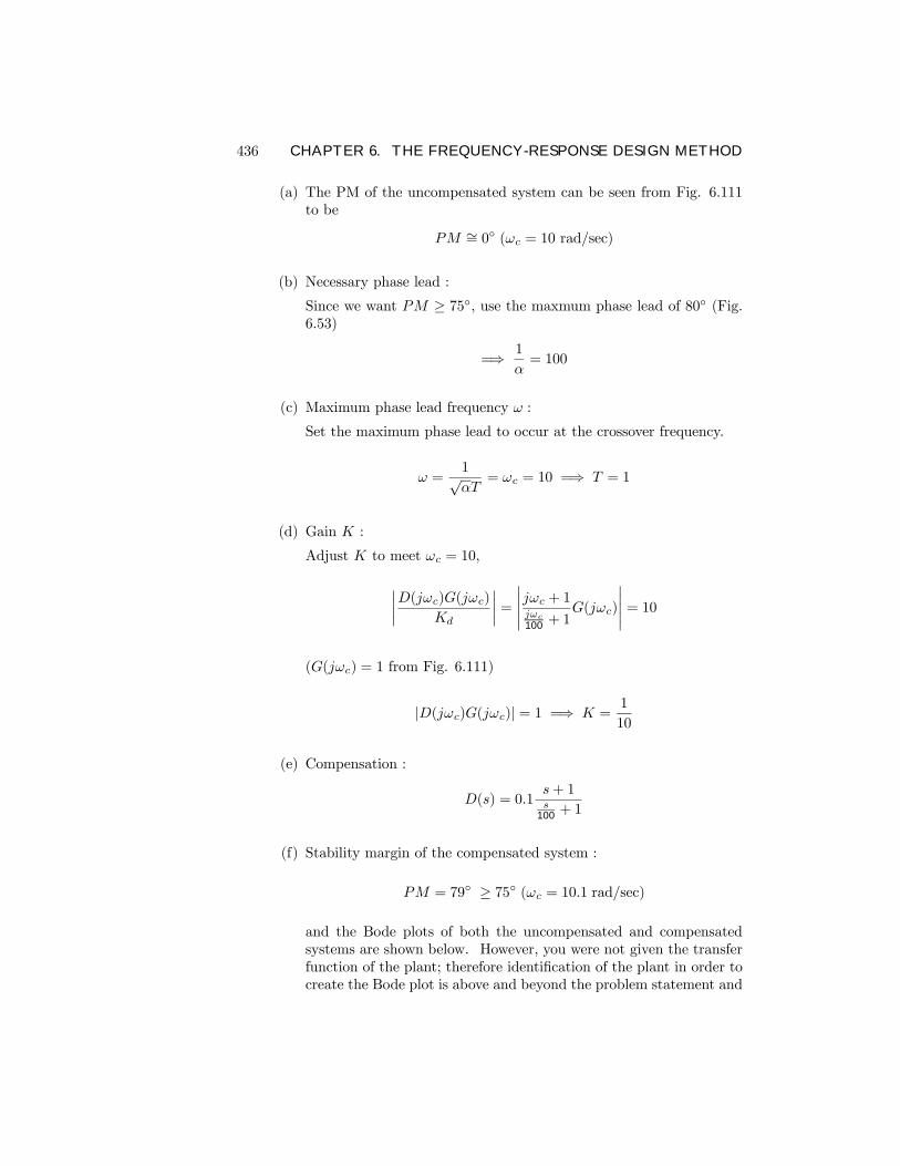
436 CHAPTER 6. THE FREQUENCY-RESPONSE DESIGN METHOD
(a) The PM of the uncompensated system can be seen from Fig. 6.111to be
PM ∼= 0 (ωc = 10 rad/sec)
(b) Necessary phase lead :
Since we want PM ≥ 75, use the maxmum phase lead of 80 (Fig.6.53)
=⇒ 1
α= 100
(c) Maximum phase lead frequency ω :
Set the maximum phase lead to occur at the crossover frequency.
ω =1√αT
= ωc = 10 =⇒ T = 1
(d) Gain K :
Adjust K to meet ωc = 10,
¯D(jωc)G(jωc)
Kd
¯=
¯¯jωc + 1jωc
100 + 1G(jωc)
¯¯ = 10
(G(jωc) = 1 from Fig. 6.111)
|D(jωc)G(jωc)| = 1 =⇒ K =1
10
(e) Compensation :
D(s) = 0.1s+ 1s
100 + 1
(f) Stability margin of the compensated system :
PM = 79 ≥ 75 (ωc = 10.1 rad/sec)
and the Bode plots of both the uncompensated and compensatedsystems are shown below. However, you were not given the transferfunction of the plant; therefore identiÞcation of the plant in order tocreate the Bode plot is above and beyond the problem statement and
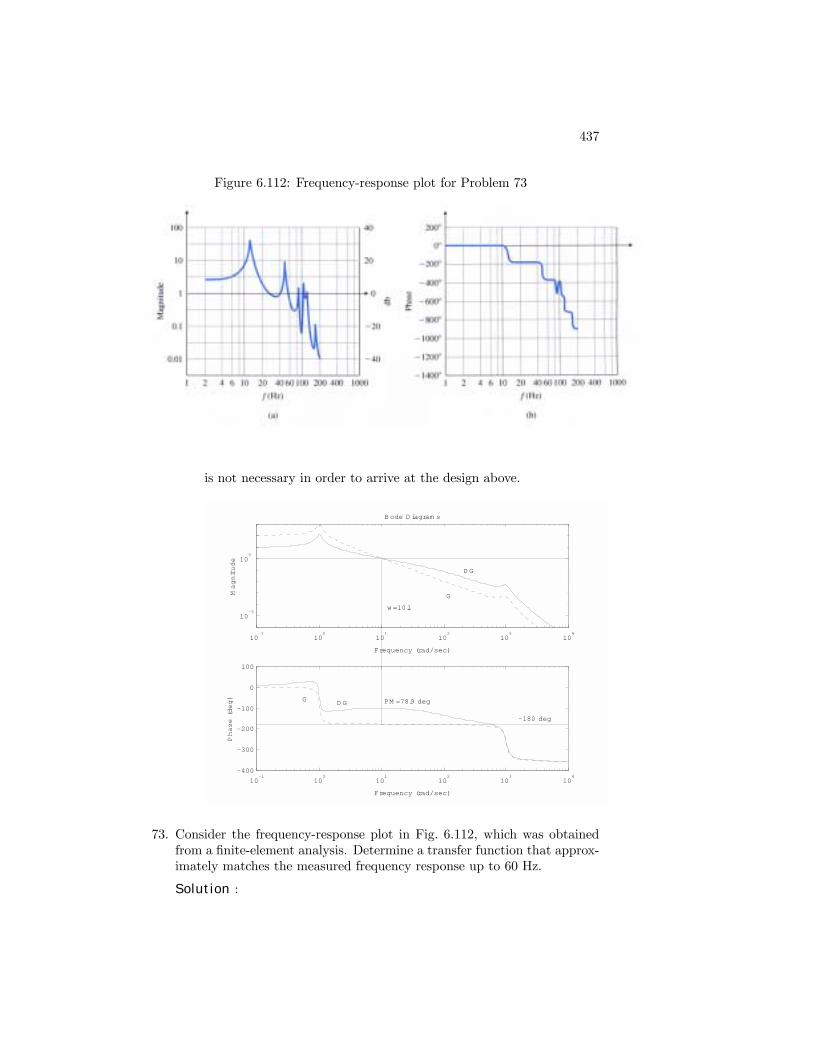
437
Figure 6.112: Frequency-response plot for Problem 73
is not necessary in order to arrive at the design above.
10-1
100
101
102
103
104
10-5
100
Frequency (rad/sec)
Magnitude
B ode D iagram s
10-1
100
101
102
103
104
-400
-300
-200
-100
0
100
Frequency (rad/sec)
Phase (deg)
w =10.1
-180 deg
PM =78.9 deg
D G
G
D G G
73. Consider the frequency-response plot in Fig. 6.112, which was obtainedfrom a Þnite-element analysis. Determine a transfer function that approx-imately matches the measured frequency response up to 60 Hz.
Solution :
438 CHAPTER 6. THE FREQUENCY-RESPONSE DESIGN METHOD
Considering only that portion of the Bode below ω = 60 Hz, we seetwo resonant peaks at ω = 12 Hz and ω = 50 Hz or ω = 75 rad/sec and ω =315 rad/sec. The phase curves conÞrm that there are two lightly dampedsecond order terms in the denominator at each of these two frequenciesbecause the phase decreases sharply by 180o at these frequencies. Twolightly damped second order terms in the denominator will also producethe peaks seen in the magnitude plot. The zero slope of the magnitudeand zero phase at low frequencies both indicate that it is a Type 0 system.Therefore, the form of the transfer function is
G(s) =K
( s2
ω21+ 2ζ1s
ω1+ 1)( s
2
ω22+ 2ζ2s
ω2+ 1)
where we have already determined that ω1 = 75 rad/sec and ω2 = 315rad/sec. By sketching in the zero slope low frequency portion of theasymptotes, we see that the Þrst resonant peak is approximately a factorof 20 above the asymptote. Resonant peaks are a factor of 1
2ζ above
the asympotes; therefore, 12ζ1
= 20 and ζ1 = 1/40 = 0.025. By carefully
drawing the -2 slope asymptote to intersect the zero slope asymptote atω1 = 12 Hz, we see that the second resonant peak is a factor of 50 above itsasymptote. Therefore, ζ2 = 1/100 = 0.01. The zero slope low frequencyasmptote has a magnitude of approximately 2.5. Filling in all the valuesproduces the transfer function,
G(s) =2.5
( s2
752 +0.05s
75 + 1)( s2
3152 +0.02s315 + 1)
74. The frequency response data shown in Table 6.1 were taken from a DCmotor that is to be used in a position control system. Assume that themotor is linear and minimum-phase.
(a) Estimate G(s), the transfer function of the system.
(b) Design a series compensator for the motor so that the closed-loopsystem meets the following speciÞcations:
i. The steady-state error to a unit ramp input is less than 0.01.
ii. PM ≥ = 45.
Solution :
(a) By plotting the points in the table, we see that the slope at lowfrequencies (< 1 rad/sec) is -1 and the slope at very high frequencies(>100 rad/sec) is -3. It is also apparent that the slope in the vicinityof 10 rad/sec is -2. Since there are no resonant peaks, the most likelytransfer function has two Þrst order breaks with one free power of sin the denominator in order to match the -1 slope at low frequencies.
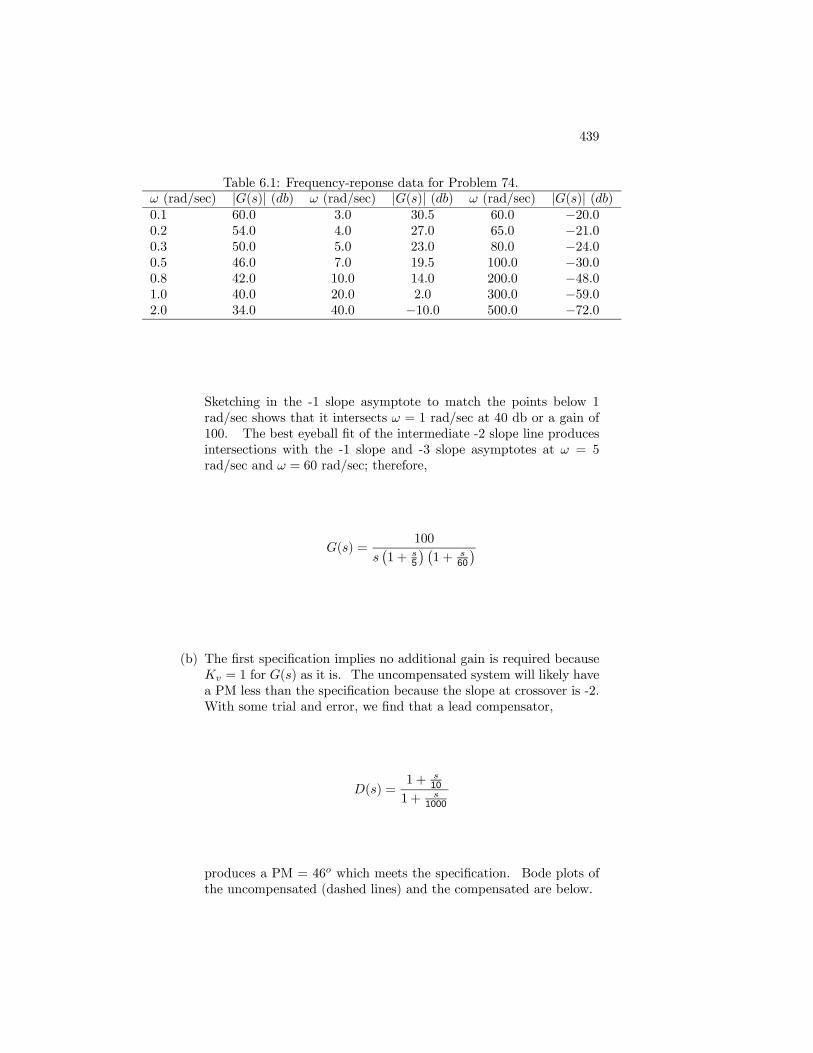
439
Table 6.1: Frequency-reponse data for Problem 74.ω (rad/sec) |G(s)| (db) ω (rad/sec) |G(s)| (db) ω (rad/sec) |G(s)| (db)0.1 60.0 3.0 30.5 60.0 −20.00.2 54.0 4.0 27.0 65.0 −21.00.3 50.0 5.0 23.0 80.0 −24.00.5 46.0 7.0 19.5 100.0 −30.00.8 42.0 10.0 14.0 200.0 −48.01.0 40.0 20.0 2.0 300.0 −59.02.0 34.0 40.0 −10.0 500.0 −72.0
Sketching in the -1 slope asymptote to match the points below 1rad/sec shows that it intersects ω = 1 rad/sec at 40 db or a gain of100. The best eyeball Þt of the intermediate -2 slope line producesintersections with the -1 slope and -3 slope asymptotes at ω = 5rad/sec and ω = 60 rad/sec; therefore,
G(s) =100
s¡1 + s
5
¢ ¡1 + s
60
¢
(b) The Þrst speciÞcation implies no additional gain is required becauseKv = 1 for G(s) as it is. The uncompensated system will likely havea PM less than the speciÞcation because the slope at crossover is -2.With some trial and error, we Þnd that a lead compensator,
D(s) =1 + s
10
1 + s1000
produces a PM = 46o which meets the speciÞcation. Bode plots ofthe uncompensated (dashed lines) and the compensated are below.
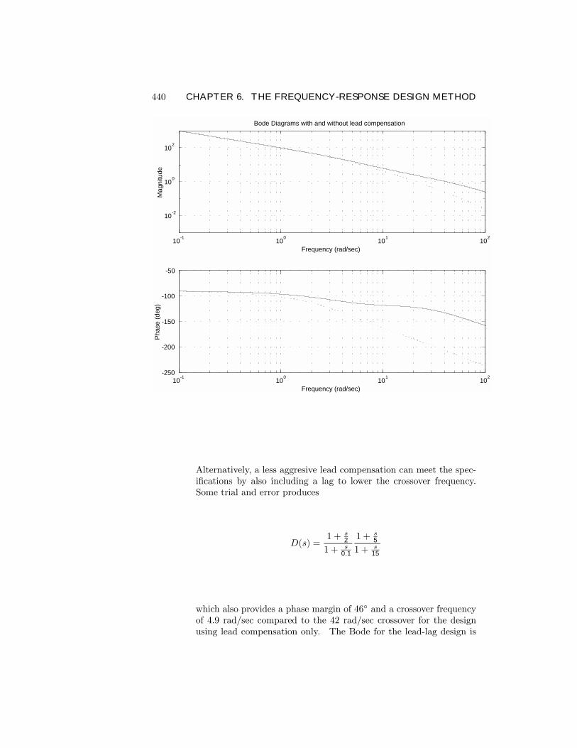
440 CHAPTER 6. THE FREQUENCY-RESPONSE DESIGN METHOD
10-1 100 101 102
10-2
100
102
Frequency (rad/sec)
Mag
nitu
de
Bode Diagrams with and without lead compensation
10-1 100 101 102-250
-200
-150
-100
-50
Frequency (rad/sec)
Phas
e (d
eg)
Alternatively, a less aggresive lead compensation can meet the spec-iÞcations by also including a lag to lower the crossover frequency.Some trial and error produces
D(s) =1 + s
2
1 + s0.1
1 + s5
1 + s15
which also provides a phase margin of 46 and a crossover frequencyof 4.9 rad/sec compared to the 42 rad/sec crossover for the designusing lead compensation only. The Bode for the lead-lag design is
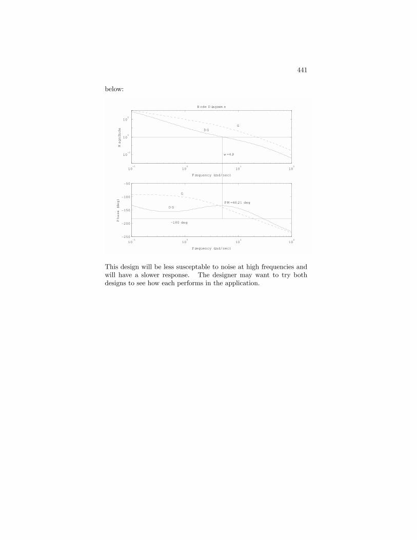
441
below:
10-1
100
101
102
10-2
100
102
Frequency (rad/sec)
Magnitude
B ode D iagram s
10-1
100
101
102
-250
-200
-150
-100
-50
Frequency (rad/sec)
Phase (deg)
G D G
G
D G
w =4.9
-180 deg
PM =46.21 deg
This design will be less susceptable to noise at high frequencies andwill have a slower response. The designer may want to try bothdesigns to see how each performs in the application.
Top Related