Supporting Information Multitude NMR Studies of α-Synuclein Familial Mutants: Probing Their Differential Aggregation Propensities Dipita Bhattacharyya,[a] Rakesh Kumar,[b] Surabhi Mehra,[b] Anirban Ghosh,[a] Samir K. Maji,*[b] Anirban Bhunia,*[a]

[a]Department of Biophysics, Bose Institute, P-1/12 CIT Scheme VII (M), Kolkata 700054, India [b]Department of Biosciences and Bioengineering, Indian Institute of Technology Bombay, Mumbai 400076 India

Corresponding Authors

Dr. Anirban Bhunia E-mail: bhunia@jcbose.ac.in or anirbanbhunia@gmail.com Dr. Samir K. Maji E-mail: samirmaji@iitb.ac.in

Electronic Supplementary Material (ESI) for ChemComm.This journal is © The Royal Society of Chemistry 2018

 

Abstract: Abstract: Familial mutations in α-synuclein affect the immediate chemical environment of the protein’s backbone, changing its aggregation kinetics, forming diverse structural and functional intermediates. This study, concerning two oppositely aggregating mutants A30P and E46K, reveals completely diverse conformational landscape for each, thus providing atomistic insights into differences in their aggregation dynamics.

 

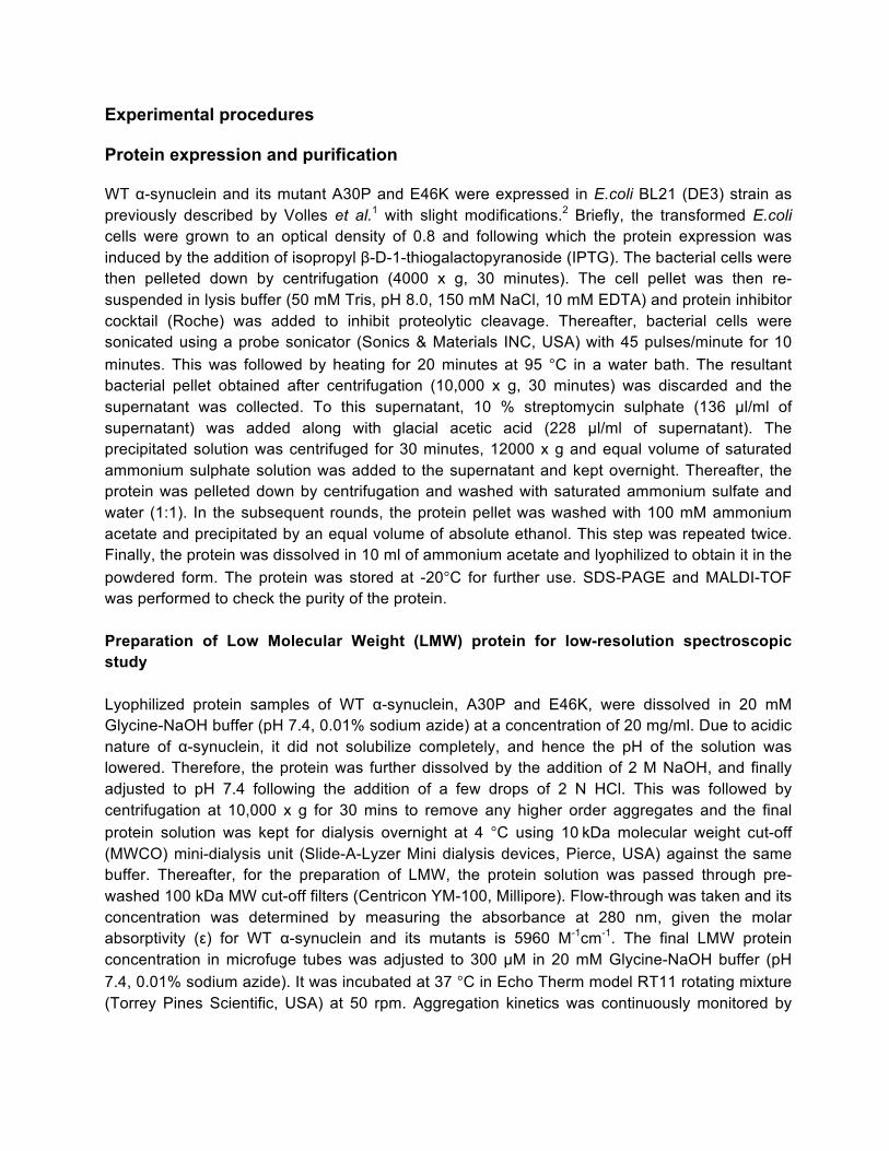
Experimental procedures Protein expression and purification WT α-synuclein and its mutant A30P and E46K were expressed in E.coli BL21 (DE3) strain as previously described by Volles et al.1 with slight modifications.2 Briefly, the transformed E.coli cells were grown to an optical density of 0.8 and following which the protein expression was induced by the addition of isopropyl β-D-1-thiogalactopyranoside (IPTG). The bacterial cells were then pelleted down by centrifugation (4000 x g, 30 minutes). The cell pellet was then re-suspended in lysis buffer (50 mM Tris, pH 8.0, 150 mM NaCl, 10 mM EDTA) and protein inhibitor cocktail (Roche) was added to inhibit proteolytic cleavage. Thereafter, bacterial cells were sonicated using a probe sonicator (Sonics & Materials INC, USA) with 45 pulses/minute for 10 minutes. This was followed by heating for 20 minutes at 95 °C in a water bath. The resultant bacterial pellet obtained after centrifugation (10,000 x g, 30 minutes) was discarded and the supernatant was collected. To this supernatant, 10 % streptomycin sulphate (136 µl/ml of supernatant) was added along with glacial acetic acid (228 µl/ml of supernatant). The precipitated solution was centrifuged for 30 minutes, 12000 x g and equal volume of saturated ammonium sulphate solution was added to the supernatant and kept overnight. Thereafter, the protein was pelleted down by centrifugation and washed with saturated ammonium sulfate and water (1:1). In the subsequent rounds, the protein pellet was washed with 100 mM ammonium acetate and precipitated by an equal volume of absolute ethanol. This step was repeated twice. Finally, the protein was dissolved in 10 ml of ammonium acetate and lyophilized to obtain it in the powdered form. The protein was stored at -20°C for further use. SDS-PAGE and MALDI-TOF was performed to check the purity of the protein. Preparation of Low Molecular Weight (LMW) protein for low-resolution spectroscopic study Lyophilized protein samples of WT α-synuclein, A30P and E46K, were dissolved in 20 mM Glycine-NaOH buffer (pH 7.4, 0.01% sodium azide) at a concentration of 20 mg/ml. Due to acidic nature of α-synuclein, it did not solubilize completely, and hence the pH of the solution was lowered. Therefore, the protein was further dissolved by the addition of 2 M NaOH, and finally adjusted to pH 7.4 following the addition of a few drops of 2 N HCl. This was followed by centrifugation at 10,000 x g for 30 mins to remove any higher order aggregates and the final protein solution was kept for dialysis overnight at 4 °C using 10  kDa molecular weight cut-off (MWCO) mini-dialysis unit (Slide-A-Lyzer Mini dialysis devices, Pierce, USA) against the same buffer. Thereafter, for the preparation of LMW, the protein solution was passed through pre-washed 100 kDa MW cut-off filters (Centricon YM-100, Millipore). Flow-through was taken and its concentration was determined by measuring the absorbance at 280 nm, given the molar absorptivity (ε) for WT α-synuclein and its mutants is 5960 M-1cm-1. The final LMW protein concentration in microfuge tubes was adjusted to 300 µΜ in 20 mM Glycine-NaOH buffer (pH 7.4, 0.01% sodium azide). It was incubated at 37 °C in Echo Therm model RT11 rotating mixture (Torrey Pines Scientific, USA) at 50 rpm. Aggregation kinetics was continuously monitored by

 

measuring time dependent secondary structural changes using circular dichroism (CD) spectroscopy and fibril formation by ThT fluorescence. Thioflavin T (ThT) Fluorescence assay Thioflavin T (ThT) has been effectively used to probe the presence of cross-β-sheet structures in amyloids.3 Aggregation kinetics for WT and mutants was carried out at 300 µM protein concentration. To measure ThT fluorescence, 5 µl samples were aliquoted from the main reaction sample volume and diluted to 200 µl in 20 mM Glycine-NaOH buffer (pH 7.4, 0.01% sodium azide) to make the final concentration of 7.5 µM. Thereafter, 2 µl of 1 mM ThT prepared in Tris-HCl buffer (pH 8.0, 0.01% Sodium azide) was added to the diluted protein sample. This was followed by immediate fluorescence measurement with an excitation wavelength of 450 nm, emission range 460-500 nm and slit width for both excitation and emission of 5 nm using the Horiba-JobinYvon (Fluomax4) instrument. ThT fluorescence intensity was monitored at 480 nm and at different time intervals for each of the three variants and plotted to fit in a sigmoidal curve. The lag time was calculated using the following equation (eq. 1), as published previously4: y = y0 + (ymax – y0 )/ (1+ e-(k(t-t

1/2)) ……………………………………………………………..eq. 1

where y is the ThT fluorescence at a particular time point, ymax is the maximum ThT fluorescence and y0 is the ThT fluorescence at t0 and tlag was defined as tlag = t½- 2/k. The nucleation rate (k) (h-1) was calculated as inverse of the lag time determined (Table S1). For calculating elongation rate, the ThT fluorescence data from the beginning of the elongation phase till the end of elongation phase was plotted and fitted linearly. The slope provides the elongation rate. Three independent experiments were performed throughout. Circular Dichroism (CD) Spectroscopy To record the CD spectra, 5 µl of protein sample from the main reaction tube (300 µM) was diluted to 200 µl of 20 mM Glycine-NaOH buffer (pH 7.4, 0.01% sodium azide) making the final concentration of protein to about 7.5 µΜ. The diluted sample was taken in a thoroughly washed quartz cell (Hellma, Forest Hills, NY) with path length of 0.1 cm and the spectra were obtained within the wavelength range of 198-260 nm at 25 °C by CD instrument (JASCO-810). For each spectrum, three readings were taken (i.e. three accumulations) and the average was considered. Smoothing and buffer subtraction was done for processing of raw data, as per manufacturer's recommendation. Transmission Electron Microscopy (TEM) TEM sample preparation was done using 50 µM of the fibrillar sample for each variant in 20 mM Glycine-NaOH buffer (pH 7.4, 0.01% sodium azide). To do that 10 µl of each sample was spotted on carbon-coated copper grid (Electron Microscopy Sciences, USA), followed by an incubation of 10 mins. This was subsequently followed by washing with milli Q water and staining with uranyl

 

formate (Electron Microscopy Sciences, USA) for 5 mins.5 Freshly prepared filtered 1% (w/v) uranyl formate solution was used. Finally, samples were air dried for 5 mins. Imaging was done using transmission electron microscope (Philips CM-200) at 200 kV with magnifications of 6600 X. Recording of images were done digitally with Keen View Soft imaging system. At least two independent grids were prepared for each sample. Sample preparation for NMR experiments The 15N labelled lyophilized protein samples were dissolved in 20mM phosphate buffer, pH 6.8 containing 0.01% sodium azide. Protein samples were solubilized by adjusting the pH using 2 M NaOH followed by the addition of a few drops of 2 M HCl, such that the final pH becomes 6.8.2 The samples were dialysed in the same buffer at 4°C for overnight using a 10kDa MWCO Snake Skin dialysis membrane (Thermo-scientific, US) to eliminate any salt or other remnant impurities. Post dialysis, the sample was filtered in order to separate the larger molecular weight oligomers. For this purpose, 100 kDa MWCO filters (Centricon YM-100, Millipore) were used. Filtrate mostly contained the monomers and the LMW oligomeric forms of the protein. The final concentration of the protein sample was then calculated by measuring the absorbance at 280 nm, provided the molar extinction coefficient as 5960 M−1cm−1 for α-synuclein protein samples. The samples were diluted further to a required lower concentration or taken as such (for higher concentrated sample) for the NMR experiments. To the sample solution of 300µL final volume, 10% D2O was added along with TSP (Trimethylsilylpropanoic acid) as a reference for all the NMR experiments performed. NMR spectroscopy All the NMR spectra were collected on a 700 MHz Bruker Avance III NMR spectrometer, equipped with a QCI Cryo-probe with TOPSPIN 3.5 software (Bruker Biospin, Switzerland). The experimental temperature was kept at 10°C to minimise the aggregation dynamics within the NMR time frame. The obtained data files were processed using the nmrPipe and nmrDraw data processing and analysis suites (http://spin.niddk.nih.gov/NMRPipe/) on a Linux based computer system. Further analysis of the spectra and intensity calculations were performed using the Sparky software (https://www.cgl.ucsf.edu/home/sparky). Sequence specific backbone resonance assignment was carried out using standard triple resonance NMR experiments-HNCACB and CBCA(CO)NH6,7 with 15N/13C doubly labeled protein sample (0.7 mM) in 20mM phosphate buffer, pH 6.8 containing 0.01% sodium azide. The 3D NMR profiles were processed using the TOPSPIN 3.5 software suite (Bruker) and the Sparky software to assign the resonance chemical shift values to the 2D 1H-15N HSQC spectrums. All the chemical shifts were indirectly referenced to TSP.

It is to be noted that the experimental conditions for the high-resolution NMR spectroscopic studies (i.e. 20 mM phosphate buffer pH 6.8 and 10oC) were different from the low-resolution spectroscopic experiments (20 mM Gly-NaOH buffer, pH 7.4 and 37oC incubation). There were two reasons: (i) low temperature was maintained for NMR experiments to minimize the aggregation dynamics: (ii) High temperature (35 or 37oC) accelerates the amide-water exchange rate and hence substantial loss of amide proton signal.

 

Two-dimensional 1H-15N-HSQC and 1H-15N BEST TROSY experiments All the experiments were acquired using the States-TPPI method with 1024 (t2) and 256 (t1) complex data points. The sweep width was fixed at 10 and 30 ppm for 1H and 15N, respectively. The number of scans was varied for the two different concentrations (high concentrated sample vs. low concentrated sample) and hence the resulting spectra were normalized according to the differences in the number of scans and concentration as (eq. 2)8: !"  !"#  !"#!  !"#!$#%&'%$(  !"#$%&!"  !"#  !"#  !"#!$#%&'%$(  !"#$%&

 ×  !"#$  !"#!$#%&'%("#  (!!)!"#  !"#!$#%&'%("#  (!!)

………………………………………….eq. 2

NMR relaxation studies Two-dimensional (2D) 1H-15N relaxation experiments were carried out at 10°C using Bruker Avance III 700 MHz NMR spectrometer, equipped with a cryoprobe. 9,10 Sequential delays of 10, 100, 200, 400, 600, 800 and 950 ms were used for the spin–lattice (T1) experiments with a duplicate recording at 600ms. For the spin–spin (T2) relaxation experiments, the sequential inversion recovery delays were set to 10, 50, 100, 150, 200, 300, and 400 ms with a repetition of the 200 ms delay point. A total of 2048 (t2) ×256 (t1) complex data points were collected for all the relaxation experiments. MATLAB (The Mathworks) software suite was used to fit the curves using mono-exponential equation to obtain relaxation the rate constants for the corresponding residues. The rotational correlation time (τc) was calculated using the following equation11,12 (eq. 3). 𝜏! = {[6(𝑇!/𝑇!) − 7]1/4}  /Ω!2π  ………………………………………………………………eq. 3 Where, ΩN corresponds to the Larmor Frequency (70.971 MHz) of 15N; T1 and T2 are the longitudinal and transverse relaxation times, respectively. Phase-Modulated CLEAN chemical Exchange (CLEANEX-PM) NMR The solvent exposure of the protein backbone was elucidated using the CLEANEX-PM-FHSQC experiments.13,14 A selective pulse was used to excite water which was then followed by a mixing time (τm) of 5-500 ms for each of the three variants. A total of 2048 (t2) × 256 (t1) complex data points were collected with 16 scans. The resulting peak intensities were obtained from Sparky (https://www.cgl.ucsf.edu/home/sparky/) and the following equation (eq. 4) was used to plot the signal intensities as a function of mixing times in the MATLAB (The Mathworks) platform to calculate the amide-water exchange rate (kex). V/V0=kex.{exp(-R1B.τm)-exp[-(R1A+kex).τm]}/(R1A+ kex-R1B)…………………………………..eq. 4 Where V0 is the peak intensity in the respective Fast-HSQC (FHSQC) reference spectrum. kex is the exchange rate constant between solvent water and the amide (NH) backbone protons of

 

protein. R1A and R1Bcorrespond to the apparent longitudinal relaxation rates for the protein and water (buffer), respectively. Dark state exchange saturation transfer (DEST) NMR experiments The 1H-15N based DEST experiments were performed with slight modifications from the original experimental protocol.8 Abiding by the published pulse sequence by Fawzi et al.15-17 a weak radio frequency with pulse field strength of 350 Hz was employed for a short period of 0.9 s at various offset frequencies to saturate any high molecular weight oliogomeric species in the solution. The reference spectrum was collected at an off-resonance offset frequency of 35 kHz. The on-resonance frequencies were varied in a range of +35 to -35 kHz. The States-TPPI acquisition mode was employed to attain the quadrature detection in the indirect dimension. A total of 4096 (t2) × 64 (t1) complex data points were obtained with 16 scans for each offset frequency. The resulting peak intensities were obtained post processing and analysis using nmrPipe and sparky software, respectively. The peak intensities were obtained for each spectrum and plotted by taking the ratio of each to the off-resonance reference spectrum. Supplementary Information

α-synuclein variants undergo significantly different nucleation events in their aggregation dynamics, forming distinct secondary structures corresponding to the oligomers and intermediates.

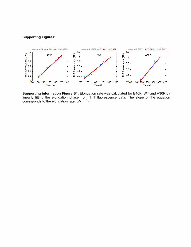
Thioflavin T based assays helped to perceive the α-synuclein aggregation as a nucleation dependent event and that of the two oppositely behaving familial mutants, which have different rates of nucleation that determine their aggregation propensities. The ThT profile was further analyzed to quantify any divergence from the wild type kinetics. Indeed the variants manifest in differential elongation rates of 0.022±0.0004, 0.0118±0.0009 and 0.0049±0.0027 µM-1h-1 for E46K, WT and A30P, respectively (Figure S1 and Table S1).

The change incurred onto the protein backbone owing to the point mutations, lead to a change in the immediate chemical environment of the residues. This change in its immediate environment dictates the backbone orientation of the resultant mutants that show alterations in the resulting secondary structures as was studied qualitatively using CD spectroscopy.18 CD serves to be an excellent method of determining the secondary structure of proteins in solution. However, since the gross structure remains to be unfolded in the early LMW samples, CD spectroscopy does not reveal any secondary conformation corresponding to the primary structure of the three variants. Nevertheless, the change in backbone orientation in the nucleating intermediates of the point mutant forms leads to a change in the alignment of the amide backbone of the resultant chromophores.19 This enables their optical transitions resulting in different characteristic spectra with divergent duration of the helical intermediate formation. In E46K, helix-rich state appeared early but for shorter duration (~20±10 h) whereas in slow aggregating A30P mutant, helix appearance was delayed but it stayed for longer time (Figure S2A) (Table S1). These results are in accordance with the previously published results.20 Furthermore; CD intensity at 218 nm wavelengths versus time was used to trace the kinetics of the intermediate and fibril formation. Intensity at 218 nm increased with increased in incubation time for all the three proteins with β-sheet conversion rate fastest for E46K> WT>A30P (Figure S2B), consistent with the ThT data. The time-dependent structural transitions from random coil to

 

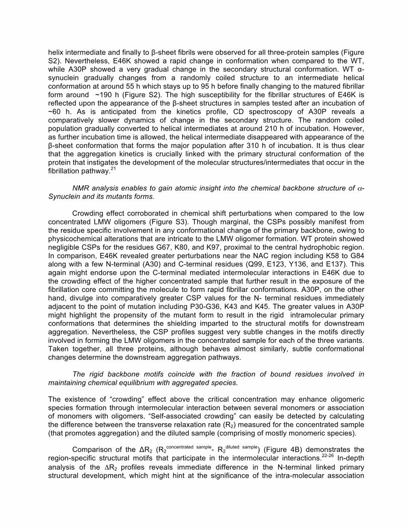
helix intermediate and finally to β-sheet fibrils were observed for all three-protein samples (Figure S2). Nevertheless, E46K showed a rapid change in conformation when compared to the WT, while A30P showed a very gradual change in the secondary structural conformation. WT α-synuclein gradually changes from a randomly coiled structure to an intermediate helical conformation at around 55 h which stays up to 95 h before finally changing to the matured fibrillar form around ~190 h (Figure S2). The high susceptibility for the fibrillar structures of E46K is reflected upon the appearance of the β-sheet structures in samples tested after an incubation of ~60 h. As is anticipated from the kinetics profile, CD spectroscopy of A30P reveals a comparatively slower dynamics of change in the secondary structure. The random coiled population gradually converted to helical intermediates at around 210 h of incubation. However, as further incubation time is allowed, the helical intermediate disappeared with appearance of the β-sheet conformation that forms the major population after 310 h of incubation. It is thus clear that the aggregation kinetics is crucially linked with the primary structural conformation of the protein that instigates the development of the molecular structures/intermediates that occur in the fibrillation pathway.21

NMR analysis enables to gain atomic insight into the chemical backbone structure of α-Synuclein and its mutants forms.

Crowding effect corroborated in chemical shift perturbations when compared to the low concentrated LMW oligomers (Figure S3). Though marginal, the CSPs possibly manifest from the residue specific involvement in any conformational change of the primary backbone, owing to physicochemical alterations that are intricate to the LMW oligomer formation. WT protein showed negligible CSPs for the residues G67, K80, and K97, proximal to the central hydrophobic region. In comparison, E46K revealed greater perturbations near the NAC region including K58 to G84 along with a few N-terminal (A30) and C-terminal residues (Q99, E123, Y136, and E137). This again might endorse upon the C-terminal mediated intermolecular interactions in E46K due to the crowding effect of the higher concentrated sample that further result in the exposure of the fibrillation core committing the molecule to form rapid fibrillar conformations. A30P, on the other hand, divulge into comparatively greater CSP values for the N- terminal residues immediately adjacent to the point of mutation including P30-G36, K43 and K45. The greater values in A30P might highlight the propensity of the mutant form to result in the rigid intramolecular primary conformations that determines the shielding imparted to the structural motifs for downstream aggregation. Nevertheless, the CSP profiles suggest very subtle changes in the motifs directly involved in forming the LMW oligomers in the concentrated sample for each of the three variants. Taken together, all three proteins, although behaves almost similarly, subtle conformational changes determine the downstream aggregation pathways.

The rigid backbone motifs coincide with the fraction of bound residues involved in maintaining chemical equilibrium with aggregated species.

The existence of “crowding” effect above the critical concentration may enhance oligomeric species formation through intermolecular interaction between several monomers or association of monomers with oligomers. “Self-associated crowding” can easily be detected by calculating the difference between the transverse relaxation rate (R2) measured for the concentrated sample (that promotes aggregation) and the diluted sample (comprising of mostly monomeric species).

Comparison of the ΔR2 (R2concentrated sample- R2

diluted sample) (Figure 4B) demonstrates the region-specific structural motifs that participate in the intermolecular interactions.22-26 In-depth analysis of the ΔR2

profiles reveals immediate difference in the N-terminal linked primary structural development, which might hint at the significance of the intra-molecular association

 

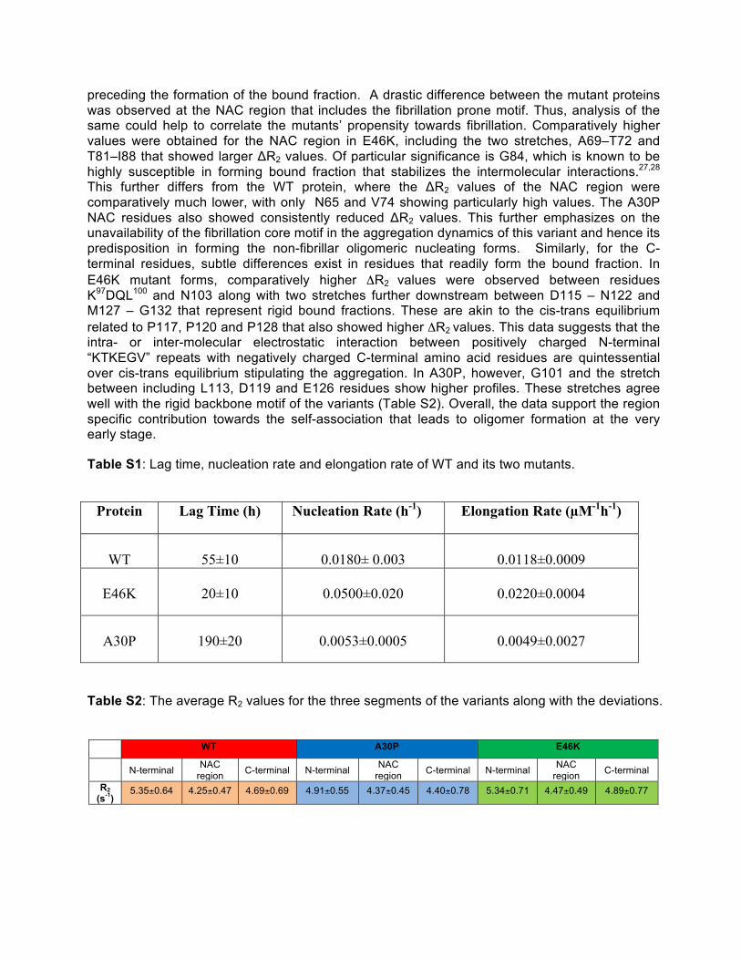
preceding the formation of the bound fraction. A drastic difference between the mutant proteins was observed at the NAC region that includes the fibrillation prone motif. Thus, analysis of the same could help to correlate the mutants’ propensity towards fibrillation. Comparatively higher values were obtained for the NAC region in E46K, including the two stretches, A69–T72 and T81–I88 that showed larger ΔR2 values. Of particular significance is G84, which is known to be highly susceptible in forming bound fraction that stabilizes the intermolecular interactions.27,28 This further differs from the WT protein, where the ΔR2 values of the NAC region were comparatively much lower, with only N65 and V74 showing particularly high values. The A30P NAC residues also showed consistently reduced ΔR2 values. This further emphasizes on the unavailability of the fibrillation core motif in the aggregation dynamics of this variant and hence its predisposition in forming the non-fibrillar oligomeric nucleating forms. Similarly, for the C-terminal residues, subtle differences exist in residues that readily form the bound fraction. In E46K mutant forms, comparatively higher ΔR2

values were observed between residues K97DQL100 and N103 along with two stretches further downstream between D115 – N122 and M127 – G132 that represent rigid bound fractions. These are akin to the cis-trans equilibrium related to P117, P120 and P128 that also showed higher ΔR2 values. This data suggests that the intra- or inter-molecular electrostatic interaction between positively charged N-terminal “KTKEGV” repeats with negatively charged C-terminal amino acid residues are quintessential over cis-trans equilibrium stipulating the aggregation. In A30P, however, G101 and the stretch between including L113, D119 and E126 residues show higher profiles. These stretches agree well with the rigid backbone motif of the variants (Table S2). Overall, the data support the region specific contribution towards the self-association that leads to oligomer formation at the very early stage.

Table S1: Lag time, nucleation rate and elongation rate of WT and its two mutants.

Protein Lag Time (h) Nucleation Rate (h-1) Elongation Rate (µM-1h-1)

WT

55±10

0.0180± 0.003

0.0118±0.0009

E46K

20±10

0.0500±0.020

0.0220±0.0004

A30P

190±20

0.0053±0.0005

0.0049±0.0027

Table S2: The average R2 values for the three segments of the variants along with the deviations.

WT A30P E46K

N-terminal NAC region C-terminal N-terminal NAC

region C-terminal N-terminal NAC region C-terminal

R2 (s-1)

5.35±0.64 4.25±0.47 4.69±0.69 4.91±0.55 4.37±0.45 4.40±0.78 5.34±0.71 4.47±0.49 4.89±0.77

 

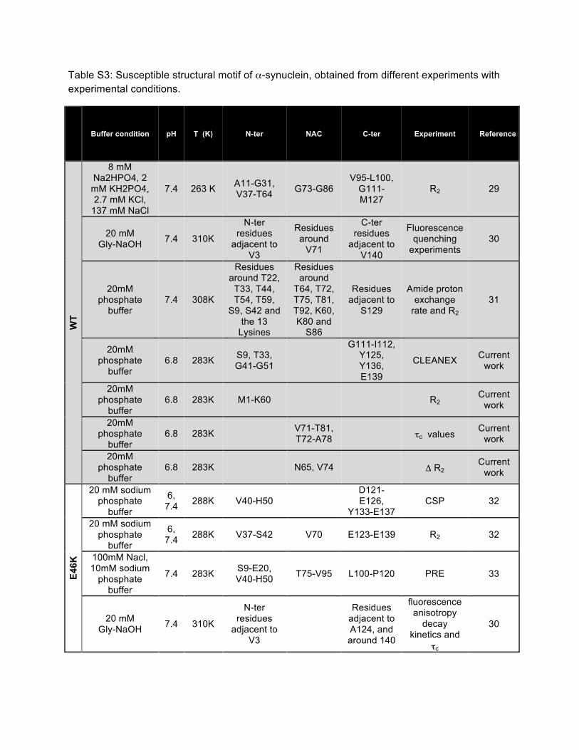
Table S3: Susceptible structural motif of α-synuclein, obtained from different experiments with experimental conditions.

Buffer condition pH T (K) N-ter NAC C-ter Experiment Reference

WT

8 mM Na2HPO4, 2 mM KH2PO4, 2.7 mM KCl,

137 mM NaCl

7.4 263 K A11-G31, V37-T64 G73-G86

V95-L100, G111-M127

R2 29

20 mM Gly-NaOH 7.4 310K

N-ter residues

adjacent to V3

Residues around

V71

C-ter residues

adjacent to V140

Fluorescence quenching

experiments 30

20mM phosphate

buffer 7.4 308K

Residues around T22,

T33, T44, T54, T59,

S9, S42 and the 13

Lysines

Residues around

T64, T72, T75, T81, T92, K60, K80 and

S86

Residues adjacent to

S129

Amide proton exchange

rate and R2 31

20mM phosphate

buffer 6.8 283K S9, T33,

G41-G51

G111-I112, Y125, Y136, E139

CLEANEX Current work

20mM phosphate

buffer 6.8 283K M1-K60 R2

Current work

20mM phosphate

buffer 6.8 283K

V71-T81, T72-A78 τc values Current

work

20mM phosphate

buffer 6.8 283K N65, V74 Δ R2

Current work

E46K

20 mM sodium phosphate

buffer

6, 7.4 288K V40-H50

D121-E126,

Y133-E137 CSP 32

20 mM sodium phosphate

buffer

6, 7.4 288K V37-S42 V70 E123-E139 R2 32

100mM Nacl, 10mM sodium

phosphate buffer

7.4 283K S9-E20, V40-H50 T75-V95 L100-P120 PRE 33

20 mM Gly-NaOH 7.4 310K

N-ter residues

adjacent to V3

Residues adjacent to A124, and around 140

fluorescence anisotropy

decay kinetics and

τc

30

 

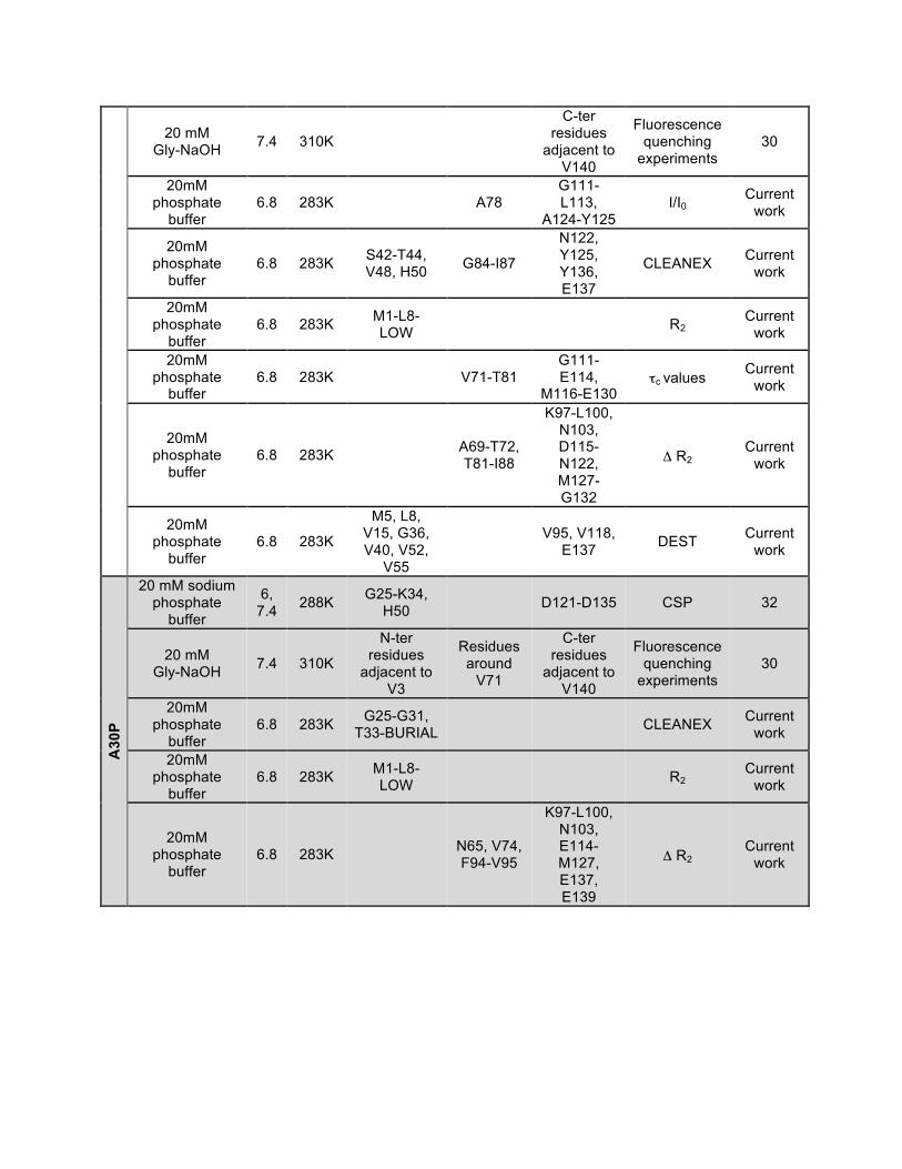
20 mM Gly-NaOH 7.4 310K

C-ter residues

adjacent to V140

Fluorescence quenching

experiments 30

20mM phosphate

buffer 6.8 283K A78

G111-L113,

A124-Y125 I/I0

Current work

20mM phosphate

buffer 6.8 283K S42-T44,

V48, H50 G84-I87

N122, Y125, Y136, E137

CLEANEX Current work

20mM phosphate

buffer 6.8 283K M1-L8-

LOW R2 Current

work

20mM phosphate

buffer 6.8 283K V71-T81

G111-E114,

M116-E130 τc values Current

work

20mM phosphate

buffer 6.8 283K

A69-T72, T81-I88

K97-L100, N103, D115-N122, M127-G132

Δ R2 Current

work

20mM phosphate

buffer 6.8 283K

M5, L8, V15, G36, V40, V52,

V55

V95, V118, E137 DEST Current

work

A30

P

20 mM sodium phosphate

buffer

6, 7.4 288K G25-K34,

H50 D121-D135 CSP 32

20 mM Gly-NaOH 7.4 310K

N-ter residues

adjacent to V3

Residues around

V71

C-ter residues

adjacent to V140

Fluorescence quenching

experiments 30

20mM phosphate

buffer 6.8 283K G25-G31,

T33-BURIAL CLEANEX Current work

20mM phosphate

buffer 6.8 283K M1-L8-

LOW R2 Current

work

20mM phosphate

buffer 6.8 283K

N65, V74, F94-V95

K97-L100, N103, E114-M127, E137, E139

Δ R2 Current

work

 

 

Supporting Figures:

Supporting information Figure S1. Elongation rate was calculated for E46K, WT and A30P by linearly fitting the elongation phase from ThT fluorescence data. The slope of the equation corresponds to the elongation rate (µM-1h-1).

 

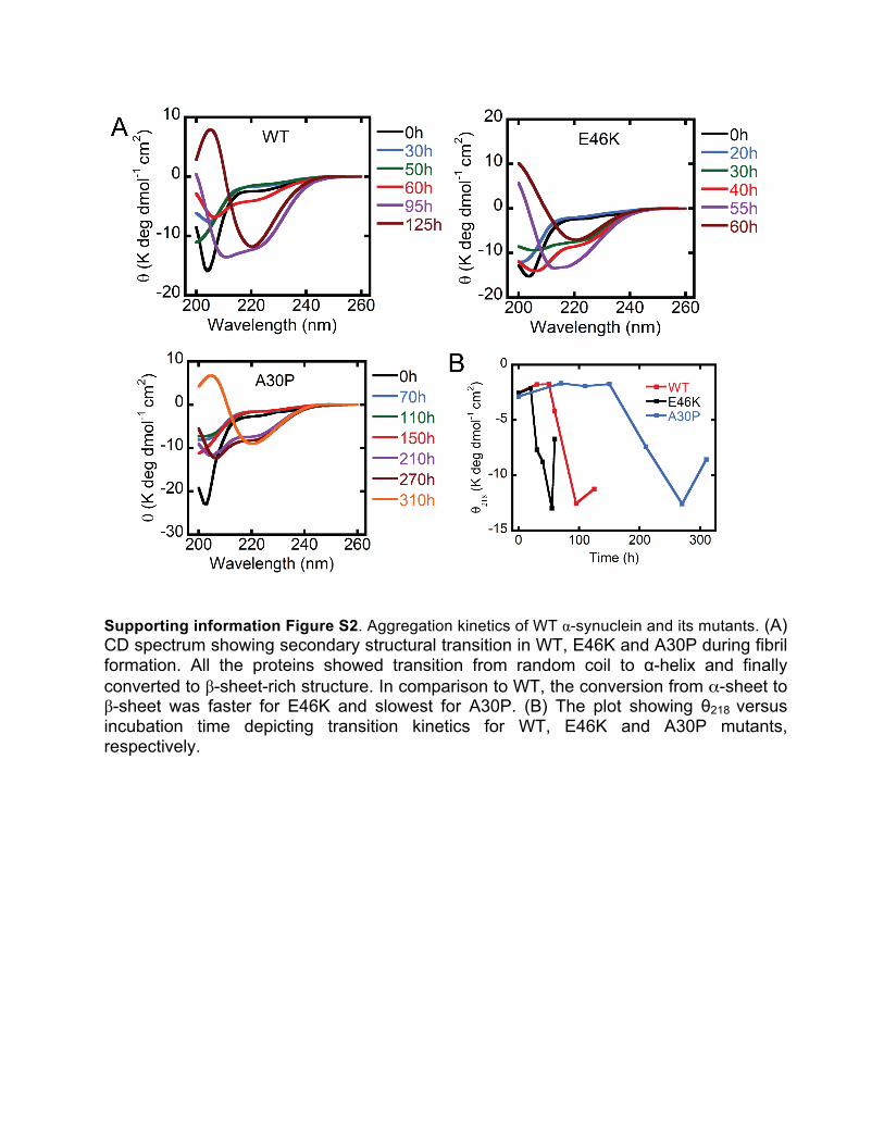
Supporting information Figure S2. Aggregation kinetics of WT α-synuclein and its mutants. (A) CD spectrum showing secondary structural transition in WT, E46K and A30P during fibril formation. All the proteins showed transition from random coil to α-helix and finally converted to β-sheet-rich structure. In comparison to WT, the conversion from α-sheet to β-sheet was faster for E46K and slowest for A30P. (B) The plot showing θ218 versus incubation time depicting transition kinetics for WT, E46K and A30P mutants, respectively.

 

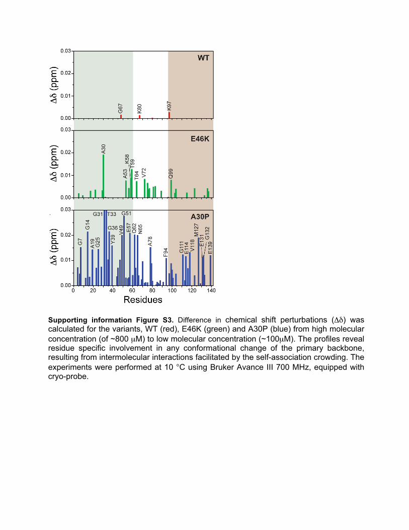
Supporting information Figure S3. Difference in chemical shift perturbations (Δδ) was calculated for the variants, WT (red), E46K (green) and A30P (blue) from high molecular concentration (of ~800 µM) to low molecular concentration (~100µM). The profiles reveal  residue specific involvement in any conformational change of the primary backbone, resulting from intermolecular interactions facilitated by the self-association crowding. The experiments were performed at 10 °C using Bruker Avance III 700 MHz, equipped with cryo-probe.

 

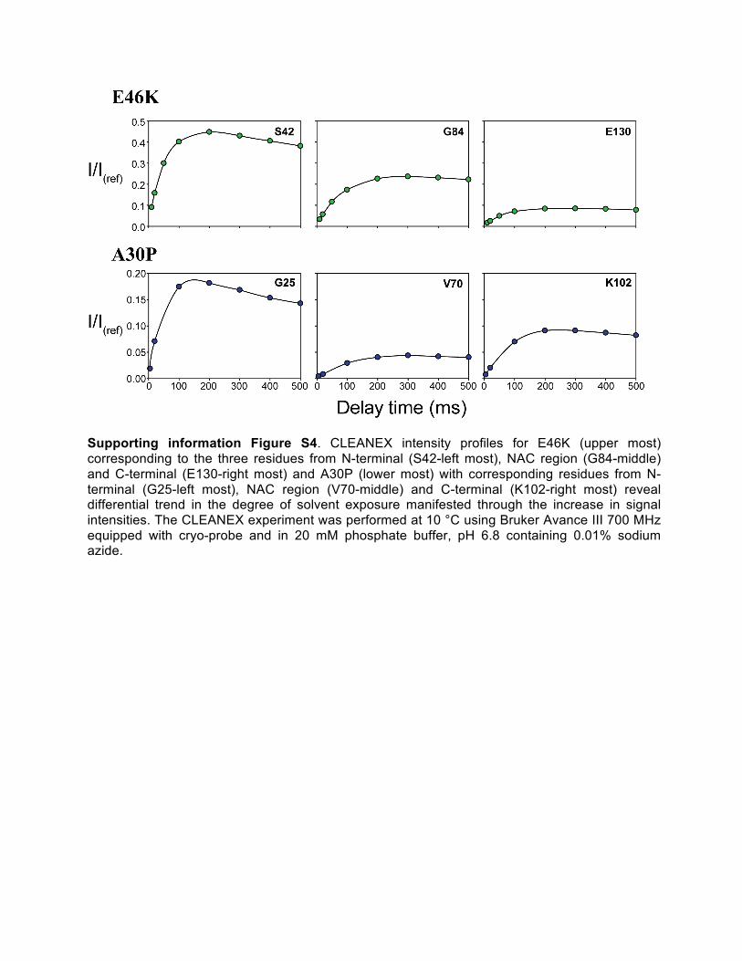
Supporting information Figure S4. CLEANEX intensity profiles for E46K (upper most) corresponding to the three residues from N-terminal (S42-left most), NAC region (G84-middle) and C-terminal (E130-right most) and A30P (lower most) with corresponding residues from N-terminal (G25-left most), NAC region (V70-middle) and C-terminal (K102-right most) reveal differential trend in the degree of solvent exposure manifested through the increase in signal intensities. The CLEANEX experiment was performed at 10 °C using Bruker Avance III 700 MHz equipped with cryo-probe and in 20 mM phosphate buffer, pH 6.8 containing 0.01% sodium azide.

 

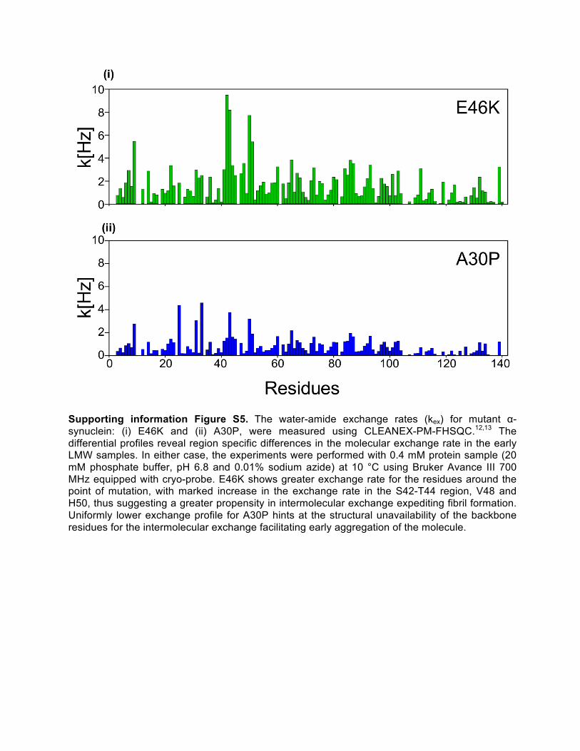
Supporting information Figure S5.   The water-amide exchange rates (kex) for mutant α-synuclein: (i) E46K and (ii) A30P, were measured using CLEANEX-PM-FHSQC.12,13 The differential profiles reveal region specific differences in the molecular exchange rate in the early LMW samples. In either case, the experiments were performed with 0.4 mM protein sample (20 mM phosphate buffer, pH 6.8 and 0.01% sodium azide) at 10 °C using Bruker Avance III 700 MHz equipped with cryo-probe. E46K shows greater exchange rate for the residues around the point of mutation, with marked increase in the exchange rate in the S42-T44 region, V48 and H50, thus suggesting a greater propensity in intermolecular exchange expediting fibril formation. Uniformly lower exchange profile for A30P hints at the structural unavailability of the backbone residues for the intermolecular exchange facilitating early aggregation of the molecule.

 

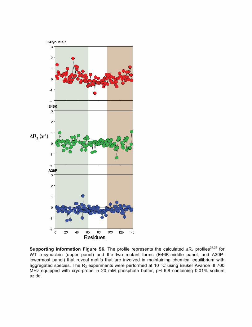
Supporting information Figure S6. The profile represents the calculated ΔR2 profiles24,26 for WT α-synuclein (upper panel) and the two mutant forms (E46K-middle panel, and A30P- lowermost panel) that reveal motifs that are involved in maintaining chemical equilibrium with aggregated species. The R2 experiments were performed at 10 °C using Bruker Avance III 700 MHz equipped with cryo-probe in 20 mM phosphate buffer, pH 6.8 containing 0.01% sodium azide.

 

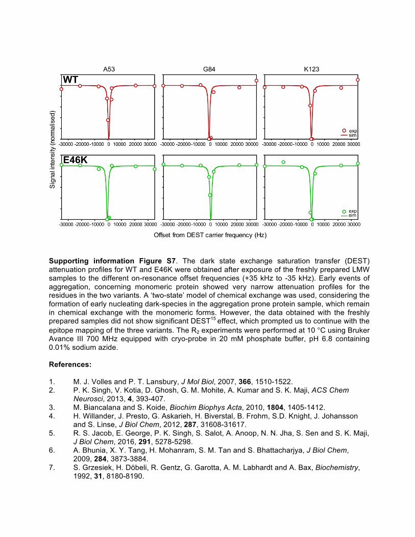
Supporting information Figure S7. The dark state exchange saturation transfer (DEST) attenuation profiles for WT and E46K were obtained after exposure of the freshly prepared LMW samples to the different on-resonance offset frequencies (+35 kHz to -35 kHz). Early events of aggregation, concerning monomeric protein showed very narrow attenuation profiles for the residues in the two variants. A ‘two-state’ model of chemical exchange was used, considering the formation of early nucleating dark-species in the aggregation prone protein sample, which remain in chemical exchange with the monomeric forms. However, the data obtained with the freshly prepared samples did not show significant DEST15 effect, which prompted us to continue with the epitope mapping of the three variants. The R2 experiments were performed at 10 °C using Bruker Avance III 700 MHz equipped with cryo-probe in 20 mM phosphate buffer, pH 6.8 containing 0.01% sodium azide. References: 1. M. J. Volles and P. T. Lansbury, J Mol Biol, 2007, 366, 1510-1522. 2. P. K. Singh, V. Kotia, D. Ghosh, G. M. Mohite, A. Kumar and S. K. Maji, ACS Chem

Neurosci, 2013, 4, 393-407. 3. M. Biancalana and S. Koide, Biochim Biophys Acta, 2010, 1804, 1405-1412. 4. H. Willander, J. Presto, G. Askarieh, H. Biverstal, B. Frohm, S.D. Knight, J. Johansson

and S. Linse, J Biol Chem, 2012, 287, 31608-31617. 5. R. S. Jacob, E. George, P. K. Singh, S. Salot, A. Anoop, N. N. Jha, S. Sen and S. K. Maji,

J Biol Chem, 2016, 291, 5278-5298. 6. A. Bhunia, X. Y. Tang, H. Mohanram, S. M. Tan and S. Bhattacharjya, J Biol Chem,

2009, 284, 3873-3884. 7. S. Grzesiek, H. Döbeli, R. Gentz, G. Garotta, A. M. Labhardt and A. Bax, Biochemistry,

1992, 31, 8180-8190.

 

8. J. R. Brender, J. Krishnamoorthy, M. F. Sciacca, S. Vivekanandan, L. D'Urso, J. Chen, C. La Rosa and A. Ramamoorthy, J Phys Chem B, 2015, 119, 2886-2896.

9. N. A. Farrow, R. Muhandiram, A. U. Singer, S. M. Pascal, C. M. Kay, G. Gish, S. E. Shoelson, T. Pawson, J. D. Forman-Kay and L. E. Kay, Biochemistry, 1994, 33, 5984-6003.

10. S. Gupta and S. Bhattacharjya, Proteins, 2014, 82, 2957-2969. 11. M. R. Gryk, R. Abseher, B. Simon, M. Nilges and H. Oschkinat, J Mol Biol, 1998, 280,

879-896. 12. A. Bhunia, P. N. Domadia, H. Mohanram and S. Bhattacharjya, Proteins, 2009, 74, 328-

343. 13. T. L. Hwang, P. C. van Zijl and S. Mori, J Biomol NMR, 1998, 11, 221-226. 14. N. Rezaei-Ghaleh, E. Andreetto, L. M. Yan, A. Kapurniotu and M. Zweckstetter, PLoS

One, 2011, 6, e20289. 15. N. L. Fawzi, J. Ying, D. A. Torchia and G. M. Clore, Nat Protoc, 2012, 7, 1523-1533. 16. N. L. Fawzi, J. Ying, R. Ghirlando, D. A. Torchia and G. M. Clore, Nature, 2011, 480, 268-

272. 17. N. L. Fawzi, D. S. Libich, J. Ying, V. Tugarinov and G. M. Clore, Angew Chem Int Ed

Engl, 2014, 53, 10345-10349. 18. N. J. Greenfield, Nat Protoc, 2006, 1, 2876-2890. 19. O. V. Stepanenko, I. M. Kuznetsova, V. V. Verkhusha and K. K. Turoverov, Int Rev Cell

Mol Biol, 2013, 302, 221-278. 20 D. Ghosh, P. K. Singh, S. Sahay, N. N. Jha, R. S. Jacob, S. Sen, A. Kumar, R. Riek and

S. K. Maji, Sci Rep, 2015, 5, 9228. 21. K. A. Conway, S. J. Lee, J. C. Rochet, T. T. Ding, R. E. Williamson and P. T. Lansbury,

Proc Natl Acad Sci U S A, 2000, 97, 571-576. 22. Y. Song, A. K. Kenworthy and C. R. Sanders, Protein Sci, 2014, 23, 1-22. 23. C. R. Bodner, A. S. Maltsev, C. M. Dobson and A. Bax, Biochemistry, 2010, 49, 862-871. 24. N. L. Fawzi, J. Ying, D. A. Torchia and G. M. Clore, J Am Chem Soc, 2010, 132, 9948-

9951. 25. B. VanSchouwen, R. Selvaratnam, R. Giri, R. Lorenz, F. W. Herberg, C. Kim and G.

Melacini, J Biol Chem, 2015, 290, 28631-28641. 26. A. Ceccon, V. Tugarinov, A. J. Boughton, D. Fushman and G. M. Clore, J Phys Chem

Lett, 2017, 8, 2535-2540. 27. R. Harada, N. Kobayashi, J. Kim, C. Nakamura, S. W. Han, K. Ikebukuro and K. Sode,

Biochim Biophys Acta, 2009, 1792, 998-1003. 28. O. Wise-Scira, A. Dunn, A. K. Aloglu, I. T. Sakallioglu and O. Coskuner, ACS Chem

Neurosci, 2013, 4, 498-508. 29. K. P. Wu, S. Kim, D. A. Fela and J. Baum, J Mol Biol, 2008, 378, 1104-1115. 30. S. Sahay, D. Ghosh, S. Dwivedi, A. Anoop, G. M. Mohite, M. Kombrabail, G.

Krishnamoorthy and S. K. Maji, J Biol Chem, 2015, 290, 7804-7822. 31. R. L. Croke, C. O. Sallum, E. Watson, E. D. Watt and A. T. Alexandrescu, Protein Sci,

2008, 17, 1434-1445. 32. P. Ranjan and A. Kumar, ACS Chem Neurosci, 2017. 33. C. C. Rospigliosi, S. McClendon, A. W. Schmid, T. F. Ramlall, P. Barré, H. A. Lashuel

and D. Eliezer, J Mol Biol, 2009, 388, 1022-1032.