arX

iv:0

808.

0746

v1 [

hep-

th]

5 A

ug 2

008

1

Progress of Theoretical Physics, Vol. 111, No. 4, April 2004

String Gas Cosmology

LATEX2ε Version

Robert H. Brandenberger∗)

Physics Department, McGill University, Montreal, QC, H3T 2A8, Canada

(Received August 4, 2008)

String gas cosmology is a string theory-based approach to early universe cosmology whichis based on making use of robust features of string theory such as the existence of new statesand new symmetries. A first goal of string gas cosmology is to understand how string theorycan effect the earliest moments of cosmology before the effective field theory approach whichunderlies standard and inflationary cosmology becomes valid. String gas cosmology mayalso provide an alternative to the current standard paradigm of cosmology, the inflationaryuniverse scenario. Here, the current status of string gas cosmology is reviewed.

§1. Introduction

1.1. The Current Paradigm of Early Universe Cosmology

According to the inflationary universe scenario1) (see also2)–4)), there was a phaseof accelerated expansion of space lasting at least 50 Hubble expansion times duringthe very early universe. This accelerated expansion of space can explain the overallhomogeneity of the universe, it can explain its large size and entropy, and it leads toa decrease in the curvature of space. Most importantly, however, it includes a causalmechanism for generating the small amplitude fluctuations which can be mapped outtoday via the induced temperature fluctuations of the cosmic microwave background(CMB) and which develop into the observed large-scale structure of the universe5)

(see also2), 6)–8)). The accelerated expansion of space stretches fixed co-moving scalesbeyond the Hubble radius. Thus, it is possible to have a causal mechanism whichgenerates the fluctuations on microscopic sub-Hubble scales. The wavelengths ofthese inhomogeneities are subsequently inflated to cosmological scales which aresuper-Hubble until the late universe. The generation mechanism is based on theassumption that the fluctuations start out on microscopic scales at the beginningof the period of inflation in a quantum vacuum state. If the expansion of space isalmost exponential, an almost scale-invariant spectrum of cosmological perturbationsresults, and the squeezing which the fluctuations undergo while they evolve on scaleslarger than the Hubble radius predicts a characteristic oscillatory pattern in theangular power spectrum of the CMB anisotropies,9) a pattern which has now beenconfirmed with great accuracy10), 11) (see e.g12) for a comprehensive review of thetheory of cosmological fluctuations, and13) for an introductory overview).

To establish our notation, we write the metric of a homogeneous, isotropic and

∗) E-mail: rhb@hep.physics.mcgill.ca

typeset using PTPTEX.cls 〈Ver.0.9〉

2 R. Brandenberger

spatially flat four-dimensional universe in the form

ds2 = dt2 − a(t)2dx2 , (1.1)

where t is physical time, x denote the three co-moving spatial coordinates (pointsat rest in an expanding space have constant co-moving coordinates), and the scalefactor a(t) is proportional to the size of space. The expansion rate H(t) of theuniverse is given by

H(t) =a

a, (1.2)

where the overdot represents the derivative with respect to time.

t

xt R

t 0

t i

t f (k)

t i (k)

k

H −1

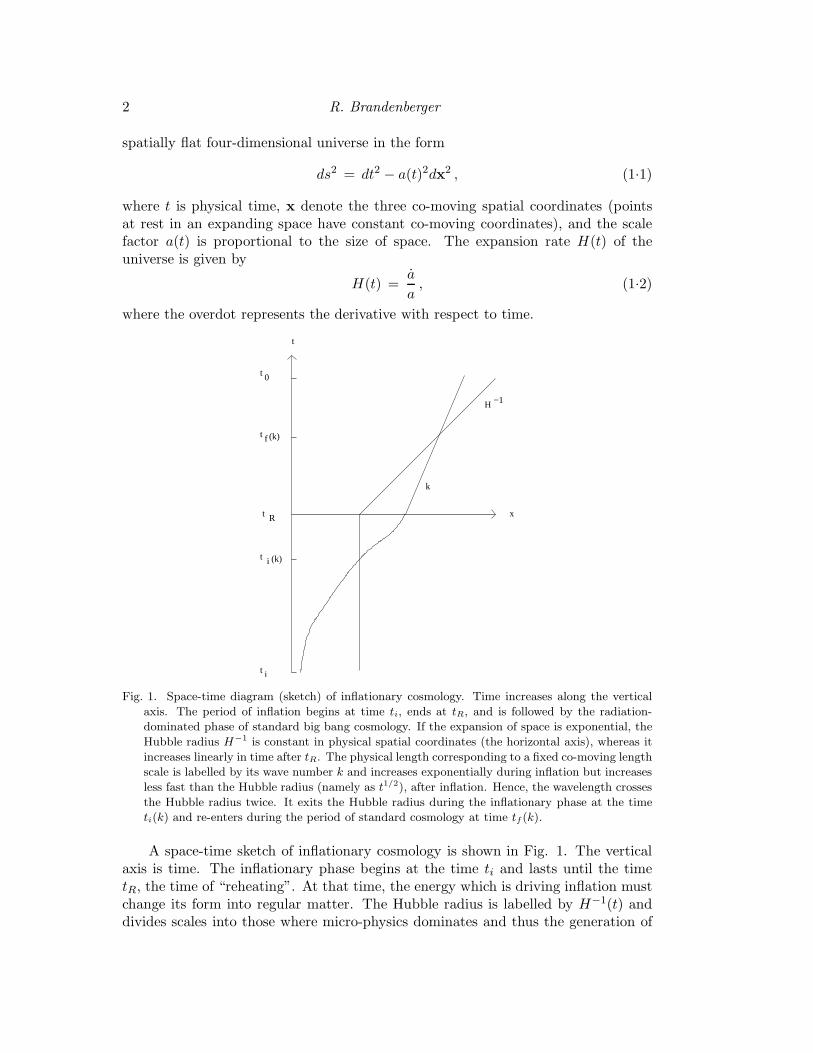
Fig. 1. Space-time diagram (sketch) of inflationary cosmology. Time increases along the vertical

axis. The period of inflation begins at time ti, ends at tR, and is followed by the radiation-

dominated phase of standard big bang cosmology. If the expansion of space is exponential, the

Hubble radius H−1 is constant in physical spatial coordinates (the horizontal axis), whereas it

increases linearly in time after tR. The physical length corresponding to a fixed co-moving length

scale is labelled by its wave number k and increases exponentially during inflation but increases

less fast than the Hubble radius (namely as t1/2), after inflation. Hence, the wavelength crosses

the Hubble radius twice. It exits the Hubble radius during the inflationary phase at the time

ti(k) and re-enters during the period of standard cosmology at time tf (k).

A space-time sketch of inflationary cosmology is shown in Fig. 1. The verticalaxis is time. The inflationary phase begins at the time ti and lasts until the timetR, the time of “reheating”. At that time, the energy which is driving inflation mustchange its form into regular matter. The Hubble radius is labelled by H−1(t) anddivides scales into those where micro-physics dominates and thus the generation of

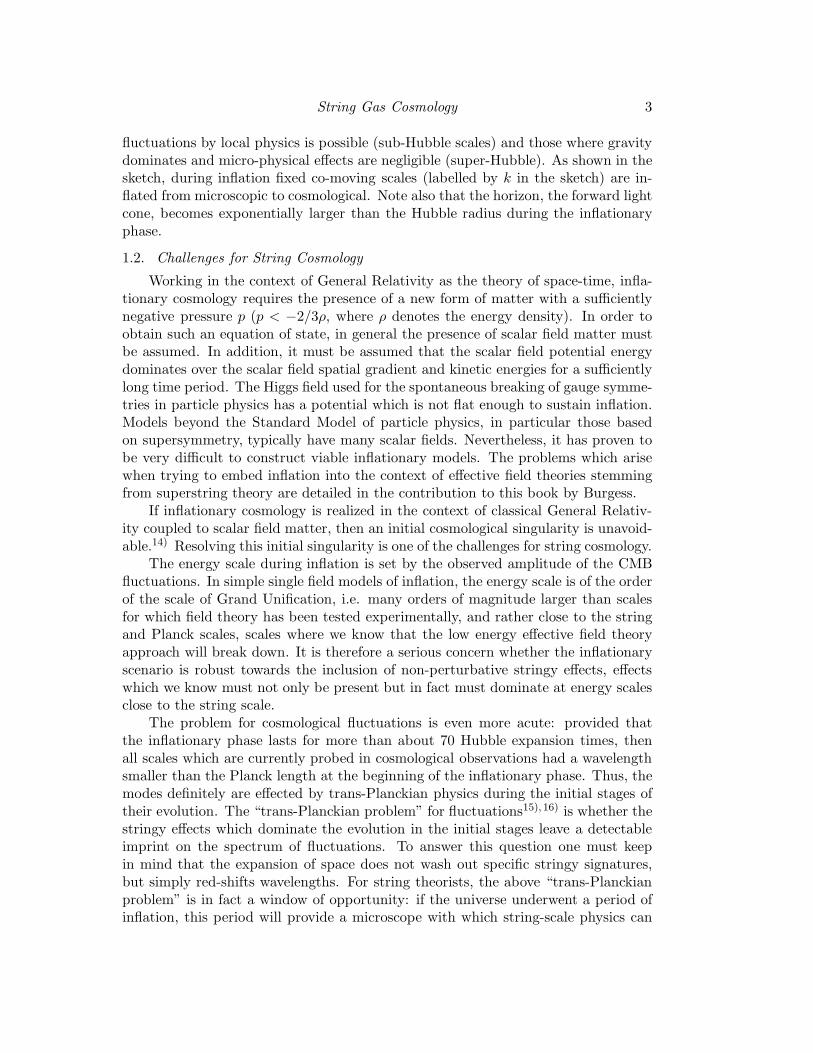
String Gas Cosmology 3

fluctuations by local physics is possible (sub-Hubble scales) and those where gravitydominates and micro-physical effects are negligible (super-Hubble). As shown in thesketch, during inflation fixed co-moving scales (labelled by k in the sketch) are in-flated from microscopic to cosmological. Note also that the horizon, the forward lightcone, becomes exponentially larger than the Hubble radius during the inflationaryphase.

1.2. Challenges for String Cosmology

Working in the context of General Relativity as the theory of space-time, infla-tionary cosmology requires the presence of a new form of matter with a sufficientlynegative pressure p (p < −2/3ρ, where ρ denotes the energy density). In order toobtain such an equation of state, in general the presence of scalar field matter mustbe assumed. In addition, it must be assumed that the scalar field potential energydominates over the scalar field spatial gradient and kinetic energies for a sufficientlylong time period. The Higgs field used for the spontaneous breaking of gauge symme-tries in particle physics has a potential which is not flat enough to sustain inflation.Models beyond the Standard Model of particle physics, in particular those basedon supersymmetry, typically have many scalar fields. Nevertheless, it has proven tobe very difficult to construct viable inflationary models. The problems which arisewhen trying to embed inflation into the context of effective field theories stemmingfrom superstring theory are detailed in the contribution to this book by Burgess.

If inflationary cosmology is realized in the context of classical General Relativ-ity coupled to scalar field matter, then an initial cosmological singularity is unavoid-able.14) Resolving this initial singularity is one of the challenges for string cosmology.

The energy scale during inflation is set by the observed amplitude of the CMBfluctuations. In simple single field models of inflation, the energy scale is of the orderof the scale of Grand Unification, i.e. many orders of magnitude larger than scalesfor which field theory has been tested experimentally, and rather close to the stringand Planck scales, scales where we know that the low energy effective field theoryapproach will break down. It is therefore a serious concern whether the inflationaryscenario is robust towards the inclusion of non-perturbative stringy effects, effectswhich we know must not only be present but in fact must dominate at energy scalesclose to the string scale.

The problem for cosmological fluctuations is even more acute: provided thatthe inflationary phase lasts for more than about 70 Hubble expansion times, thenall scales which are currently probed in cosmological observations had a wavelengthsmaller than the Planck length at the beginning of the inflationary phase. Thus, themodes definitely are effected by trans-Planckian physics during the initial stages oftheir evolution. The “trans-Planckian problem” for fluctuations15), 16) is whether thestringy effects which dominate the evolution in the initial stages leave a detectableimprint on the spectrum of fluctuations. To answer this question one must keepin mind that the expansion of space does not wash out specific stringy signatures,but simply red-shifts wavelengths. For string theorists, the above “trans-Planckianproblem” is in fact a window of opportunity: if the universe underwent a period ofinflation, this period will provide a microscope with which string-scale physics can

4 R. Brandenberger

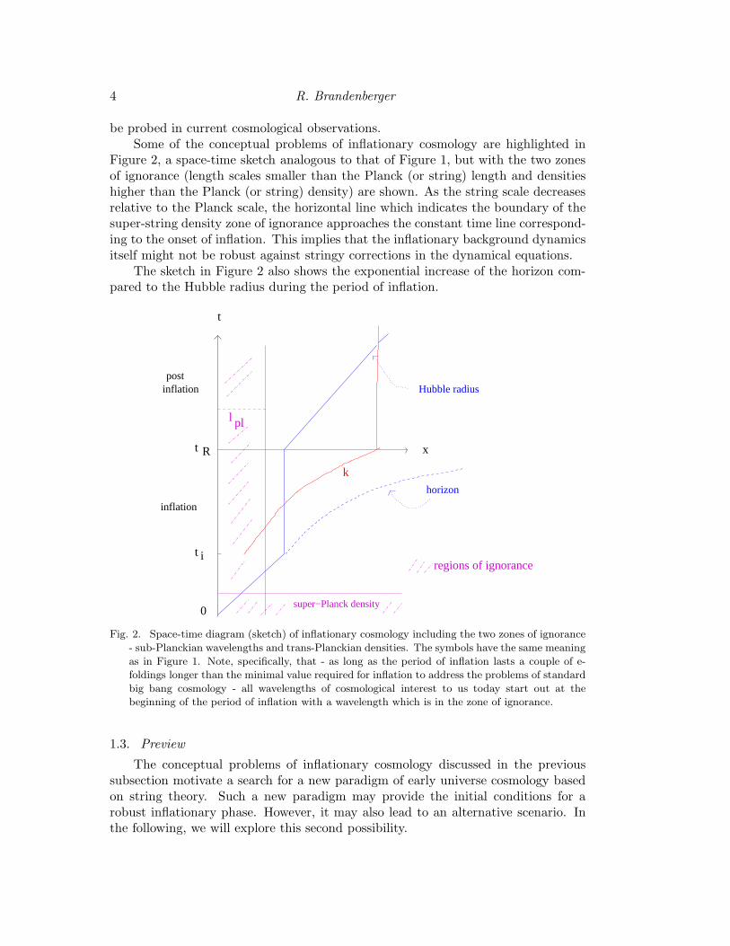
be probed in current cosmological observations.Some of the conceptual problems of inflationary cosmology are highlighted in

Figure 2, a space-time sketch analogous to that of Figure 1, but with the two zonesof ignorance (length scales smaller than the Planck (or string) length and densitieshigher than the Planck (or string) density) are shown. As the string scale decreasesrelative to the Planck scale, the horizontal line which indicates the boundary of thesuper-string density zone of ignorance approaches the constant time line correspond-ing to the onset of inflation. This implies that the inflationary background dynamicsitself might not be robust against stringy corrections in the dynamical equations.

The sketch in Figure 2 also shows the exponential increase of the horizon com-pared to the Hubble radius during the period of inflation.

t

x

t i

t R

inflation

postinflation

horizon

Hubble radius

k

0

l pl

super−Planck density

regions of ignorance

Fig. 2. Space-time diagram (sketch) of inflationary cosmology including the two zones of ignorance

- sub-Planckian wavelengths and trans-Planckian densities. The symbols have the same meaning

as in Figure 1. Note, specifically, that - as long as the period of inflation lasts a couple of e-

foldings longer than the minimal value required for inflation to address the problems of standard

big bang cosmology - all wavelengths of cosmological interest to us today start out at the

beginning of the period of inflation with a wavelength which is in the zone of ignorance.

1.3. Preview

The conceptual problems of inflationary cosmology discussed in the previoussubsection motivate a search for a new paradigm of early universe cosmology basedon string theory. Such a new paradigm may provide the initial conditions for arobust inflationary phase. However, it may also lead to an alternative scenario. Inthe following, we will explore this second possibility.

String Gas Cosmology 5

In the best possible world, the initial phase of string cosmology will eliminate thecosmological “Big Bang” singularity, it will provide a unified description of space,time and matter, and it will allow a controlled computation of the induced cosmo-logical perturbations. The development of such a consistent framework of stringcosmology will, however, have to be based on a consistent understanding of non-perturbative string theory. Such an understanding is at the present time not avail-able.

Given the lack of such an understanding, most approaches to string cosmologyare based on treating matter using an effective field theory description motivatedby string theory. However, in such approaches key features of string theory whichare not present in field theory cannot be seen. The approach to string cosmologydiscussed below is, in contrast, based on studying effects of new degrees of freedomand new symmetries which are key ingredients to string theory, which will be presentin any non-perturbative formulation of string theory.

§2. Basics of String Gas Cosmology

2.1. Principles of String Gas Cosmology

In the absence of a non-perturbative formulation of string theory, the approachto string cosmology which we have suggested, string gas cosmology17)–19) (see also,20)

and22), 23) for reviews), is to focus on symmetries and degrees of freedom which arenew to string theory (compared to point particle theories) and which will be partof any non-perturbative string theory, and to use them to develop a new cosmology.The symmetry we make use of is T-duality, and the new degrees of freedom are thestring oscillatory modes and the string winding modes.

String gas cosmology is based on coupling a classical background which includesthe graviton and the dilaton fields to a gas of strings (and possibly other basic degreesof freedom of string theory such as “branes”). All dimensions of space are taken tobe compact, for reasons which will become clear later. For simplicity, we take allspatial directions to be toroidal and denote the radius of the torus by R. Strings havethree types of states: momentum modes which represent the center of mass motionof the string, oscillatory modes which represent the fluctuations of the strings, andwinding modes counting the number of times a string wraps the torus.

Since the number of string oscillatory states increases exponentially with en-ergy, there is a limiting temperature for a gas of strings in thermal equilibrium, theHagedorn temperature24) TH . Thus, if we take a box of strings and adiabaticallydecrease the box size, the temperature will never diverge. This is the first indicationthat string theory has the potential to resolve the cosmological singularity problem(see also25), 26) for discussions on how the temperature singularity can be avoided instring cosmology).

The second key feature of string theory upon which string gas cosmology is basedis T-duality. To introduce this symmetry, let us discuss the radius dependence of theenergy of the basic string states: The energy of an oscillatory mode is independent

6 R. Brandenberger

of R, momentum mode energies are quantized in units of 1/R, i.e.

En = n1

R, (2.1)

and winding mode energies are quantized in units of R, i.e.

Em = mR , (2.2)

where both n and m are integers. Thus, a new symmetry of the spectrum of stringstates emerges: Under the change

R → 1/R (2.3)

in the radius of the torus (in units of the string length ls) the energy spectrum ofstring states is invariant if winding and momentum quantum numbers are inter-changed

(n,m) → (m,n) . (2.4)

The above symmetry is the simplest element of a larger symmetry group, the T-duality symmetry group which in general also mixes fluxes and geometry. The stringvertex operators are consistent with this symmetry, and thus T-duality is a symmetryof perturbative string theory. Postulating that T-duality extends to non-perturbativestring theory leads27) to the need of adding D-branes to the list of fundamentalobjects in string theory. With this addition, T-duality is expected to be a symmetryof non-perturbative string theory. Specifically, T-duality will take a spectrum ofstable Type IIA branes and map it into a corresponding spectrum of stable TypeIIB branes with identical masses.28)

As discussed in,17) the above T-duality symmetry leads to an equivalence be-tween small and large spaces, an equivalence elaborated on further in.29), 30)

2.2. Dynamics of String Gas Cosmology

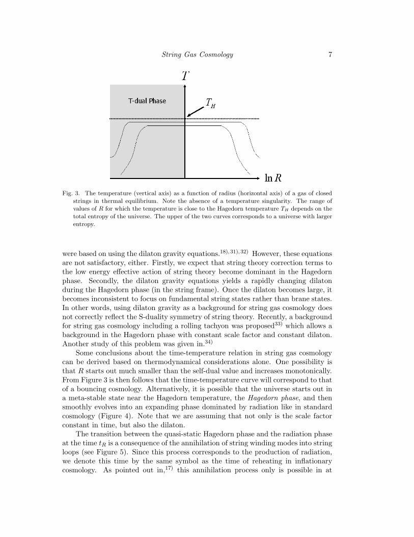
That string gas cosmology will lead to a dynamical evolution of the early uni-verse very different from what is obtained in standard and inflationary cosmologycan already be seen by combining the basic ingredients from string theory discussedin the previous subsection. As the radius of a box of strings decreases from an ini-tially very large value - maintaining thermal equilibrium - , the temperature firstrises as in standard cosmology since the string states which are occupied (the mo-mentum modes) get heavier. However, as the temperature approaches the Hagedorntemperature, the energy begins to flow into the oscillatory modes and the increasein temperature levels off. As the radius R decreases below the string scale, the tem-perature begins to decrease as the energy begins to flow into the winding modeswhose energy decreases as R decreases (see Figure 3). Thus, as argued in,17) thetemperature singularity of early universe cosmology should be resolved in string gascosmology.

The equations that govern that background of string gas cosmology are notknown. The Einstein equations are not the correct equations since they do not obeythe T-duality symmetry of string theory. Many early studies of string gas cosmology

String Gas Cosmology 7

Fig. 3. The temperature (vertical axis) as a function of radius (horizontal axis) of a gas of closed

strings in thermal equilibrium. Note the absence of a temperature singularity. The range of

values of R for which the temperature is close to the Hagedorn temperature TH depends on the

total entropy of the universe. The upper of the two curves corresponds to a universe with larger

entropy.

were based on using the dilaton gravity equations.18), 31), 32) However, these equationsare not satisfactory, either. Firstly, we expect that string theory correction terms tothe low energy effective action of string theory become dominant in the Hagedornphase. Secondly, the dilaton gravity equations yields a rapidly changing dilatonduring the Hagedorn phase (in the string frame). Once the dilaton becomes large, itbecomes inconsistent to focus on fundamental string states rather than brane states.In other words, using dilaton gravity as a background for string gas cosmology doesnot correctly reflect the S-duality symmetry of string theory. Recently, a backgroundfor string gas cosmology including a rolling tachyon was proposed33) which allows abackground in the Hagedorn phase with constant scale factor and constant dilaton.Another study of this problem was given in.34)

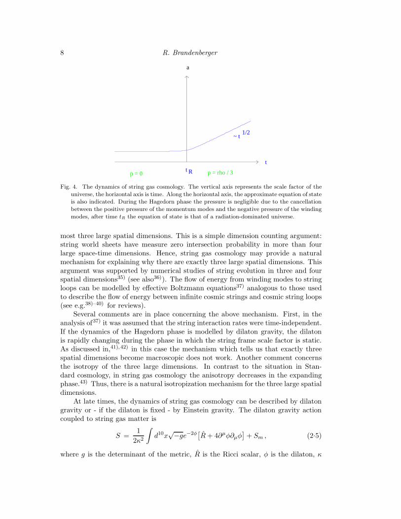
Some conclusions about the time-temperature relation in string gas cosmologycan be derived based on thermodynamical considerations alone. One possibility isthat R starts out much smaller than the self-dual value and increases monotonically.From Figure 3 is then follows that the time-temperature curve will correspond to thatof a bouncing cosmology. Alternatively, it is possible that the universe starts out ina meta-stable state near the Hagedorn temperature, the Hagedorn phase, and thensmoothly evolves into an expanding phase dominated by radiation like in standardcosmology (Figure 4). Note that we are assuming that not only is the scale factorconstant in time, but also the dilaton.

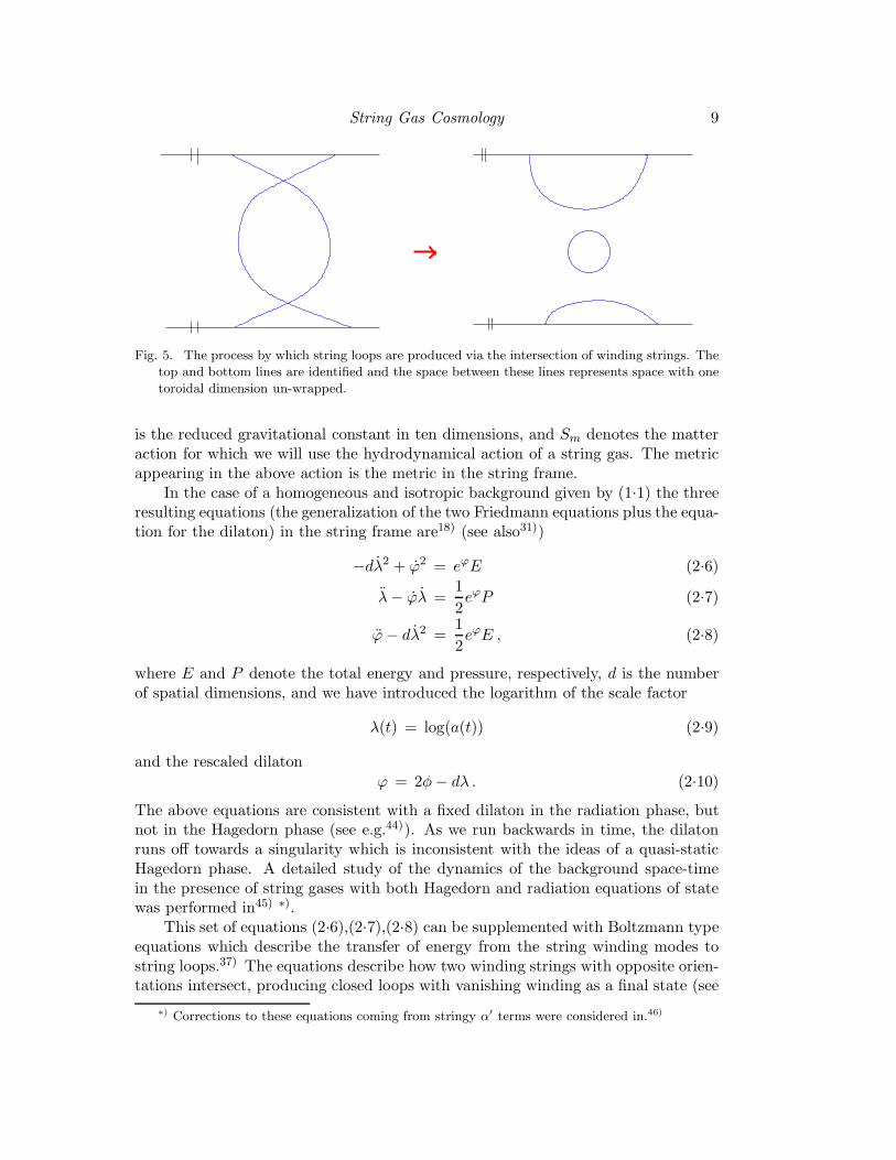
The transition between the quasi-static Hagedorn phase and the radiation phaseat the time tR is a consequence of the annihilation of string winding modes into stringloops (see Figure 5). Since this process corresponds to the production of radiation,we denote this time by the same symbol as the time of reheating in inflationarycosmology. As pointed out in,17) this annihilation process only is possible in at

8 R. Brandenberger

a

tt Rp = 0 p = rho / 3

~ t1/2

Fig. 4. The dynamics of string gas cosmology. The vertical axis represents the scale factor of the

universe, the horizontal axis is time. Along the horizontal axis, the approximate equation of state

is also indicated. During the Hagedorn phase the pressure is negligible due to the cancellation

between the positive pressure of the momentum modes and the negative pressure of the winding

modes, after time tR the equation of state is that of a radiation-dominated universe.

most three large spatial dimensions. This is a simple dimension counting argument:string world sheets have measure zero intersection probability in more than fourlarge space-time dimensions. Hence, string gas cosmology may provide a naturalmechanism for explaining why there are exactly three large spatial dimensions. Thisargument was supported by numerical studies of string evolution in three and fourspatial dimensions35) (see also36)). The flow of energy from winding modes to stringloops can be modelled by effective Boltzmann equations37) analogous to those usedto describe the flow of energy between infinite cosmic strings and cosmic string loops(see e.g.38)–40) for reviews).

Several comments are in place concerning the above mechanism. First, in theanalysis of37) it was assumed that the string interaction rates were time-independent.If the dynamics of the Hagedorn phase is modelled by dilaton gravity, the dilatonis rapidly changing during the phase in which the string frame scale factor is static.As discussed in,41), 42) in this case the mechanism which tells us that exactly threespatial dimensions become macroscopic does not work. Another comment concernsthe isotropy of the three large dimensions. In contrast to the situation in Stan-dard cosmology, in string gas cosmology the anisotropy decreases in the expandingphase.43) Thus, there is a natural isotropization mechanism for the three large spatialdimensions.

At late times, the dynamics of string gas cosmology can be described by dilatongravity or - if the dilaton is fixed - by Einstein gravity. The dilaton gravity actioncoupled to string gas matter is

S =1

2κ2

∫

d10x√−ge−2φ

[

R+ 4∂µφ∂µφ]

+ Sm , (2.5)

where g is the determinant of the metric, R is the Ricci scalar, φ is the dilaton, κ

String Gas Cosmology 9

Fig. 5. The process by which string loops are produced via the intersection of winding strings. The

top and bottom lines are identified and the space between these lines represents space with one

toroidal dimension un-wrapped.

is the reduced gravitational constant in ten dimensions, and Sm denotes the matteraction for which we will use the hydrodynamical action of a string gas. The metricappearing in the above action is the metric in the string frame.

In the case of a homogeneous and isotropic background given by (1.1) the threeresulting equations (the generalization of the two Friedmann equations plus the equa-tion for the dilaton) in the string frame are18) (see also31))

−dλ2 + ϕ2 = eϕE (2.6)

λ− ϕλ =1

2eϕP (2.7)

ϕ− dλ2 =1

2eϕE , (2.8)

where E and P denote the total energy and pressure, respectively, d is the numberof spatial dimensions, and we have introduced the logarithm of the scale factor

λ(t) = log(a(t)) (2.9)

and the rescaled dilatonϕ = 2φ− dλ . (2.10)

The above equations are consistent with a fixed dilaton in the radiation phase, butnot in the Hagedorn phase (see e.g.44)). As we run backwards in time, the dilatonruns off towards a singularity which is inconsistent with the ideas of a quasi-staticHagedorn phase. A detailed study of the dynamics of the background space-timein the presence of string gases with both Hagedorn and radiation equations of statewas performed in45) ∗).

This set of equations (2.6),(2.7),(2.8) can be supplemented with Boltzmann typeequations which describe the transfer of energy from the string winding modes tostring loops.37) The equations describe how two winding strings with opposite orien-tations intersect, producing closed loops with vanishing winding as a final state (see

∗) Corrections to these equations coming from stringy α′ terms were considered in.46)

10 R. Brandenberger

Figure 5). First, we split the energy density in strings into the density in windingstrings

ρw(t) = ν(t)µt−2 , (2.11)

where µ is the string mass per unit length, and ν(t) is the number of strings perHubble volume, and into the density in string loops

ρl(t) = g(t)e−3(λ(t)−λ(t0 )) , (2.12)

where g(t) denotes the co-moving number density of loops, normalized at a referencetime t0. In terms of these variables, the equations describing the loop productionfrom the interaction of two winding strings are37)

dν

dt= 2ν

(

t−1 −H)

− c′ν2t−1 (2.13)

dg

dt= c′µt−3ν2e3

(

λ(t)−λ(t0))

(2.14)

where c′ is a constant, which is of order unity for cosmic strings but which dependson the dilaton in the case of fundamental strings.41), 42)

If the spatial size is large in the Hagedorn phase, not all winding strings willdisappear at the time tR. In fact, as is well known from the studies of cosmicstrings,38)–40) the above transfer equations (2.13),(2.14) lead to the existence of ascaling solution for cosmic superstrings according to which at any given time inthe radiation phase for t > tR, there will be a distribution of cosmic superstringscharacterized by a constant average number of winding strings crossing each Hubblevolume. A remnant distribution of cosmic superstrings at all late times is thus oneof the testable predictions of string gas cosmology.

§3. Moduli Stabilization in String Gas Cosmology

3.1. Principles

A major challenge in string cosmology is to stabilize all of the string moduli.Specifically, the sizes and shapes of the extra dimensions must be stabilized, and somust the dilaton. In string gas cosmology based on heterotic superstring theory, allof the size and shape moduli are fixed by the basic ingredients of the model, namelythe presence of string states with both momentum and winding modes.

The stabilization of the size moduli was considered in,47)–50) that of the shapemoduli in51), 52) (see53) for a review). The basic principle is the following: in a stringgas containing both momentum and winding modes, the winding modes will preventexpansion since their energies increase with R whereas the momentum modes willprevent contraction since their energies scale as 1/R. Thus, on energetic grounds,there is a preferred value for the size of the extra dimensions, namely R = 1 in stringunits. In heterotic string theory, there are enhanced symmetry states which containboth momentum and winding quantum numbers and which are massless at the self-dual radius. These are the lowest energy states near the self-dual radius and hencedominate the thermodynamic partition function. These states act as radiation from

String Gas Cosmology 11

the point of view of our three large dimensions, and are hence phenomenologicallyacceptable at late times.49) The role of these states for moduli stabilization wasstressed in a more general context in.54)–56)

It turns out that the shape moduli are also stabilized by the presence of the en-hanced symmetry states, without requiring any additional inputs. The only moduluswhich requires additional input for its stabilization is the dilaton (the problem ofsimultaneously stabilizing both the dilaton and the radion in the context of dilatongravity coupled to perturbative string theory states was discussed in detail in57)).

3.2. Stabilization of Geometrical Moduli

The stabilization of the geometrical moduli at late times can be analyzed inthe context of dilaton gravity (the discussion in this subsection is close to the onegiven in53)). We use the following ansatz for an anisotropic metric with scale factora(t) = exp(λ(t)) for the three large dimensions and corresponding scale factor b(t) =exp(ν(t)) for the internal dimensions (considered here to be isotropic):

ds2 = dt2 − e2λdx2 − e2νdy2 , (3.1)

where x are the coordinates of the three large dimensions and y the coordinates ofthe internal dimensions.

The variational equations of motion for λ(t), ν(t) and φ(t) which follow fromthe dilaton gravity action are47)

−3λ− 3λ2 − 6ν − 6ν2 + 2φ =1

2e2φρ (3.2)

λ+ 3λ2 + 6λν − 2λφ =1

2e2φpλ (3.3)

ν + 6ν2 + 3λν − 2νφ =1

2e2φpν (3.4)

−4φ+ 4φ2 − 12λφ− 24νλ+ 3λ

+6λ2 + 6ν + 21ν2 + 18λν = 0 . (3.5)

where ρ is the energy density and pλ and pν are the pressure densities in the largeand the internal directions, respectively.

Let us now consider a superposition of several string gases, one with momentumnumber M3 about the three large dimensions, one with momentum number M6

about the six internal dimensions, and a further one with winding number N6 aboutthe internal dimensions. Note that there are no winding modes about the largedimensions (N3 = 0), either because they have already annihilated by the mechanismdiscussed in the previous section, or they were never present in the initial conditions.In this case, the energy E and the total pressures Pλ and Pν are given by

E = µ[

3M3e−λ + 6M6e

−ν + 6N6eν]

(3.6)

Pλ = µM3e−λ (3.7)

Pν = µ[

−N6eν +M6e

−ν]

, (3.8)

where µ is the string mass per unit length. Below, we will consider a more realistic

12 R. Brandenberger

string gas, a gas made up of string states which have momentum, winding and oscilla-tory quantum numbers together. The states considered here are massive, and wouldnot be expected to dominate the thermodynamical partition function if there arestates which are massless. However, for the purpose of studying radion stabilizationin the string frame, the use of the above naive string gas is sufficient.

We are interested in the symmetric case M6 = N6 In this case, it follows from(3.8) that the equation of motion for ν is a damped oscillator equation, with theminimum of the effective potential corresponding to the self-dual radius. The damp-ing is due to the expansion of the three large dimensions (the expansion of the threelarge dimensions is driven by the pressure from the momentum modes N3). Thus, wesee that the naive intuition that the competition of winding and momentum modesabout the compact directions stabilizes the radion degrees of freedom at the self-dualradius generalizes to this anisotropic setting.

However, in the context of dilaton gravity, the dilaton is rapidly evolving in theHagedorn phase. Thus, the Einstein frame metric is not static even if the string framemetric is (see e.g.58)). The key question is whether the radion remains stabilized ifthe dilaton is fixed by hand (or by mechanisms discussed below). For a gas of stringsmade up of massive states such as considered above this is not the case. In Heteroticstring theory, there are enhanced symmetry states which are massless at the self-dualradius, hence dominate the thermodynamic partition function, and can stabilize theradion.49) In the following we will discuss this mechanism.

The equations of motion which arise from coupling string gas matter to theEinstein (as opposed to the dilaton gravity) action lead to - for an anisotropic metricof the form

ds2 = dt2 − a(t)2dx2 −6

∑

α=1

bα(t)2dy2α , (3.9)

where the yα are the internal coordinates - the following equation for the radion bα

bα +(

3H +6

∑

β=1,β 6=α

bβbβ

)

bα =∑

n,m

8πGµm,n√gǫm,n

S . (3.10)

The vector index pairs (m,n) label perturbative string states. Note that n and mare momentum and winding number six-vectors, one component for each internaldimension. Also, µm,n is the number density of string states with the momentumand winding number vector pair (m,n), ǫm,n is the energy of an individual (m,n)string, and g is the determinant of the metric. The source term S depends on thequantum numbers of the string gas, and the sum runs over all m and n. If thenumber of right-moving oscillator modes is given by N , then the source term forfixed m and n is

S =∑

α

(mα

bα

)2 −∑

α

n2αb

2α +

2

D − 1

[

(n, n) + (n,m) + 2(N − 1)]

, (3.11)

where (n, n) and (n,m) indicate scalar products relative to the metric of the internalspace. To obtain this equation, we have made use of the mass spectrum of string

String Gas Cosmology 13

states and of the level matching conditions. In the case of the bosonic superstring,the mass spectrum for fixed m,n,N and N , where N is the number of left-movingoscillator states, on a six-dimensional torus whose radii are given by bα is

m2 =∑

α

(mα

bα

)2 −∑

α

n2αb

2α + 2(N + N − 2) , (3.12)

and the level matching condition reads

N = (n,m) +N . (3.13)

There are modes which are massless at the self-dual radius bα = 1. One suchmode is the graviton with n = m = 0 and N = 1. The modes of interest to us aremodes which contain winding and momentum, namely

• N = 1, (m,m) = 1, (m,n) = −1 and (n, n) = 1;• N = 0, (m,m) = 1, (m,n) = 1 and (n, n) = 1;• N = 0 (m,m) = 2, (m,n) = 0 and (n, n) = 2.

The above discussion was in the context of bosonic string theory. Due to the presenceof the bosonic string theory tachyon, the above states are not the lowest energy statesfor bosonic string theory and hence do not dominate the thermodynamic partitionfunction. In Heterotic string theory, the tachyon is factored out of the spectrumby the GSO27) projection, but the states we discussed above survive. In contrast,in Type II string theory, our massless states are also factored out. Thus, in thefollowing we will restrict attention to Heterotic string theory.

In string theories which admit massless states (i.e. states which are massless atthe self-dual radius), these states will dominate the initial partition function. Thebackground dynamics will then also be dominated by these states. To understandthe effect of these strings, consider the equation of motion (3.10) with the sourceterm (3.11). The first two terms in the source term S correspond to an effectivepotential with a stable minimum at the self-dual radius. However, if the third termin the source S does not vanish at the self-dual radius, it will lead to a positivepotential which causes the radion to increase. Thus, a condition for the stabilizationof bα at the self-dual radius is that the third term in (3.11) vanishes at the self-dualradius. This is the case if and only if the string state is a massless mode.

The massless modes have other nice features which are explored in detail in.49)

They act as radiation from the point of view of our three large dimensions and hencedo not lead to a over-abundance problem. As our three spatial dimensions grow, thepotential which confines the radion becomes shallower. However, rather surprisingly,it turns out the the potential remains steep enough to avoid fifth force constraints.

Key to the success in simultaneously avoiding the moduli over-closure problemand evading fifth force constraints is the fact that the stabilization mechanism is anintrinsically stringy one. In the case of a naive effective field theory approach, boththe confining force and the over-density in the moduli field scale as V (ϕ), where V (ϕ)is the potential energy density of the field ϕ. In contrast, in the case of stabilizationby means of massless string modes, the energy density in the string modes (from thepoint of view of our three large dimensions) scales as p3, whereas the confining force

14 R. Brandenberger

scales as p−13 , where p3 is the momentum in the three large dimensions. Thus, for

small values of p3, one simultaneously gets a large confining force (thus satisfyingthe fifth force constraints) and a small energy density.49), 59)

In the presence of massless string states, the shape moduli also can be stabilized,at least in the simple toroidal backgrounds considered so far.51) To study this issue,we consider a metric of the form

ds2 = dt2 − dx2 −Gmndymdyn , (3.14)

where the metric of the internal space (here for simplicity considered to be a two-dimensional torus) contains a shape modulus, the angle θ between the two cycles ofthe torus:

G11 = G22 = 1 (3.15)

and

G12 = G21 = sinθ , (3.16)

where θ = 0 corresponds to a rectangular torus. The ratio between the two toroidalradii is a second shape modulus. However, we already know that each radion indi-vidually is stabilized at the self-dual radius. Thus, the shape modulus correspondingto the ratio of the toroidal radii is fixed, and the angle is the only shape moduluswhich has yet to be considered.

Combining the 00 and the 12 Einstein equations, we obtain a harmonic oscillatorequation for θ with θ = 0 as the stable fixed point.

θ + 8K−1/2e−2φθ = 0 , (3.17)

where K is a constant whose value depends on the quantum numbers of the stringgas. In the case of an expanding three-dimensional space we would have obtained anadditional damping term in the above equation of motion. We thus conclude thatthe shape modulus is dynamically stabilized at a value which maximizes the area tocircumference ratio.

3.3. Dilaton Stabilization

The only modulus which is not stabilized with the basic ingredients of string gascosmology alone is the dilaton. This situation should be compared to the problemswhich arise in the string theory-motivated approaches to obtaining inflation, wherea number of extra ingredients such as fluxes and non-perturbative effects have to beinvoked in order to stabilize the Kaehler and complex structure moduli (see e.g.60)

for a review).In string gas cosmology, extra inputs are needed to stabilize the dilaton. One pos-

sibility is that two-loop effective potential effects can stabilize the dilaton.61) Therehave also been attempts to use extra stringy ingredients such as branes59), 62), 63) ora running tachyon33) to stabilize the dilaton.

The most conservative approach to late-time dilaton stabilization in string gascosmology,64) however, is to use one of the non-perturbative mechanisms which isalready widely used in the literature to fix moduli, namely gaugino condensation.65)

String Gas Cosmology 15

Gaugino condensation leads to a correction of the superpotentialW of the theory,from which the actual potential is derived. The change in the superpotential of thefour-dimensional theory is

W → W −Ae−1/g2, (3.18)

where g is the string coupling constant and A is a constant. The potential V canbe derived from the superpotential W and the Kaehler potential K via the standardformula

V =1

M2P

eK(

KABDAWDBW − 3|W |2)

, (3.19)

where the indices A and B run over all of the moduli fields, and the Kaehler covariantderivative is given by

DAW = ∂AW + (∂AK)W . (3.20)

Since the superpotential in our case is independent of the volume modulus, theexpression for the potential simplifies to

V =1

M2P

eKKabDaWDbW , (3.21)

where a and b now run only over the modulus

S = e−Φ + ia (3.22)

and the complex structure moduli (which we, however, do not include here). In theabove, Φ is the four-dimensional dilaton given by

Φ = 2φ− 6lnb , (3.23)

a is the axion, and MP is the four dimensional Planck mass.From the above, we see that the potential (3.19) depends both on the dilaton and

on the radion. It is important to verify that adding this potential to the theory canstabilize the dilaton without de-stabilizing the radion (which is fixed by the stringgas matter contributions described in the previous subsection). To investigate thisissue,64) we first need to lift the potential (3.19) to ten space-time dimensions. Theresult, after expanding about the minimum Φ0 of the potential, is

V (b, φ) =M16

10 V

4e−Φ0a2

0A2

(

a0 −3

2eΦ0

)2

e−2a0e−Φ0

×e−3φ/2(

b6e−2φ − e−Φ0

)2, (3.24)

where we have written the scale factor in the ten dimensional Einstein frame. Inthe above, V is the volume of the internal space, and M10 is the ten dimensionalPlanck mass which is given in terms of the volume of the internal space and the fourdimensional Planck mass by

M2P = M8

10V . (3.25)

Also, a0 is a constant which appears in the superpotential (see64) for details).

16 R. Brandenberger

The effects of gaugino condensation on dilaton and radion stabilization can nowbe analyzed in the following way:64) we start from the dilaton gravity action to whichwe add the potential (3.24). To this action we add the action of a gas of strings, asdone in (2.5). We work in the ten-dimensional Einstein frame (and thus have to re-scale the radion, the metric and the matter energy-momentum tensor accordingly).From this action we can derive the equations of motion for the dilaton, the radionand the scale factor of our four-dimensional space-time.

For fixed radion, it follows from (3.24) that the potential has a minimum for aspecific value of the dilaton. From the considerations of the previous subsection weknow that stringy matter selects a preferred value of the radion, the self-dual radius.To demonstrate that the addition of the gaugino potential can stabilize the dilatonwithout de-stabilizing the radion we expand the equations of motion about the valueof the radion corresponding to the self-dual radius and the value of the dilaton forwhich the potential (3.24) is minimized for the chosen value of the radion. We haveshown64) that this is a stable fixed point of the dynamical system. Thus, we haveshown with the addition of gaugino condensation, in string gas cosmology all of themoduli are fixed.

§4. String Gas Cosmology and Structure Formation

4.1. Overview

At the outset of this section, let us recall the mechanism by which inflationarycosmology leads to the possibility of a causal generation mechanism for cosmologicalfluctuations which yields an almost scale-invariant spectrum of perturbations. Thespace-time diagram of inflationary cosmology is sketched in Figure 1. In this figure,the vertical axis represents time, the horizontal axis space (physical as opposed toco-moving coordinates). The period between times ti and tR corresponds to theinflationary phase (assumed in the figure to be characterized by almost exponentialexpansion of space).

During the period of inflation, the Hubble radius

lH(t) =a

a(4.1)

is approximately constant. In contrast, the physical length of a fixed co-moving scale(labelled by k in the figure) is expanding exponentially. In this way, in inflationarycosmology scales which have microscopic sub-Hubble wavelengths at the beginningof inflation are red-shifted to become super-Hubble-scale fluctuations at the end ofthe period of inflation. After inflation, the Hubble radius increases linearly in time,faster than the physical wavelength corresponding to a fixed co-moving scale. Thus,scales re-enter the Hubble radius at late times.

The Hubble radius is crucial for the question of generation of fluctuations forthe following reason: If we consider perturbations with wavelengths smaller than theHubble radius, their evolution is dominated by micro-physics which causes them tooscillate. This is best illustrated by considering the Klein-Gordon equation for a free

String Gas Cosmology 17

scalar field ϕ in an expanding universe. In Fourier space, the equation is

ϕ+ 3Hϕ+ k2pϕ = 0 , (4.2)

where kp is the physical wavenumber. On sub-Hubble scales kp > H, the Hubbledamping term in the above equation is sub-dominant, and the micro-physics termk2

pϕ leads to oscillations of the field. In contrast, on super-Hubble scale kp < H, itis the last term on the left-hand side of (4.2) which is negligible, and it then followsthat the fluctuations are frozen in.

Thus, if we want to generate primordial cosmological fluctuations by causalphysics, the scale of the fluctuations needs to be sub-Hubble ∗). In inflationarycosmology, it is the accelerated expansion of space which enables the scale of inho-mogeneities on current cosmological scales to be sub-Hubble at early times, and thusleads to the possibility of a causal generation mechanism for fluctuations.

Since inflation red-shifts any classical fluctuations which might have been presentat the beginning of the inflationary phase, fluctuations in inflationary cosmology aregenerated by quantum vacuum perturbations. The fluctuations begin in their quan-tum vacuum state at the onset of inflation. Once the wavelength exceeds the Hubbleradius, squeezing of the wave-function of the fluctuations sets in (see12), 13)). Thissqueezing plus the de-coherence of the fluctuations due to the interaction betweenshort and long wavelength modes generated by the intrinsic non-linearities in boththe gravitational and matter sectors of the theory (see66)–68) for recent discussionsof this aspect and references to previous work) lead to the classicalization of thefluctuations on super-Hubble scales.

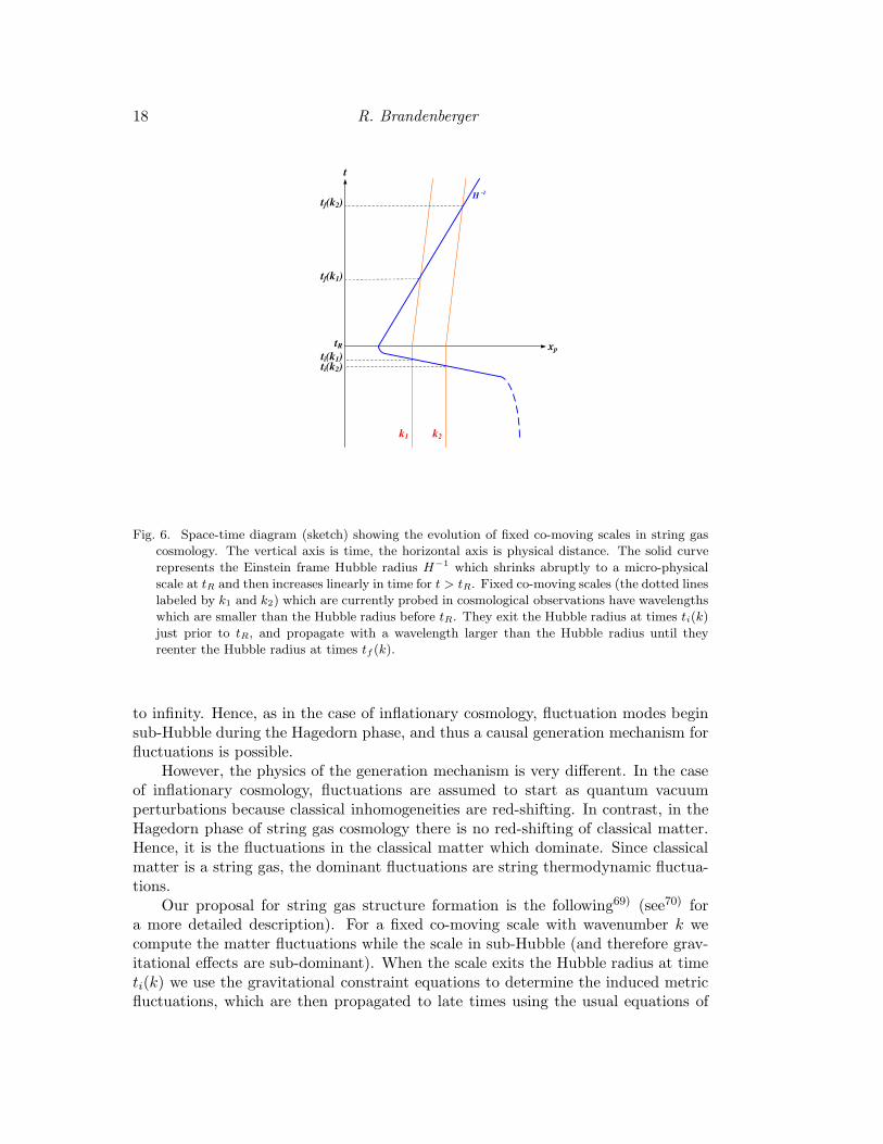
Let us now turn to the cosmological background of string gas cosmology rep-resented in Figure 4. This string gas cosmology background yields the space-timediagram sketched in Figure 6. As in Figure 1, the vertical axis is time and the hor-izontal axis denotes the physical distance. For times t < tR, we are in the staticHagedorn phase and the Hubble radius is infinite. For t > tR, the Einstein frameHubble radius is expanding as in standard cosmology. The time tR is when thestring winding modes begin to decay into string loops, and the scale factor starts toincrease, leading to the transition to the radiation phase of standard cosmology.

Let us now compare the evolution of the physical wavelength corresponding toa fixed co-moving scale with that of the Einstein frame Hubble radius H−1(t). Theevolution of scales in string gas cosmology is identical to the evolution in standardand in inflationary cosmology for t > tR. If we follow the physical wavelength of theco-moving scale which corresponds to the current Hubble radius back to the timetR, then - taking the Hagedorn temperature to be of the order 1016 GeV - we obtaina length of about 1 mm. Compared to the string scale and the Planck scale, this isa scale in the far infrared.

The physical wavelength is constant in the Hagedorn phase since space is static.But, as we enter the Hagedorn phase going back in time, the Hubble radius diverges

∗) There is, however, a loophole in this argument: the formation of topological defects during a

cosmological phase transition can lead to non-random entropy fluctuations on super-Hubble scales

which induce cosmological perturbations in the late universe.38)–40)

18 R. Brandenberger

H-1

k2k1

tR

tf(k2)

tf(k1)

ti(k1)ti(k2)

xp

t

Fig. 6. Space-time diagram (sketch) showing the evolution of fixed co-moving scales in string gas

cosmology. The vertical axis is time, the horizontal axis is physical distance. The solid curve

represents the Einstein frame Hubble radius H−1 which shrinks abruptly to a micro-physical

scale at tR and then increases linearly in time for t > tR. Fixed co-moving scales (the dotted lines

labeled by k1 and k2) which are currently probed in cosmological observations have wavelengths

which are smaller than the Hubble radius before tR. They exit the Hubble radius at times ti(k)

just prior to tR, and propagate with a wavelength larger than the Hubble radius until they

reenter the Hubble radius at times tf (k).

to infinity. Hence, as in the case of inflationary cosmology, fluctuation modes beginsub-Hubble during the Hagedorn phase, and thus a causal generation mechanism forfluctuations is possible.

However, the physics of the generation mechanism is very different. In the caseof inflationary cosmology, fluctuations are assumed to start as quantum vacuumperturbations because classical inhomogeneities are red-shifting. In contrast, in theHagedorn phase of string gas cosmology there is no red-shifting of classical matter.Hence, it is the fluctuations in the classical matter which dominate. Since classicalmatter is a string gas, the dominant fluctuations are string thermodynamic fluctua-tions.

Our proposal for string gas structure formation is the following69) (see70) fora more detailed description). For a fixed co-moving scale with wavenumber k wecompute the matter fluctuations while the scale in sub-Hubble (and therefore grav-itational effects are sub-dominant). When the scale exits the Hubble radius at timeti(k) we use the gravitational constraint equations to determine the induced metricfluctuations, which are then propagated to late times using the usual equations of

String Gas Cosmology 19

gravitational perturbation theory. Since the scales we are interested in are in the farinfrared, we use the Einstein constraint equations for fluctuations.

4.2. String Thermodynamics

The thermodynamics of a gas of strings was worked out some time ago ∗). Wewill consider our three spatial dimensions to be compact, admitting stable windingmodes. Specifically, we will take space to be a three-dimensional torus. In this case,the string gas specific heat is positive, and string thermodynamics is well-defined,and was discussed in detail in75) (see also76)–79)). What follows is a summary alongthe lines of.70)

The starting point for our considerations is the free energy F of a string gas inthermal equilibrium

F = − 1

βlnZ , (4.3)

where β is the inverse temperature and the canonical partition function Z is givenby

Z =∑

s

e−β√−g00H(s) , (4.4)

where the sum runs over the states s of the string gas, and H(s) is the energy of thestate. The action S of the string gas is given in terms of the free energy F via

S =

∫

dt√−g00F [gij , β] . (4.5)

Note that the free energy depends on the spatial components of the metric becausethe energy of the individual string states does. The energy-momentum tensor T µν

of the string gas is determined by varying the action with respect to the metric:

T µν =2√−g

δS

δgµν. (4.6)

Consider now the thermal expectation value

〈T µν〉 =

1

Z

∑

s

T µν(s)e−β

√−g00H(s) , (4.7)

where T µν(s) and H(s) are the energy momentum tensor and the energy of the state

labeled by s, respectively. Making use of (4.6) and (4.5) we immediately find that

T µν(s) = 2

gµλ

√−gδ

δgλµ[−√−g00H(s)] , (4.8)

and hence

〈T µν〉 = 2

gµλ

√−gδ lnZ

δgνλ. (4.9)

∗) The initial discussions of the thermodynamics of strings were given in.24), 71) More de-

tailed studies were performed after the first explosion of interest in superstring theory in the early

1980’s.72) For some studies of string statistical mechanics particularly relevant to string gas cosmol-

ogy see.73), 74)

20 R. Brandenberger

To extract the fluctuation tensor of Tµν for long wavelength modes, we take oneadditional variational derivative of (4.9), using (4.7) to obtain

〈T µνT

σλ〉 − 〈T µ

ν〉〈T σλ〉 = 2

gµα

√−g∂

∂gαν

(

gσδ

√−g∂ lnZ

∂gδλ

)

+2gσα

√−g∂

∂gαλ

(

Gµδ

√−g∂ lnZ

∂gδν

)

. (4.10)

As we will see below, the scalar metric fluctuations are determined by the energydensity correlation function

C0000 = 〈δρ2〉 = 〈ρ2〉 − 〈ρ〉2 . (4.11)

We will read off the result from the expression (4.10) evaluated for µ = ν = σ =λ = 0. The derivative with respect to g00 can be expressed in terms of the derivativewith respect to β. After a couple of steps of algebra we obtain

C0000 = − 1

R6

∂

∂β

(

F + β∂F

∂β

)

=T 2

R6CV . (4.12)

where

CV = (∂E/∂T )|V , (4.13)

is the specific heat, and

E ≡ F + β

(

∂F

∂β

)

, (4.14)

is the internal energy. Also, V = R3 is the volume of the three compact but largespatial dimensions.

The gravitational waves are determined by the off-diagonal spatial componentsof the correlation function tensor, i.e.

Cijij = 〈δT i

j2〉 = 〈T i

j2〉 − 〈T i

j〉2 , (4.15)

with i 6= j.Our aim is to calculate the fluctuations of the energy-momentum tensor on

various length scales R. For each value of R, we will consider string thermodynamicsin a box in which all edge lengths are R. From (4.10) it is obvious that in orderto have non-vanishing off-diagonal spatial correlation functions, we must consisted atorus with its shape moduli turned on. Let us focus on the x− y component of thecorrelation function. We will consider the spatial part of the metric to be

ds2 = R2dθ2x + 2ǫR2dθxdθy +R2dθ2

y (4.16)

with ǫ ≪ 1. The spatial coordinates θi run over a fixed interval, e.g. [0, 2π]), Thegeneralization of the spatial part of the metric to three dimensions is obvious. Atthe end of the computations, we will set ǫ = 0.

String Gas Cosmology 21

From the form of (4.10), it follows that all space-space correlation function tensorelements are of the same order of the magnitude, namely

Cijij =

1

βR3

∂

∂ lnR

(

− 1

R3

∂F

∂ lnR

)

=1

βR2

∂p

∂R, (4.17)

where the string pressure is given by

p ≡ − 1

V

(

∂F

∂ lnR

)

= T

(

∂S

∂V

)

E

. (4.18)

In the following, we will compute the two correlation functions (4.12) and (4.17)using tools from string statistical mechanics. Specifically, we will be following thediscussion in.75) The starting point is the formula

S(E,R) = lnΩ(E,R) (4.19)

for the entropy in terms of Ω(E,R), the density of states. The density of states of agas of closed strings on a large three-dimensional torus (with the radii of all internaldimensions at the string scale) was calculated in75) (see also80)) and is given by

Ω(E,R) ≃ βHeβHE+nHV [1 + δΩ(1)(E,R)] , (4.20)

where δΩ(1) comes from the contribution to the density of states (when writing thedensity of states as an inverse Laplace transform of Z(β), which involves integrationover β) from the closest singularity point β1 to βH = (1/TH ) in the complex β plane.Note that β1 < βH , and β1 is real. From75), 80) we have

δΩ(1)(E,R) = −(βHE)5

5!e−(βH−β1)(E−ρHV ) . (4.21)

In the above, nH is a (constant) number density of order l−3s and ρH is the ‘Hagedorn

Energy density’ of the order l−4s , and

βH − β1 ∼

(l3s/R2) , for R≫ ls ,

(R2/ls) , for R≪ ls .(4.22)

To ensure the validity of Eq. (4.20) we demand that

−δΩ(1) ≪ 1 (4.23)

by assuming ρ ≡ (E/V ) ≫ ρH , which corresponds to being in a state in which wind-ing modes and oscillatory modes can be excited and we expect important deviationsfrom point particle thermodynamics.

Combining the above results, we find that the entropy of the string gas in theHagedorn phase is given by

S(E,R) ≃ βHE + nHV + ln[

1 + δΩ(1)

]

, (4.24)

22 R. Brandenberger

and therefore the temperature T (E,R) ≡ [(∂S/∂E)V ]−1 will be

T ≃(

βH +∂δΩ(1)/∂E

1 + δΩ(1)

)−1

≃ TH

(

1 +βH − β1

βHδΩ(1)

)

. (4.25)

In the above, we have dropped a term which is negligible since E(βH − β1) ≫ 1 (see(4.23)). Using this relation, we can express δΩ(1) in terms of T and R via

l3sδΩ(1) ≃ −R2

TH

(

1 − T

TH

)

. (4.26)

In addition, we find

E ≃ l−3s R2 ln

[

ℓ3sT

R2(1 − T/TH)

]

. (4.27)

Note that to ensure that |δΩ(1)| ≪ 1 and E ≫ ρHR3, one should demand

(1 − T/TH)R2l−2s ≪ 1 . (4.28)

The results (4.24) and (4.26) now allow us to compute the correlation functions(4.12) and (4.17). We first compute the energy correlation function (4.12). Makinguse of (4.27), it follows from (4.13) that

CV ≈ R2/l3sT (1 − T/TH)

, (4.29)

from which we get

C0000 = 〈δρ2〉 ≃ T

l3s(1 − T/TH)

1

R4. (4.30)

Note that the factor (1−T/TH) in the denominator will turn out to be responsible forgiving the spectrum a slight red tilt. It comes from the differentiation with respectto T .

Next we evaluate (4.18). From the definition of the pressure it follows that (tolinear order in δΩ(1))

p = nHT + T∂

∂VδΩ(1) , (4.31)

where the final partial derivative is to be taken at constant energy. In taking thispartial derivative, we insert the expression (4.26) for δΩ(1) and must keep carefulaccount of the fact that βH −β1 depends on the radius R. In evaluating the resultingterms, we keep only the one which dominates at high energy density. It is the termwhich comes from differentiating the factor βH − β1. This differentiation bringsdown a factor of E, which is then substituted by means of (4.27), thus introducinga logarithmic factor in the final result for the pressure. We obtain

p(E,R) ≈ nHTH − 2

3

(1 − T/TH)

l3sRln

[

l3sT

R2(1 − T/TH)

]

, (4.32)

String Gas Cosmology 23

which immediately yields

Cijij ≃ T (1 − T/TH)

l3sR4

ln2

[

R2

l2s(1 − T/TH)

]

. (4.33)

Note that since no temperature derivative is taken, the factor (1 − T/TH) remainsin the numerator. This is one of the two facts which will lead to the slight blue tiltof the spectrum of gravitational waves. The second factor contributing to the slightblue tilt is the explicit factor of R2 in the logarithm. Because of (4.28), we are onthe large k side of the zero of the logarithm. Hence, the greater the value of k, thelarger the absolute value of the logarithmic factor.

4.3. Spectrum of Cosmological Fluctuations

We write the metric including cosmological perturbations (scalar metric fluctu-ations) and gravitational waves in the following form:

ds2 = a2(η)

(1 + 2Φ)dη2 − [(1 − 2Φ)δij + hij ]dxidxj

. (4.34)

In the above, we have used conformal time η which is related to the physical time tvia

dt = a(t)dη . (4.35)

We have fixed the gauge (i.e. coordinate) freedom for the scalar metric perturbationsby adopting the longitudinal gauge in terms of which the metric is diagonal. Further-more, we have taken matter to be free of anisotropic stress (otherwise there wouldbe two scalar metric degrees of freedom instead of the single function Φ(x, t)). Thespatial tensor hij(x, t) is transverse and traceless and represents the gravitationalwaves.

Note that in contrast to the case of slow-roll inflation, scalar metric fluctuationsand gravitational waves are generated by matter at the same order in cosmologi-cal perturbation theory. This could lead to the expectation that the amplitude ofgravitational waves in string gas cosmology could be generically larger than in in-flationary cosmology. This expectation, however, is not realized81) since there is adifferent mechanism which suppresses the gravitational waves relative to the den-sity perturbations (namely the fact that the gravitational wave amplitude is set bythe amplitude of the pressure, and the pressure is suppressed relative to the energydensity in the Hagedorn phase).

Assuming that the fluctuations are described by the perturbed Einstein equa-tions (they are not if the dilaton is not fixed44), 82)), then the spectra of cosmologicalperturbations Φ and gravitational waves h are given by the energy-momentum fluc-tuations in the following way70)

〈|Φ(k)|2〉 = 16π2G2k−4〈δT 00(k)δT

00(k)〉 , (4.36)

where the pointed brackets indicate expectation values, and

〈|h(k)|2〉 = 16π2G2k−4〈δT ij(k)δT

ij(k)〉 , (4.37)

24 R. Brandenberger

where on the right hand side of (4.37) we mean the average over the correlationfunctions with i 6= j, and h is the amplitude of the gravitational waves ∗).

Let us now use (4.36) to determine the spectrum of scalar metric fluctuations.We first calculate the root mean square energy density fluctuations in a sphere ofradius R = k−1. For a system in thermal equilibrium they are given by the specificheat capacity CV via (see (4.12)

〈δρ2〉 =T 2

R6CV . (4.38)

From the previous subsection we know that the specific heat of a gas of closed stringson a torus of radius R is (see 4.29)

CV ≈ 2R2/ℓ3

T (1 − T/TH). (4.39)

Hence, the power spectrum P (k) of scalar metric fluctuations can be evaluated asfollows

PΦ(k) ≡ 1

2π2k3|Φ(k)|2 (4.40)

= 8G2k−1 < |δρ(k)|2 > .

= 8G2k2 < (δM)2 >R

= 8G2k−4 < (δρ)2 >R

= 8G2 T

ℓ3s

1

1 − T/TH,

where in the first step we have used (4.36) to replace the expectation value of |Φ(k)|2in terms of the correlation function of the energy density, and in the second step wehave made the transition to position space

The first conclusion from the result (4.40) is that the spectrum is approximatelyscale-invariant (P (k) is independent of k). It is the ‘holographic’ scaling CV (R) ∼ R2

which is responsible for the overall scale-invariance of the spectrum of cosmologicalperturbations. However, there is a small k dependence which comes from the factthat in the above equation for a scale k the temperature T is to be evaluated at thetime ti(k). Thus, the factor (1− T/TH) in the denominator is responsible for givingthe spectrum a slight dependence on k. Since the temperature slightly decreases astime increases at the end of the Hagedorn phase, shorter wavelengths for which ti(k)occurs later obtain a smaller amplitude. Thus, the spectrum has a slight red tilt.

4.4. Spectrum of Gravitational Waves

As discovered in,81) the spectrum of gravitational waves is also nearly scaleinvariant. However, in the expression for the spectrum of gravitational waves thefactor (1 − T/TH) appears in the numerator, thus leading to a slight blue tilt in

∗) The gravitational wave tensor hij can be written as the amplitude h multiplied by a constant

polarization tensor.

String Gas Cosmology 25

the spectrum. This is a prediction with which the cosmological effects of string gascosmology can be distinguished from those of inflationary cosmology, where quitegenerically a slight red tilt for gravitational waves results. The physical reason isthat large scales exit the Hubble radius earlier when the pressure and hence also theoff-diagonal spatial components of Tµν are closer to zero.

Let us analyze this issue in a bit more detail and estimate the dimensionlesspower spectrum of gravitational waves. First, we make some general comments. Inslow-roll inflation, to leading order in perturbation theory matter fluctuations do notcouple to tensor modes. This is due to the fact that the matter background fieldis slowly evolving in time and the leading order gravitational fluctuations are linearin the matter fluctuations. In our case, the background is not evolving (at leastat the level of our computations), and hence the dominant metric fluctuations arequadratic in the matter field fluctuations. At this level, matter fluctuations induceboth scalar and tensor metric fluctuations. Based on this consideration we mightexpect that in our string gas cosmology scenario, the ratio of tensor to scalar metricfluctuations will be larger than in simple slow-roll inflationary models. However,since the amplitude h of the gravitational waves is proportional to the pressure, andthe pressure is suppressed in the Hagedorn phase, the amplitude of the gravitationalwaves will also be small in string gas cosmology.

The method for calculating the spectrum of gravitational waves is similar to theprocedure outlined in the last section for scalar metric fluctuations. For a modewith fixed co-moving wavenumber k, we compute the correlation function of the off-diagonal spatial elements of the string gas energy-momentum tensor at the time ti(k)when the mode exits the Hubble radius and use (4.37) to infer the amplitude of thepower spectrum of gravitational waves at that time. We then follow the evolutionof the gravitational wave power spectrum on super-Hubble scales for t > ti(k) usingthe equations of general relativistic perturbation theory.

The power spectrum of the tensor modes is given by (4.37):

Ph(k) = 16π2G2k−4k3〈δT ij(k)δT

ij(k)〉 (4.41)

for i 6= j. Note that the k3 factor multiplying the momentum space correlationfunction of T i

j gives the position space correlation function, namely the root meansquare fluctuation of T i

j in a region of radius R = k−1 (the reader who is skepticalabout this point is invited to check that the dimensions work out properly). Thus,

Ph(k) = 16π2G2k−4Cijij(R) . (4.42)

The correlation function Cijij on the right hand side of the above equation was

computed earlier (in the subsection on string thermodynamics). Inserting the result(4.33) into (4.41) we obtain

Ph(k) ∼ 16π2G2T

l3s(1 − T/TH) ln2

[

1

l2sk2(1 − T/TH)

]

, (4.43)

which, for temperatures close to the Hagedorn value reduces to

Ph(k) ∼(

lP l

ls

)4

(1 − T/TH) ln2

[

1

l2sk2(1 − T/TH)

]

. (4.44)

26 R. Brandenberger

This shows that the spectrum of tensor modes is - to a first approximation, namelyneglecting the logarithmic factor and neglecting the k-dependence of T (ti(k)) - scale-invariant. The corrections to scale-invariance will be discussed at the end of thissubsection.

On super-Hubble scales, the amplitude h of the gravitational waves is constant.The wave oscillations freeze out when the wavelength of the mode crosses the Hubbleradius. As in the case of scalar metric fluctuations, the waves are squeezed. Whereasthe wave amplitude remains constant, its time derivative decreases. Another way tosee this squeezing is to change variables to

ψ(η,x) = a(η)h(η,x) (4.45)

in terms of which the action has canonical kinetic term. The action in terms of ψbecomes

S =1

2

∫

d4x

(

ψ′2 − ψ,iψ,i +a′′

aψ2

)

(4.46)

from which it immediately follows that on super-Hubble scales ψ ∼ a. This is thesqueezing of gravitational waves.83)

Since there is no k-dependence in the squeezing factor, the scale-invariance ofthe spectrum at the end of the Hagedorn phase will lead to a scale-invariance of thespectrum at late times.

Note that in the case of string gas cosmology, the squeezing factor z(η) does notdiffer substantially from the squeezing factor a(η) for gravitational waves. In thecase of inflationary cosmology, z(η) and a(η) differ greatly during reheating, leadingto a much larger squeezing for scalar metric fluctuations, and hence to a suppressedtensor to scalar ratio of fluctuations. In the case of string gas cosmology, there is nodifference in squeezing between the scalar and the tensor modes.

Let us return to the discussion of the spectrum of gravitational waves. Theresult for the power spectrum is given in (4.44), and we mentioned that to a firstapproximation this corresponds to a scale-invariant spectrum. As realized in,81) thelogarithmic term and the k-dependence of T (ti(k)) both lead to a small blue-tilt of thespectrum. This feature is characteristic of our scenario and cannot be reproducedin inflationary models. In inflationary models, the amplitude of the gravitationalwaves is set by the Hubble constant H. The Hubble constant cannot increase duringinflation, and hence no blue tilt of the gravitational wave spectrum is possible.

To study the tilt of the tensor spectrum, we first have to keep in mind that ourcalculations are only valid in the range (4.28), i.e. to the large k side of the zero ofthe logarithm. Thus, in the range of validity of our analysis, the logarithmic factorcontributes an explicit blue tilt of the spectrum. The second source of a blue tilt isthe factor 1 − T (ti(k))/TH multiplying the logarithmic term in (4.44). Since modeswith larger values of k exit the Hubble radius at slightly later times ti(k), when thetemperature T (ti(k)) is slightly lower, the factor will be larger.

A heuristic way of understanding the origin of the slight blue tilt in the spectrumof tensor modes is as follows. The closer we get to the Hagedorn temperature, themore the thermal bath is dominated by long string states, and thus the smaller thepressure will be compared to the pressure of a pure radiation bath. Since the pressure

String Gas Cosmology 27

terms (strictly speaking the anisotropic pressure terms) in the energy-momentumtensor are responsible for the tensor modes, we conclude that the smaller the valueof the wavenumber k (and thus the higher the temperature T (ti(k)) when the modeexits the Hubble radius, the lower the amplitude of the tensor modes. In contrast,the scalar modes are determined by the energy density, which increases at T (ti(k))as k decreases, leading to a slight red tilt.

4.5. Discussion

To summarize this section, we have seen that string gas cosmology provides amechanism alternative to the well-known inflationary one for generating an approx-imately scale-invariant spectrum of approximately adiabatic density fluctuations.The model predicts a slight red tilt of the spectrum (as is also obtained in manysimple inflationary models). However, as a prediction which distinguishes the modelfrom the inflationary universe scenario, it predicts a slight blue tilt of the spectrumof gravitational waves. Thus, a way to rule out the inflationary scenario would beto detect a stochastic background of gravitational waves at both very small wave-lengths (using direct detection experiments such as gravitational wave antennas) andon cosmological scales (using signatures in CMB temperature maps) and to infer ablue tilt from those measurements. The current limits on the magnitude of the bluetilt are not very strong84) but can be improved.

The scenario has one free parameter (the ratio of the string to the Planck length)and one free function (the k-dependence of the temperature T (ti(k)) - in principlecalculable if the dynamics of the exit from the Hagedorn phase were better known).There are five basic observables: the amplitudes of the scalar and tensor spectra,their tilts, and the amplitude of the jump in the CMB temperature maps producedby long straight cosmic superstrings via the Kaiser-Stebbins85) effect. Thus, thereare three consistency relations between the observables which allow the scenario tobe falsified.

An important point is that the thermal string gas fluctuations evolve for a longtime during the radiation phase outside the Hubble radius. Like in inflationarycosmology, this leads to the squeezing of fluctuations which is responsible for theacoustic oscillations in the angular power spectrum of CMB anisotropies (see e.g.70)

for a more detailed discussion of this point). Note that the situation is completelydifferent from that in topological defect models of structure formation, where thecurvature perturbations are constantly seeded from the defect sources at late times,and which hence does not lead to the oscillations in the angular power spectrum ofthe CMB.

The non-Gaussianities induced by the thermal gas of strings are large on mi-croscopic scale, but Poisson-suppressed on larger scales. The three point correlationfunction produced by a string gas and the related non-Gaussianity parameter canbe calculated86) from the same starting point of string thermodynamics describedearlier in this section.

Note that the structure formation scenario discussed in this section relies onthree key assumptions - firstly the holographic scaling of the specific heat capacityCV (R) ∼ R2, secondly the applicability of the Einstein equations to describe metric

28 R. Brandenberger

fluctuations on infrared scales, and thirdly the existence of a phase like the Hagedornphase at the end of which the matter fluctuations seed metric perturbations (it maybe a phase only describable using a truly non-perturbative string theory or quantumgravity framework). For attempts to realize our basic structure formation scenarioin a different context see e.g.87)

Dilaton gravity does not provide a satisfactory framework to implement ourstructure formation scenario44), 82) and is unsatisfactory as a description of the Hage-dorn phase for other reasons mentioned earlier in this chapter. The criticisms ofstring gas cosmology in82), 88) are mostly problems which are specific to the attemptto use dilaton gravity as the background for string gas cosmology. There is a spe-cific background model in which all of the key assumptions discussed above arerealized, namely the ghost-free higher derivative gravity action of89) which yields anon-singular bouncing cosmology. If we add string gas matter to this action andadjust parameters of the model such that the bounce phase is long, then thermalstring fluctuations in the bounce phase yield a realization of our scenario.90)

§5. Conclusions

The string gas scenario is an approach to early universe cosmology based oncoupling a gas of strings to a classical background. It includes string degrees offreedom and string symmetries which are hard to implement in an effective fieldtheory approach.

The background of string gas cosmology is non-singular. The temperature neverexceeds the limiting Hagedorn temperature. If we start the evolution as a densegas of strings in a space in which all dimensions are string-scale tori, then there aredynamical arguments according to which only three of the spatial dimensions canbecome large.17) Thus, string gas cosmology yields the hope of understanding why- in the context of a theory with more than three spatial dimensions - exactly threeare large and visible to us.

If the Hagedorn phase (the phase during which the temperature is close to theHagedorn temperature and both the scale factor and the dilaton are static) is suffi-ciently long to establish thermal equilibrium on length scales of about 1 mm, thenstring gas cosmology can provide an alternative to cosmological inflation for explain-ing the origin of an almost scale-invariant spectrum of cosmological fluctuations.69)

A distinctive signature of the scenario is the slight blue tilt in the spectrum of grav-itational waves which is predicted.81)

The inflationary universe scenario has successes beyond the fact that it suc-cessfully predicted a scale-invariant spectrum of fluctuations - it also explains why,starting from a hot Planck scale space, an extremely low entropy state - one canobtain a universe which is large enough and contains enough entropy to correspondto our observed universe. In addition, it explains the observed spatial flatness. How-ever, if the Hagedorn phase of string gas cosmology is realized as a long bouncephase in a universe which starts out large and cold, then the horizon, flatness, sizeand entropy problems do not arise.

A serious concern for the current realization of string gas cosmology, however, is

String Gas Cosmology 29

the gravitational Jeans instability problem. This problem was first raised in.91) Inthe context of dilaton gravity, it can be shown92) that gravitational fluctuations donot grow. However, dilaton gravity is not a consistent background for the Hagedornphase of string gas cosmology. One might hope that since the string states arerelativistic, the gravitational Jeans length will be comparable to the Hubble radius,as it is for a gas of regular radiation. However, a recent computation of the speed ofsound in string gas cosmology93) has shown that in a background space sufficientlylarge to evolve into our present universe the overall speed of sound is very small.Further work needs to be done on this issue. This is complicated by fact that stringthermodynamics is non-extensive (see e.g.94)), which leads to problems in using theusual thermodynamic intuition.

Note that the background space does not need to be toroidal. Crucial for stringgas cosmology to yield the predictions summarized above is the existence and stabil-ity (or quasi-stability) of string winding modes. Certain orbifolds95) have also beenshown to yield good backgrounds for string gas cosmology. Non-trivial one cycleswill ensure the existence and stability of string winding modes.

If the background space does not have have any non-trivial one-cycles, then itmight be possible to construct a cosmological scenario based on stable branes ratherthan strings. The cosmology of brane gases has been considered in.96) If there arestable winding strings, and if the string coupling constant is small such that thefundamental strings are lighter than branes, then19) it is the fundamental stringswhich will dominate the thermodynamics in the Hagedorn phase and which will bethe most important degrees of freedom for cosmology. However, if there are no stablewinding strings, then winding branes would become important.

It appears at the present time that Heterotic string theory is most suited forstring gas cosmology since this theory admits the enhanced symmetry states whichhave been shown to yield a very simple way to stabilize the size and shape moduliof the extra spatial dimensions. It will be interesting to study if string gas cosmol-ogy can be embedded into particular models of Heterotic string theory which yieldreasonable particle phenomenology.

The presentation we gave of string gas cosmology is based on minimal input.In particular, we did not include fluxes since we assume that the net fluxes shouldcancel for a situation with the most symmetric initial conditions. The role of fluxesin string gas cosmology has been studied in.97) Whereas the primary application ofstring gas cosmology will be to the cosmology of the very early universe, it is alsointeresting to consider applications of string gas cosmology to later time cosmology.The late time dynamics of string and brane gases has been considered in.98) Inparticular, in99) applications of string gases to the dark energy problem has beenconsidered (see also100)). String and brane gases have also been studied as a wayto obtain inflation101)–103) (see also104)), or as a way to obtain non-inflationary bulkexpansion which may provide a way to solve the size problem in string gas cosmologyif one starts with a spatial manifold of string scale in all directions.105)

Acknowledgements

I am grateful to all of my present and former collaborators with whom I have

30 R. Brandenberger

had the pleasure of working on string gas cosmology. For comments on the draftof this manuscript I wish to thank Nima Lashkari and Subodh Patil. This work issupported in part by an NSERC Discovery Grant and by funds from the CanadaResearch Chairs Program.

References

1) A. H. Guth, “The Inflationary Universe: A Possible Solution To The Horizon And Flat-ness Problems,” Phys. Rev. D 23, 347 (1981).

2) K. Sato, “First Order Phase Transition Of A Vacuum And Expansion Of The Universe,”Mon. Not. Roy. Astron. Soc. 195, 467 (1981).

3) A. A. Starobinsky, “A New Type Of Isotropic Cosmological Models Without Singularity,”Phys. Lett. B 91, 99 (1980).

4) R. Brout, F. Englert and E. Gunzig, “The Creation Of The Universe As A QuantumPhenomenon,” Annals Phys. 115, 78 (1978).

5) V. F. Mukhanov and G. V. Chibisov, “Quantum Fluctuation And ’Nonsingular’ Universe.(In Russian),” JETP Lett. 33, 532 (1981) [Pisma Zh. Eksp. Teor. Fiz. 33, 549 (1981)].

6) W. Press, “Spontaneous production of the Zel’dovich spectrum of cosmological fluctua-tions”, Phys. Scr. 21, 702 (1980).

7) A. A. Starobinsky, “Spectrum of relict gravitational radiation and the early state of theuniverse,” JETP Lett. 30, 682 (1979) [Pisma Zh. Eksp. Teor. Fiz. 30, 719 (1979)].

8) V. N. Lukash, “Production Of Phonons In An Isotropic Universe,” Sov. Phys. JETP 52,807 (1980) [Zh. Eksp. Teor. Fiz. 79, (1980)].

9) R. A. Sunyaev and Y. B. Zeldovich, “Small scale fluctuations of relic radiation,” Astro-phys. Space Sci. 7, 3 (1970).

10) C. B. Netterfield et al. [Boomerang Collaboration], “A measurement by BOOMERANGof multiple peaks in the angular power spectrum of the cosmic microwave background,”Astrophys. J. 571, 604 (2002) [arXiv:astro-ph/0104460].

11) C. L. Bennett et al., “First Year Wilkinson Microwave Anisotropy Probe (WMAP) Ob-servations: Preliminary Maps and Basic Results,” Astrophys. J. Suppl. 148, 1 (2003)[arXiv:astro-ph/0302207].

12) V. F. Mukhanov, H. A. Feldman and R. H. Brandenberger, “Theory Of Cosmological Per-turbations. Part 1. Classical Perturbations. Part 2. Quantum Theory Of Perturbations.Part 3. Extensions,” Phys. Rept. 215, 203 (1992).

13) R. H. Brandenberger, “Lectures on the theory of cosmological perturbations,” Lect. NotesPhys. 646, 127 (2004) [arXiv:hep-th/0306071].

14) A. Borde and A. Vilenkin, “Eternal inflation and the initial singularity,” Phys. Rev. Lett.72, 3305 (1994) [arXiv:gr-qc/9312022].

15) R. H. Brandenberger, [arXiv:hep-ph/9910410]. “Inflationary cosmology: Progress andproblems,”

16) R. H. Brandenberger and J. Martin, Mod. Phys. Lett. A 16, 999 (2001), [arXiv:astro-ph/0005432]; J. Martin and R. H. Brandenberger, Phys. Rev. D 63, 123501 (2001),[arXiv:hep-th/0005209].

17) R. H. Brandenberger and C. Vafa, “Superstrings In The Early Universe,” Nucl. Phys. B316, 391 (1989).

18) A. A. Tseytlin and C. Vafa, “Elements of string cosmology,” Nucl. Phys. B 372, 443(1992) [arXiv:hep-th/9109048].

19) S. Alexander, R. H. Brandenberger and D. Easson, “Brane gases in the early universe,”Phys. Rev. D 62, 103509 (2000) [arXiv:hep-th/0005212].

20) J. Kripfganz and H. Perlt, “Cosmological Impact Of Winding Strings,” Class. Quant.Grav. 5, 453 (1988).

21) E. Alvarez and M. A. R. Osorio, “Primordial Superstrings and the Origin of the Universe,”Int. J. Theor. Phys. 28, 949 (1989); N. Matsuo, “Very Eearly Universe Based on ClosedSuperstring Theories,” Prog. Theor. Phys. 77, 223 (1987).

22) R. H. Brandenberger, “Challenges for string gas cosmology,” arXiv:hep-th/0509099.23) T. Battefeld and S. Watson, “String gas cosmology,” Rev. Mod. Phys. 78, 435 (2006)

[arXiv:hep-th/0510022].

String Gas Cosmology 31

24) R. Hagedorn, “Statistical Thermodynamics Of Strong Interactions At High-Energies,”Nuovo Cim. Suppl. 3, 147 (1965).

25) S. Kalyana Rama, “Can string theory avoid cosmological singularities?,” Phys. Lett. B408, 91 (1997) [arXiv:hep-th/9701154].

26) D. A. Easson, “Towards a stringy resolution of the cosmological singularity,” Phys. Rev.D 68, 043514 (2003) [arXiv:hep-th/0304168].

27) J. Polchinski, String Theory, Vols. 1 and 2, (Cambridge Univ. Press, Cambridge, 1998).28) T. Boehm and R. Brandenberger, “On T-duality in brane gas cosmology,” JCAP 0306,

008 (2003) [arXiv:hep-th/0208188].29) K. Hotta, K. Kikkawa and H. Kunitomo, “Correlation between momentum modes and

winding modes in Brandenberger-Vafa’s string cosmological model,” Prog. Theor. Phys.98, 687 (1997) [arXiv:hep-th/9705099].

30) M. A. R. Osorio and M. A. Vazquez-Mozo, “A Cosmological Interpretation Of Duality,”Phys. Lett. B 320, 259 (1994) [arXiv:hep-th/9311080].

31) G. Veneziano, “Scale factor duality for classical and quantum strings,” Phys. Lett. B265, 287 (1991).

32) A. A. Tseytlin, “Dilaton, winding modes and cosmological solutions,” Class. Quant. Grav.9, 979 (1992) [arXiv:hep-th/9112004].

33) R. H. Brandenberger, A. R. Frey and S. Kanno, “Towards A Nonsingular Tachyonic BigCrunch,” Phys. Rev. D 76, 063502 (2007) [arXiv:0705.3265 [hep-th]].

34) S. Arapoglu, A. Karakci and A. Kaya, “S-duality in string gas cosmology,” Phys. Lett.B 645, 255 (2007) [arXiv:hep-th/0611193].

35) M. Sakellariadou, “Numerical Experiments in String Cosmology,” Nucl. Phys. B 468,319 (1996) [arXiv:hep-th/9511075].

36) G. B. Cleaver and P. J. Rosenthal, “String cosmology and the dimension of space-time,”Nucl. Phys. B 457, 621 (1995) [arXiv:hep-th/9402088].

37) R. Brandenberger, D. A. Easson and D. Kimberly, “Loitering phase in brane gas cosmol-ogy,” Nucl. Phys. B 623, 421 (2002) [arXiv:hep-th/0109165].

38) A. Vilenkin and E.P.S. Shellard, Cosmic Strings and other Topological Defects (Cam-bridge Univ. Press, Cambridge, 1994).

39) M. B. Hindmarsh and T. W. B. Kibble, “Cosmic strings,” Rept. Prog. Phys. 58, 477(1995) [arXiv:hep-ph/9411342].

40) R. H. Brandenberger, “Topological defects and structure formation,” Int. J. Mod. Phys.A 9, 2117 (1994) [arXiv:astro-ph/9310041].

41) R. Easther, B. R. Greene, M. G. Jackson and D. Kabat, “String windings in the earlyuniverse,” JCAP 0502, 009 (2005) [arXiv:hep-th/0409121].

42) R. Danos, A. R. Frey and A. Mazumdar, “Interaction rates in string gas cosmology,”Phys. Rev. D 70, 106010 (2004) [arXiv:hep-th/0409162].

43) S. Watson and R. H. Brandenberger, “Isotropization in brane gas cosmology,” Phys. Rev.D 67, 043510 (2003) [arXiv:hep-th/0207168].

44) R. H. Brandenberger et al., “More on the spectrum of perturbations in string gas cos-mology,” JCAP 0611, 009 (2006) [arXiv:hep-th/0608186].

45) B. A. Bassett, M. Borunda, M. Serone and S. Tsujikawa, “Aspects of string-gas cosmologyat finite temperature,” Phys. Rev. D 67, 123506 (2003) [arXiv:hep-th/0301180].

46) M. Borunda and L. Boubekeur, “The effect of alpha’ corrections in string gas cosmology,”JCAP 0610, 002 (2006) [arXiv:hep-th/0604085].

47) S. Watson and R. Brandenberger, “Stabilization of extra dimensions at tree level,” JCAP0311, 008 (2003) [arXiv:hep-th/0307044].

48) S. P. Patil and R. Brandenberger, “Radion stabilization by stringy effects in generalrelativity and dilaton gravity,” Phys. Rev. D 71, 103522 (2005) [arXiv:hep-th/0401037].

49) S. P. Patil and R. H. Brandenberger, “The cosmology of massless string modes,”arXiv:hep-th/0502069.

50) A. Kaya, “On winding branes and cosmological evolution of extra dimensions in stringtheory,” Class. Quant. Grav. 20, 4533 (2003) [arXiv:hep-th/0302118]; A. Kaya andT. Rador, “Wrapped branes and compact extra dimensions in cosmology,” Phys. Lett. B565, 19 (2003) [arXiv:hep-th/0301031]; A. Kaya, “Volume stabilization and accelerationin brane gas cosmology,” JCAP 0408, 014 (2004) [arXiv:hep-th/0405099]; S. Arapogluand A. Kaya, “D-brane gases and stabilization of extra dimensions in dilaton gravity,”

32 R. Brandenberger

Phys. Lett. B 603, 107 (2004) [arXiv:hep-th/0409094]; T. Rador, “Vibrating windingbranes, wrapping democracy and stabilization of extra dimensions in dilaton gravity,”JHEP 0506, 001 (2005) [arXiv:hep-th/0502039]; T. Rador, “Intersection democracy forwinding branes and stabilization of extra dimensions,” Phys. Lett. B 621, 176 (2005)[arXiv:hep-th/0501249]; T. Rador, “Stabilization of Extra Dimensions and The Dimen-sionality of the Observed Space,” Eur. Phys. J. C 49, 1083 (2007) [arXiv:hep-th/0504047];A. Chatrabhuti, “Target space duality and moduli stabilization in string gas cosmology,”Int. J. Mod. Phys. A 22, 165 (2007) [arXiv:hep-th/0602031]; J. Y. Kim, “Stabilizationof the extra dimensions in brane gas cosmology with bulk flux,” Phys. Lett. B 652,43 (2007) [arXiv:hep-th/0608131]; J. Y. Kim, “Radion effective potential in brane gascosmology,” arXiv:0804.0073 [hep-th].

51) R. Brandenberger, Y. K. Cheung and S. Watson, “Moduli stabilization with string gasesand fluxes,” JHEP 0605, 025 (2006) [arXiv:hep-th/0501032].

52) A. Kaya, “Brane gases and stabilization of shape moduli with momentum and windingstress,” Phys. Rev. D 72, 066006 (2005) [arXiv:hep-th/0504208].

53) R. H. Brandenberger, “Moduli stabilization in string gas cosmology,” Prog. Theor. Phys.Suppl. 163, 358 (2006) [arXiv:hep-th/0509159].

54) S. Watson, “Moduli stabilization with the string Higgs effect,” Phys. Rev. D 70, 066005(2004) [arXiv:hep-th/0404177]; S. Watson, “Stabilizing moduli with string cosmology,”arXiv:hep-th/0409281.

55) L. Kofman, A. Linde, X. Liu, A. Maloney, L. McAllister and E. Silverstein, “Beautyis attractive: Moduli trapping at enhanced symmetry points,” JHEP 0405, 030 (2004)[arXiv:hep-th/0403001].

56) B. Greene, S. Judes, J. Levin, S. Watson and A. Weltman, “Cosmological Moduli Dy-namics,” JHEP 0707, 060 (2007) [arXiv:hep-th/0702220].

57) A. J. Berndsen and J. M. Cline, Int. J. Mod. Phys. A 19, 5311 (2004) [arXiv:hep-th/0408185]; A. Berndsen, T. Biswas and J. M. Cline, JCAP 0508, 012 (2005) [arXiv:hep-th/0505151]; D. A. Easson and M. Trodden, Phys. Rev. D 72, 026002 (2005) [arXiv:hep-th/0505098]; S. Kanno and J. Soda, “Moduli stabilization in string gas compactification,”Phys. Rev. D 72, 104023 (2005) [arXiv:hep-th/0509074]; D. P. Skliros and M. B. Hind-marsh, arXiv:0712.1254 [hep-th].

58) T. Battefeld and S. Watson, “Effective field theory approach to string gas cosmology,”JCAP 0406, 001 (2004) [arXiv:hep-th/0403075].

59) S. P. Patil, “Moduli (dilaton, volume and shape) stabilization via massless F and D stringmodes,” arXiv:hep-th/0504145.

60) E. Silverstein, “TASI / PiTP / ISS lectures on moduli and microphysics,” arXiv:hep-th/0405068.

61) A. Cabo and R. Brandenberger, “Could Fermion Masses Play a Role in the Stabilizationof the Dilaton in Cosmology?,” arXiv:0806.1081 [hep-th].

62) S. Cremonini and S. Watson, “Dilaton dynamics from production of tensionless mem-branes,” Phys. Rev. D 73, 086007 (2006) [arXiv:hep-th/0601082].

63) T. Rador, Eur. Phys. J. C 52, 683 (2007) [arXiv:hep-th/0701029]; M. Sano and H. Suzuki,arXiv:0804.0176 [hep-th].

64) R. J. Danos, A. R. Frey and R. H. Brandenberger, “Stabilizing moduli with thermalmatter and nonperturbative effects,” Phys. Rev. D 77, 126009 (2008) [arXiv:0802.1557[hep-th]].

65) S. Ferrara, L. Girardello and H. P. Nilles, “Breakdown Of Local Supersymmetry ThroughGauge Fermion Condensates,” Phys. Lett. B 125, 457 (1983); I. Affleck, M. Dine andN. Seiberg, “Supersymmetry Breaking By Instantons,” Phys. Rev. Lett. 51, 1026 (1983);I. Affleck, M. Dine and N. Seiberg, “Dynamical Supersymmetry Breaking In Super-symmetric QCD,” Nucl. Phys. B 241, 493 (1984); I. Affleck, M. Dine and N. Seiberg,“Dynamical Supersymmetry Breaking In Four-Dimensions And Its Phenomenological Im-plications,” Nucl. Phys. B 256, 557 (1985); M. Dine, R. Rohm, N. Seiberg and E. Witten,“Gluino Condensation In Superstring Models,” Phys. Lett. B 156, 55 (1985); M. A. Shif-man and A. I. Vainshtein, “On Gluino Condensation in Supersymmetric Gauge Theories.SU(N) and O(N) Groups,” Nucl. Phys. B 296, 445 (1988) [Sov. Phys. JETP 66, 1100(1987)].

66) P. Martineau, “On the decoherence of primordial fluctuations during inflation,” Class.

String Gas Cosmology 33

Quant. Grav. 24, 5817 (2007) [arXiv:astro-ph/0601134].67) C. Kiefer, I. Lohmar, D. Polarski and A. A. Starobinsky, “Pointer states for primordial

fluctuations in inflationary cosmology,” Class. Quant. Grav. 24, 1699 (2007) [arXiv:astro-ph/0610700].

68) C. P. Burgess, R. Holman and D. Hoover, “On the decoherence of primordial fluctuationsduring inflation,” arXiv:astro-ph/0601646.

69) A. Nayeri, R. H. Brandenberger and C. Vafa, “Producing a scale-invariant spectrum ofperturbations in a Hagedorn phase of string cosmology,” Phys. Rev. Lett. 97, 021302(2006) [arXiv:hep-th/0511140].

70) R. H. Brandenberger, A. Nayeri, S. P. Patil and C. Vafa, “String gas cosmology andstructure formation,” Int. J. Mod. Phys. A 22, 3621 (2007) [arXiv:hep-th/0608121].

71) K. Huang and S. Weinberg, “Ultimate temperature and the early universe,” Phys. Rev.Lett. 25, 895 (1970); S. C. Frautschi, “Statistical bootstrap model of hadrons,” Phys.Rev. D 3, 2821 (1971); R. D. Carlitz, “Hadronic matter at high density,” Phys. Rev. D5, 3231 (1972).

72) S. B. Giddings, “Strings at the Hagedorn Temperature,” Phys. Lett. B 226, 55 (1989);M. J. Bowick and S. B. Giddings, “High Temperature Strings,” Nucl. Phys. B 325, 631(1989); M. McGuigan, “Finite Temperature String Theory And Twisted Tori,” Phys.Rev. D 38, 552 (1988); Y. Aharonov, F. Englert and J. Orloff, “Macroscopic Fundamen-tal Strings in Cosmology,” Phys. Lett. B 199, 366 (1987); E. Alvarez and M. A. R. Oso-rio, “Thermal Heterotic Strings,” Physica A 158, 449 (1989) [Erratum-ibid. A 160, 119(1989)]; E. Alvarez and M. A. R. Osorio, “Superstrings At Finite Temperature,” Phys.Rev. D 36, 1175 (1987); E. Alvarez, “Strings At Finite Temperature,” Nucl. Phys. B269, 596 (1986); B. Sathiapalan, “Duality in Statistical Mechanics and String Theory,”Phys. Rev. Lett. 58, 1597 (1987); H. Okada, “Strings at High and Low Temperatures,”Prog. Theor. Phys. 77, 751 (1987); N. Matsuo, “Superstring Thermodynamics and itsApplication to Cosmology,” Z. Phys. C 36, 289 (1987). P. Salomonson and B. S. Sk-agerstam, “On Superdense Superstring Gases: A Heretic String Model Approach,” Nucl.Phys. B 268, 349 (1986); M. J. Bowick and L. C. R. Wijewardhana, “Superstrings AtHigh Temperature,” Phys. Rev. Lett. 54, 2485 (1985); S. H. H. Tye, “The LimitingTemperature Universe And Superstring,” Phys. Lett. B 158, 388 (1985); B. Sundborg,“Thermodynamics Of Superstrings At High-Energy Densities,” Nucl. Phys. B 254, 583(1985).

73) M. J. Bowick, “Winding Modes And Strings At Finite Temperature,”; D. A. Lowe andL. Thorlacius, “Hot string soup,” Phys. Rev. D 51, 665 (1995) [arXiv:hep-th/9408134];S. A. Abel, J. L. F. Barbon, I. I. Kogan and E. Rabinovici, “String thermodynamics inD-brane backgrounds,” JHEP 9904, 015 (1999) [arXiv:hep-th/9902058]; Y. i. Takamizuand H. Kudoh, “Thermal equilibrium of string gas in Hagedorn universe,” Phys.Rev. D 74, 103511 (2006) [arXiv:hep-th/0607231]; K. Enqvist, N. Jokela, E. Keski-Vakkuri and L. Mether, “On the origin of thermal string gas,” JCAP 0710, 001 (2007)[arXiv:0706.2294 [hep-th]].

74) J. J. Atick and E. Witten, “The Hagedorn Transition and the Number of Degrees ofFreedom of String Theory,” Nucl. Phys. B 310, 291 (1988).

75) N. Deo, S. Jain, O. Narayan and C. I. Tan, Phys. Rev. D 45, 3641 (1992).76) N. Deo, S. Jain and C. I. Tan, Phys. Rev. D 40, 2626 (1989); N. Deo, S. Jain and

C. I. Tan, Phys. Lett. B 220, 125 (1989).77) D. Mitchell and N. Turok, “Statistical Properties Of Cosmic Strings,” Nucl. Phys. B 294,

1138 (1987).78) N. Turok, “String Statistical Mechanics,” Physica A 158, 516 (1989).79) M. J. Bowick, “Finite temperature strings,” arXiv:hep-th/9210016.80) A. Nayeri, “Inflation free, stringy generation of scale-invariant cosmological fluctuations

in D = 3 + 1 dimensions,” arXiv:hep-th/0607073.81) R. H. Brandenberger, A. Nayeri, S. P. Patil and C. Vafa, “Tensor modes from a primordial

Hagedorn phase of string cosmology,” Phys. Rev. Lett. 98, 231302 (2007) [arXiv:hep-th/0604126].

82) N. Kaloper, L. Kofman, A. Linde and V. Mukhanov, “On the new string theory in-spired mechanism of generation of cosmological perturbations,” JCAP 0610, 006 (2006)[arXiv:hep-th/0608200].

34 R. Brandenberger

83) L. P. Grishchuk, “Amplification Of Gravitational Waves In An Istropic Universe,” Sov.Phys. JETP 40, 409 (1975) [Zh. Eksp. Teor. Fiz. 67, 825 (1974)].

84) A. Stewart and R. Brandenberger, “Observational Constraints on Theories with a BlueSpectrum of Tensor Modes,” to appear in JCAP (2008) [arXiv:0711.4602 [astro-ph]];R. Camerini, R. Durrer, A. Melchiorri and A. Riotto, “Is Cosmology Compatible withBlue Gravity Waves ?,” Phys. Rev. D 77, 101301 (2008) [arXiv:0802.1442 [astro-ph]].

85) N. Kaiser and A. Stebbins, “Microwave Anisotropy Due To Cosmic Strings,” Nature 310,391 (1984).

86) B. Chen, Y. Wang, W. Xue and R. Brandenberger, “String Gas Cosmology and Non-Gaussianities,” arXiv:0712.2477 [hep-th].

87) J. Magueijo and P. Singh, “Thermal fluctuations in loop cosmology,” Phys. Rev. D 76,023510 (2007) [arXiv:astro-ph/0703566]. Y. S. Piao, “Primordial perturbations spectra ina holographic phase,” Phys. Rev. D 76, 043509 (2007) [arXiv:gr-qc/0702071]. S. Alexan-der, A. Mazumdar and S. Patil, unpublished; J. Magueijo, L. Smolin and C. R. Contaldi,“Holography and the scale-invariance of density fluctuations,” Class. Quant. Grav. 24,3691 (2007) [arXiv:astro-ph/0611695].

88) N. Kaloper and S. Watson, “Geometric Precipices in String Cosmology,” Phys. Rev. D77, 066002 (2008) [arXiv:0712.1820 [hep-th]].

89) Biswar, Mazumdar and Siegel T. Biswas, A. Mazumdar and W. Siegel, “Bouncing uni-verses in string-inspired gravity,” JCAP 0603, 009 (2006) [arXiv:hep-th/0508194].

90) T. Biswas, R. Brandenberger, A. Mazumdar and W. Siegel, “Non-perturbative gravity,Hagedorn bounce and CMB,” JCAP 0712, 011 (2007) [arXiv:hep-th/0610274].

91) G. T. Horowitz and J. Polchinski, Phys. Rev. D 57, 2557 (1998) [arXiv:hep-th/9707170];M. A. Cobas, M. A. R. Osorio and M. Suarez, JHEP 0601, 059 (2006) [arXiv:hep-th/0507088].

92) S. Watson and R. Brandenberger, “Linear perturbations in brane gas cosmology,” JHEP0403, 045 (2004) [arXiv:hep-th/0312097]; S. Watson, “UV perturbations in brane gascosmology,” Phys. Rev. D 70, 023516 (2004) [arXiv:hep-th/0402015]; A. Kaya, “Lin-ear cosmological perturbations in D-brane gases,” JHEP 0503, 003 (2005) [arXiv:hep-th/0502133].

93) N. Lashkari and R. H. Brandenberger, “Speed of Sound in String Gas Cosmology,”arXiv:0806.4358 [hep-th].

94) M. A. Cobas, M. A. R. Osorio and M. Suarez, “Thermodynamic nonextensivity in aclosed string gas,” Phys. Lett. B 601, 99 (2004) [arXiv:hep-th/0406043].

95) R. Easther, B. R. Greene and M. G. Jackson, “Cosmological string gas on orbifolds,”Phys. Rev. D 66, 023502 (2002) [arXiv:hep-th/0204099].

96) C. Park, S. J. Sin and S. Lee, “The cosmology with the Dp-brane gas,” Phys. Rev.D 61, 083514 (2000) [arXiv:hep-th/9911117]; D. A. Easson, “Brane gases on K3 andCalabi-Yau manifolds,” Int. J. Mod. Phys. A 18, 4295 (2003) [arXiv:hep-th/0110225];R. Easther, B. R. Greene, M. G. Jackson and D. N. Kabat, “Brane gas cosmology inM-theory: Late time behavior,” Phys. Rev. D 67, 123501 (2003) [arXiv:hep-th/0211124];S. H. S. Alexander, “Brane gas cosmology, M-theory and little string theory,” JHEP0310, 013 (2003) [arXiv:hep-th/0212151]; T. Biswas “Cosmology with branes wrappingcurved internal manifolds,” JHEP 0402, 039 (2004) [arXiv:hep-th/0311076]; R. Easther,B. R. Greene, M. G. Jackson and D. N. Kabat, “Brane gases in the early universe:Thermodynamics and cosmology,” JCAP 0401, 006 (2004) [arXiv:hep-th/0307233].

97) A. Campos, “Late cosmology of brane gases with a two-form field,” Phys. Lett. B 586,133 (2004) [arXiv:hep-th/0311144]; A. Campos, “Dynamical decompactification frombrane gases in eleven-dimensional supergravity,” JCAP 0501, 010 (2005) [arXiv:hep-th/0409101]; A. Campos, “Asymptotic cosmological solutions for string / brane gaseswith solitonic fluxes,” Phys. Rev. D 71, 083510 (2005) [arXiv:hep-th/0501092].

98) A. Campos, “Late-time dynamics of brane gas cosmology,” Phys. Rev. D 68, 104017(2003) [arXiv:hep-th/0304216]; J. Y. Kim, “Late time evolution of brane gas cosmol-ogy and compact internal dimensions,” Phys. Rev. D 70, 104024 (2004) [arXiv:hep-th/0403096].

99) F. Ferrer and S. Rasanen, “Dark energy and decompactification in string gas cosmology,”JHEP 0602, 016 (2006) [arXiv:hep-th/0509225].

100) B. McInnes, “The phantom divide in string gas cosmology,” Nucl. Phys. B 718, 55 (2005)

String Gas Cosmology 35

[arXiv:hep-th/0502209].101) N. Turok, “String Driven Inflation,” Phys. Rev. Lett. 60, 549 (1988).102) D. A. Steer and M. F. Parry, “Brane cosmology, varying speed of light and inflation

in models with one or more extra dimensions,” Int. J. Theor. Phys. 41, 2255 (2002)[arXiv:hep-th/0201121]; M. F. Parry and D. A. Steer, “Brane gas inflation,” JHEP 0202,032 (2002) [arXiv:hep-ph/0109207].

103) R. Brandenberger, D. A. Easson and A. Mazumdar, “Inflation and brane gases,”Phys. Rev. D 69, 083502 (2004) [arXiv:hep-th/0307043]; T. Biswas, R. Brandenberger,D. A. Easson and A. Mazumdar, “Coupled inflation and brane gases,” Phys. Rev. D 71,083514 (2005) [arXiv:hep-th/0501194].

104) S. Abel, K. Freese and I. Kogan, “Hagedorn inflation: Open strings on branes can driveinflation,” arXiv:hep-th/0303046.

105) R. Brandenberger and N. Shuhmaher, “The confining heterotic brane gas: A non-inflationary solution to the entropy and horizon problems of standard cosmology,” JHEP0601, 074 (2006) [arXiv:hep-th/0511299].