Solving 3D viscous Navier-Stokes equationsusing CUDA

Santiago D. Costarelli1 Mario A. Storti1,2 Rodrigo R. Paz1,2

Lisandro D. Dalcin1,2

1 CONICET/CIMEC

2 Facultad de Ingenierıa y Ciencias Hıdricas,Universidad Nacional del Litoral.

HPCLatam 2013Mendoza, Argentina.

Motivation

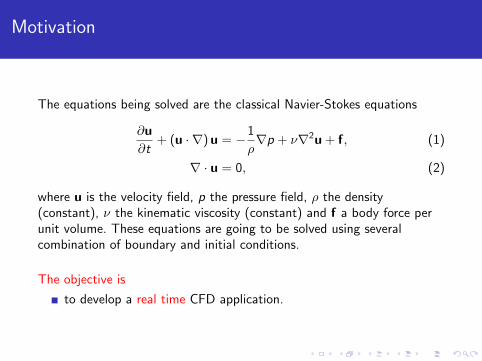
The equations being solved are the classical Navier-Stokes equations

∂u

∂t+ (u · ∇) u = −1

ρ∇p + ν∇2u + f, (1)

∇ · u = 0, (2)

where u is the velocity field, p the pressure field, ρ the density(constant), ν the kinematic viscosity (constant) and f a body force perunit volume. These equations are going to be solved using severalcombination of boundary and initial conditions.

The objective is

to develop a real time CFD application.

QUICK’s workload distribution

Momentum Poisson0

10

20

30

40

50

60

70

80

% c

ompu

ting

time

643

1283

1923

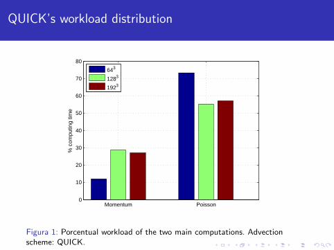
Figura 1: Porcentual workload of the two main computations. Advectionscheme: QUICK.

QUICK’s workload distribution (cont.)

The most important consideration that is involved with Figure 1 is thatthe Poisson step is the most time consuming step in the Fractional-Stepalgorithm used in the solution of Navier-Stokes equations.

In order to speed up the simulations one can choose between manydifferent situations. Thus, one option is

trying to perform the least amount of Poisson steps;

but as QUICK needs to satisfy the CFL (Courant-Friedrichs-Lewycondition) constraint, some other scheme can be proposed in orderto relax this drawback;

so, the Method of Characteristic (MOC) is used as a solution.

Method of characteristics

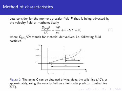
Lets consider for the moment a scalar field F that is being advected bythe velocity field u; mathematically

D(m)F

Dt=∂F

∂t+ u · ∇F = 0, (3)

where D(m)/Dt stands for material derivatives, i.e. following fluidparticles.

x

t

AA'

B

C

Figura 2: The point C can be obtained driving along the solid line (AC), orapproximately, using the velocity field as a first order predictor (dashed lineA′C).

Method of characteristics (cont.)

Analysis of stability properties of the Semi-Lagrangian advection schemeshows that it is possible to stably integrate it for CFL numbers greaterthan unit. In fact, in the simulations performed CFL’s up to 5 are used.

BFECC method

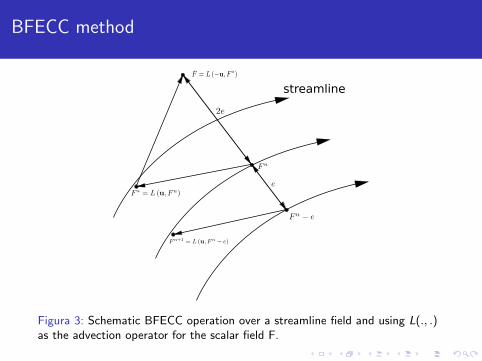
streamline

Figura 3: Schematic BFECC operation over a streamline field and using L(., .)as the advection operator for the scalar field F.

BFECC method (cont.)

Considering the advection operator L(., .) as the Semi-Lagrangian one,BFECC is defined as follows

F ∗ = L (u,F n) (4)

F = L (−u,F ∗) (5)

F ∗ = F n +(F n − F

)/2 (6)

F n+1 = L (u,F ∗) (7)

In this way the order of accuracy of the Semi-Lagrangian scheme can beraised from one to two increasing the amount of work by a factor of three.

CUDA implementation details

The whole Fractinal Step algorithm was implemented in CUDA 1, usingthe tools provided by Thrust 2 and Cusp 3 for linear algebra operations.The FFT used was that provided by CUDA, CUFFT 4.

1https://developer.nvidia.com/what_cuda2http://code.google.com/p/thrust3http://code.google.com/p/cusp_library4https://developer.nvidia.com/cufft

MOC+BFECC’s workload distribution

Momentum Poisson0

10

20

30

40

50

60

70

80

90

% c

ompu

ting

time

643

1283

1923

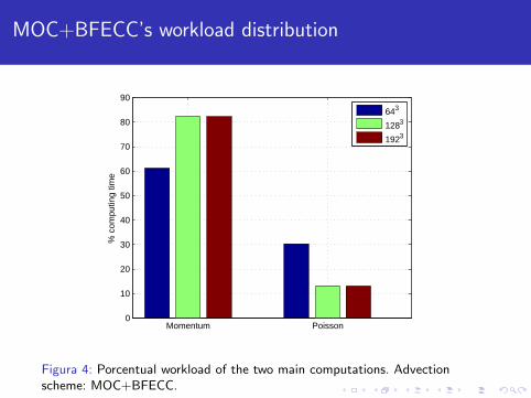
Figura 4: Porcentual workload of the two main computations. Advectionscheme: MOC+BFECC.

2D study case: lid-driven cavity

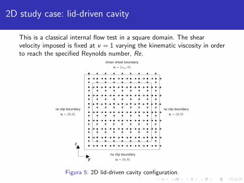
This is a classical internal flow test in a square domain. The shearvelocity imposed is fixed at v = 1 varying the kinematic viscosity in orderto reach the specified Reynolds number, Re.

y

z

no slip boundary no slip boundary

no slip boundary

shear sheet boundary

Figura 5: 2D lid-driven cavity configuration.

2D study case: lid-driven cavity

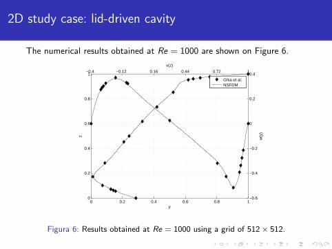
The numerical results obtained at Re = 1000 are shown on Figure 6.

0 0.2 0.4 0.6 0.8 1−0.6

−0.4

−0.2

0

0.2

0.4

y

w(y

)

−0.4 −0.12 0.16 0.44 0.72 1

0

0.2

0.4

0.6

0.8

1

v(z)

z

Ghia et al.NSFDM

Figura 6: Results obtained at Re = 1000 using a grid of 512× 512.

2D study case: lid-driven cavity (cont.)

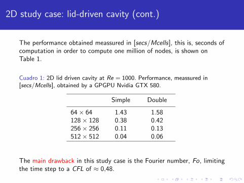
The performance obtained meassured in [secs/Mcells], this is, seconds ofcomputation in order to compute one million of nodes, is shown onTable 1.

Cuadro 1: 2D lid driven cavity at Re = 1000. Performance, meassured in[secs/Mcells], obtained by a GPGPU Nvidia GTX 580.

Simple Double

64× 64 1.43 1.58128× 128 0.38 0.42256× 256 0.11 0.13512× 512 0.04 0.06

The main drawback in this study case is the Fourier number, Fo, limitingthe time step to a CFL of ≈ 0,48.

2D study case: flow past circular cylinder

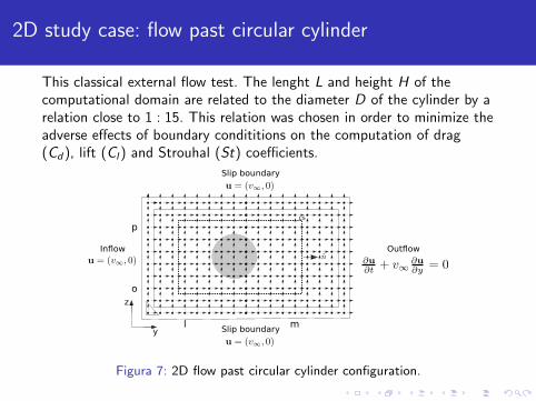
This classical external flow test. The lenght L and height H of thecomputational domain are related to the diameter D of the cylinder by arelation close to 1 : 15. This relation was chosen in order to minimize theadverse effects of boundary condititions on the computation of drag(Cd), lift (Cl) and Strouhal (St) coefficients.

Slip boundary

Inflow Outflow

y

z

CS

Slip boundaryl m

o

p

Figura 7: 2D flow past circular cylinder configuration.

2D study case: flow past circular cylinder (cont.)

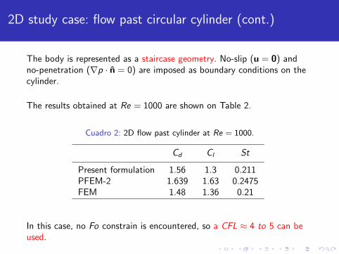
The body is represented as a staircase geometry. No-slip (u = 0) andno-penetration (∇p · n = 0) are imposed as boundary conditions on thecylinder.

The results obtained at Re = 1000 are shown on Table 2.

Cuadro 2: 2D flow past cylinder at Re = 1000.

Cd Cl St

Present formulation 1.56 1.3 0.211PFEM-2 1.639 1.63 0.2475FEM 1.48 1.36 0.21

In this case, no Fo constrain is encountered, so a CFL ≈ 4 to 5 can beused.

2D study case: flow past circular cylinder (cont.)

0 50 100 150 200 250 300 350 400 450−1.5

−1

−0.5

0

0.5

1

1.5

2Re = 1000

t∗ = v∞t(1/2)D

CLCD

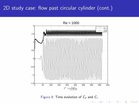
Figura 8: Time evolution of Cd and Cl .

3D study case: lid-driven cavity

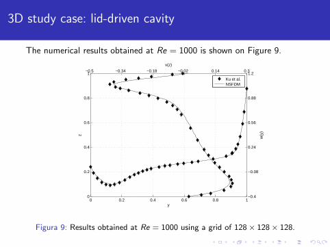
The numerical results obtained at Re = 1000 is shown on Figure 9.

0 0.2 0.4 0.6 0.8 1−0.4

−0.08

0.24

0.56

0.88

1.2

y

w(y

)

−0.5 −0.34 −0.18 −0.02 0.14 0.3

0

0.2

0.4

0.6

0.8

1

v(z)

z

Ku et al.NSFDM

Figura 9: Results obtained at Re = 1000 using a grid of 128× 128× 128.

3D study case: lid-driven cavity (cont.)

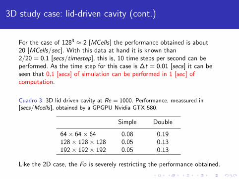
For the case of 1283 ≈ 2 [MCells] the performance obtained is about20 [MCells/sec]. With this data at hand it is known than2/20 = 0,1 [secs/timestep], this is, 10 time steps per second can beperformed. As the time step for this case is ∆t = 0,01 [secs] it can beseen that 0,1 [secs] of simulation can be performed in 1 [sec] ofcomputation.

Cuadro 3: 3D lid driven cavity at Re = 1000. Performance, meassured in[secs/Mcells], obtained by a GPGPU Nvidia GTX 580.

Simple Double

64× 64× 64 0.08 0.19128× 128× 128 0.05 0.13192× 192× 192 0.05 0.13

Like the 2D case, the Fo is severely restricting the performance obtained.

3D study case: lid-driven cavity (cont.)

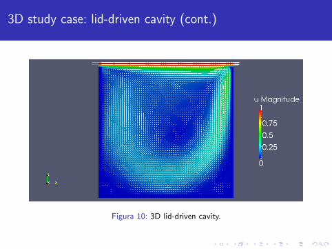
Figura 10: 3D lid-driven cavity.

3D study case: flow past circular cylinder

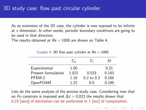
As an extension of the 2D case, the cylinder is now suposed to be infiniteat x dimension. In other words, periodic boundary conditions are going tobe used in that direction.The results obtained at Re = 1000 are shown on Table 4.

Cuadro 4: 3D flow past cylinder at Re = 1000.

Cd Cl St

Experimental 1.00 0.21Present formulation 1.021 0.533 0.183PFEM-2 1.16 0.2 to 0.3 0.185OpenFOAM 1.22 0.5 0.195

Lets do the same analysis of the previos study case. Considering now thatno Fo constrain is imposed and ∆t = 0,023 the results shown that0,23 [secs] of simulation can be performed in 1 [sec] of computation.

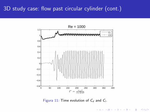
3D study case: flow past circular cylinder (cont.)

0 50 100 150 200 250 300 350 400−0.8

−0.6

−0.4

−0.2

0

0.2

0.4

0.6

0.8

1

1.2Re = 1000

t∗ = v∞t(1/2)D

CLCD

Figura 11: Time evolution of Cd and Cl .

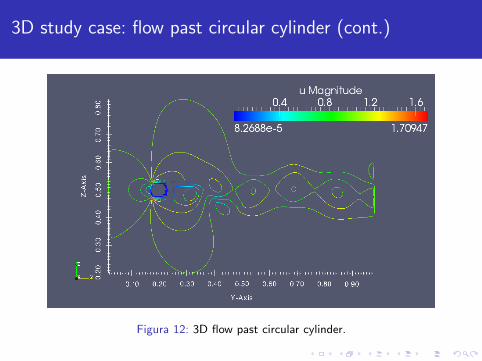
3D study case: flow past circular cylinder (cont.)

Figura 12: 3D flow past circular cylinder.

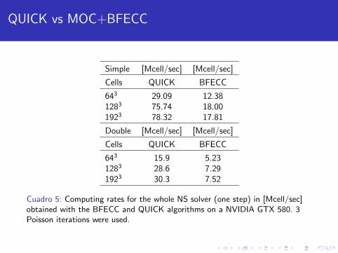
QUICK vs MOC+BFECC

Simple [Mcell/sec] [Mcell/sec]

Cells QUICK BFECC

643 29.09 12.381283 75.74 18.001923 78.32 17.81

Double [Mcell/sec] [Mcell/sec]

Cells QUICK BFECC

643 15.9 5.231283 28.6 7.291923 30.3 7.52

Cuadro 5: Computing rates for the whole NS solver (one step) in [Mcell/sec]obtained with the BFECC and QUICK algorithms on a NVIDIA GTX 580. 3Poisson iterations were used.

QUICK vs MOC+BFECC (cont.)

As a reference, the QUICK algorithm was implemented in CPU obtaininga rate of 3.5 [Mcell/sec] (OpenMP) on an Intel i7-3820@3.47 GHz (SandyBridge microarchitecture) for large 3D meshes (above 1 Mcell), i.e. 8.6times slower with respect to the GPU(QUICK) version. Note that thisspeedup obtained on the GPU is close to the 8x speedup factor obtainedfor the FFT. This is normal, because for the QUICK implementation alarge part of the computing time is spent in the Poisson step.

The BFECC(GPU) is only 2.15 times faster than the QUICK(CPU)version in Mcells/sec, but taking into account that the CFL is 10 timeslarger, the overall speedup is 21.5, i.e. BFECC(GPU) is 21.5 times fasterthan QUICK(CPU) in computing one second of the same physicalprocess.

Conclusions

A CUDA implementation of the 3D viscous Navier-Stokes equationswas presented and its accuracy and performance were obtained usingtwo well-known study cases.

The results shown good agreement with the references and, whenCFL > 2, BFECC performs better than the previous advectionscheme, QUICK.

It must be recalled that, bodies are stair-case defined andrefinements are being explored by the authors at the moment.

Also, new ways of solving diffusion equations is being studied too.

Acknowledge

This work has received financial support of

Agencia Nacional de Promocion Cientıfica y Tecnologica (ANPCyT,Argentina, grants PICT-1141/2007, PICT-0270/2008),

Universidad Nacional del Litoral (UNL, Argentina, grants CAI+D2009-65/334, CAI+D-2009-III-4-2) y

European Research Council (ERC) Advanced Grant, Real TimeComputational Mechanics Techniques for Multi-Fluid Problems(REALTIME, Reference: ERC-2009-AdG, Dir: Dr. Sergio Idelsohn).

Also we use some development tools under Free Software likeGNU/Linux OS, GCC/G++ compilers, Octave, and Open Sourcesoftware like VTK, among many others.