The Einstein-Vlasov system in spherical symmetry II: spherical perturbations of staticsolutions

Carsten Gundlach(Dated: 24 August 2017)

We reduce the equations governing the spherically symmetric perturbations of static sphericallysymmetric solutions of the Einstein-Vlasov system (with either massive or massless particles) to asingle stratified wave equation −ψ,tt = Hψ, with H containing second derivatives in radius, andintegrals over energy and angular momentum. We identify an inner product with respect to whichH is symmetric, and use the Ritz method to approximate the lowest eigenvalues of H numerically.For two representative background solutions with massless particles we find a single unstable modewith a growth rate consistent with the universal one found by Akbarian and Choptuik in nonlinearnumerical time evolutions.

CONTENTS

I. Introduction 1A. The Einstein-Vlasov system 1B. Motivation for this paper 1C. Plan of the paper 2

II. Background equations 2A. Field equations in spherical symmetry 2B. Static solutions 3C. Reduction of the field equations for m = 0 4

III. Spherical perturbation equations 4A. Perturbation ansatz 4B. Change of variable from z to Q 5C. Static perturbations 5D. Reduction to a single stratified wave

equation 5E. Preliminary classification of non-static

perturbations 6F. Massless case 7

IV. Perturbation spectrum 7A. Inner product 7B. Quadratic form of the Hamiltonian 8C. Ritz method 9D. The space of test functions ψ 9E. Numerical examples of the Ritz method for

massless particles 10

V. Conclusions 12

Acknowledgments 12

References 13

I. INTRODUCTION

A. The Einstein-Vlasov system

The Vlasov-Einstein system describes an ensemble ofparticles of identical rest mass, each of which follows ageodesic. The particles interact with each other only

through the spacetime curvature generated by their col-lective stress-energy tensor, whereas particle collisionsare neglected.

For massive particles, this is a good physical modelof a stellar cluster. For either massive or massless par-ticles, the Einstein-Vlasov system also serves as a well-behaved toy model of matter in general relativity. In par-ticular, spherically symmetric solutions of the Einstein-Vlasov system with small data are known to exist glob-ally in time for massive [1] and massless particles [2].Self-similar spherically symmetric solutions with mass-less particles have been analyzed in [3] and [4]. Theexistence of spherically symmetric static solutions withmassive particles was proved in [5], and there is numeri-cal evidence that at least some are stable within spheri-cal symmetry [6]. Spherically symmetric static solutionswith massless particles were analysed and constructednumerically in [7], and we investigate their linear per-turbations here. See also [8] for a review and additionalreferences.

B. Motivation for this paper

This is the second paper in a series motivated byAkbarian and Choptuik’s [9] (from now on, AC) re-cent study of numerical time evolutions of the masslessEinstein-Vlasov system in spherical symmetry. AC foundtwo apparently contradictory results:

I) Taking several 1-parameter families of genericsmooth initial data and fine-tuning the parameter tothe threshold of black hole formation, AC found what isknown as type-I critical collapse: in the fine-tuning limitthe time evolution goes through an intermediate staticsolution. The lifetime ∆τ of this static solution increaseswith fine-tuning to the collapse threshold as

∆τ ' σ ln |p− p∗|+ const, (1)

where p is the parameter of the family, p∗ its value atthe black-hole threshold, and τ is the proper time atthe centre, in units of the total mass of the critical so-lution. (1) implies the existence of a single unstablemode growing as exp(τ/σ). AC found that σ was ap-proximately universal (independent of the family), with

arX

iv:1

708.

0719

1v1

[gr

-qc]

23

Aug

201

7

2

value σ ' 1.4 ± 0.1, and that the metric of the inter-mediate static solution was also approximately universal(up to an overall length and mass scale). In particu-lar, its compactness Γ := max(2M/r) was in the rangeΓ ' 0.80±0.01 and its central redshift Zc ≥ 0 was in therange Zc ' 2.45± 0.05.

II) Conversely, constructing static solutions by ansatz,AC found that these covered much larger ranges of Γand Zc, but that each one was at the threshold of col-lapse. That is, adding a small generic perturbation to thestatic initial data and evolving in time with their nonlin-ear code, they found that for one sign of the perturbationthe perturbed static solution collapsed while for the othersign it dispersed. They found that σ was in the narrowrange σ ' 1.43± 0.07, compatible with the value above.

Result II suggests that in spherical symmetry withmassless particles, the black hole-threshold coincideswith the space of static solutions. If so, then each staticsolution would have precisely one unstable mode (withits sign deciding between collapse and dispersion), withall other modes either zero modes (moving to a neigh-bouring static solution) or purely oscillating.

One aspect of Result I, namely that the spacetime ofthe critical solution is universal, would imply that thisuniversal solution has one unstable mode (as before), butthat all its other modes (including those tangential to theblack hole threshold) are decaying ones, so that the at-tracting manifold of the critical solution is precisely theblack hole threshold. Indeed, this is the familiar pic-ture of type-I critical collapse in other matter-Einsteinsystems. However, this is in apparent contradiction toResult II.

In the first paper in this series [7] (from now PaperI), we used a symmetry of the massless spherically sym-metric Einstein-Vlasov system to reduce its number ofindependent variables from four to three. We then nu-merically constructed static solutions with compactnessin the range 0.7 ' Γ ≤ 8/9. Based on this, we conjec-tured that the apparent contradiction above is resolvedby the critical solution seen in fine-tuning generic initialdata being universal only to leading order, and that thisleading order is selected by the way in which it is ap-proached during the evolution of generic smooth initialdata.

To make further progress, it seems essential to analysethe spectrum of linear perturbations directly. This is theprogramme of the current paper. In contrast to the staticsolutions investigated in Paper I, their perturbations donot simplify significantly for m = 0, and hence all of ouranalysis, except for the numerical examples in Sec. IV E,will be for m ≥ 0.

C. Plan of the paper

In order to make the presentation self-contained andto establish notation, we review some material from Pa-per I in Sec. II. We begin in Sec. II A by presenting the

equations of the time-dependent spherically symmetricEinstein-Vlasov system. We do this in a form in whichthe massless particle limit is regular and leads to a reduc-tion of the number of independent variables. We discussstatic solutions in Sec. II B, and the massless limit, forboth the time-dependent and static case, in Sec. II C.

In Sec. III we then derive the spherical perturbationequations. In Sec. III A we perturb the Vlasov and Ein-stein equations about a static background, splitting theperturbation of the Vlasov distribution function f intoparts φ and ψ that are even and odd, respectively un-der reversing time. In Sec. III B we change independentvariables from momentum to energy, as we did for thebackground solutions. We quickly dispense with staticperturbations in Sec. III C, and in Sec. III D we reducethe perturbed Vlasov and Einstein equations to a singleintegral-differential equation −ψ,tt = Hψ. In Sec. III Ewe dispense with the relatively trivial perturbations onregions of phase space where the background solution isvacuum. We state the massless limit in Sec. III F.

In Sec. IV we attempt to find the spectrum of eigen-values. In Sec. IV A we identify a positive definite in-ner product with respect to which H is symmetric. InSec. IV B we rewrite the Hamiltonian as H = A†A−D†Dwhere D is bounded, giving us at least a lower bound onH. We then switch to an approximation method, theRitz method, which we review in Sec. IV C. In Sec. IV Dwe specify some properties of the function space V inwhich to look for perturbation modes, that is eigenfunc-tions of H. In Sec. IV E we pick two specific backgroundsolutions that we obtained numerically in Paper I anduse the Ritz method numerically. We find values of σ inagreement with AC.

Sec. V contains a summary and outlook. Throughoutthe paper, a := b defines a, and we use units such thatc = G = 1.

II. BACKGROUND EQUATIONS

A. Field equations in spherical symmetry

We consider the Einstein-Vlasov system in sphericalsymmetry, with particles of mass m ≥ 0. We write themetric as

ds2 = −α2(t, r)dt2+a2(t, r)dr2+r2(dθ2+sin2 θdϕ2). (2)

To fix the remaining gauge freedom we set α(t,∞) = 1.The Einstein equations give the following equations forthe first derivatives of the metric coefficients:

α,rα

=a2 − 1

2r+ 4πra2p, (3)

a,ra

= −a2 − 1

2r+ 4πra2ρ, (4)

a,ta

= 4πra2j, (5)

3

where p, ρ and j are the radial pressure, energy densityand radial momentum density, measured by observers atconstant r. The fourth Einstein equation, involving thetangential pressure pT , is a combination of derivativesof these three, and is redundant modulo stress-energyconservation.

The Vlasov density describing collisionless matter ingeneral relativity is defined on the mass shell pµpµ =−m2 of the cotangent bundle of spacetime, or f(t, xi, pi)in coordinates. We define the square of particle angularmomentum

F := p2θ + sin2 θ p2ϕ. (6)

In spherical symmetry this is conserved, leaving to f =f(t, r, pr, F ). In order to obtain a reduction of theEinstein-Vlasov system in the limit m = 0, we replacepr by the new independent variable

z :=pr

a√F. (7)

The Vlasov equation for f(t, r, z, F ) is

∂f

∂t+αz

aZ

∂f

∂r+

(α

r3aZ− α,rZ

a− za,t

a

)∂f

∂z= 0, (8)

where we have defined the shorthand

Z(r, z, F ) :=

√m2

F+ z2 +

1

r2=αpt√F. (9)

The non-vanishing components of the stress-energytensor are

p := Trr =

π

r2J f z

2

Z, (10)

ρ := −Ttt =π

r2J f Z, (11)

j := Ttr = − π

r2α

aJ f z, (12)

pT := Tθθ = Tϕ

ϕ =π

2r4J f 1

Z, (13)

where we have introduced the integral operator (actingto the right)

J :=

∫ ∞0

FdF

∫ ∞−∞

dz. (14)

B. Static solutions

In the static metric

ds2 = −α20(r)dt2 + a20(r)dr2 + r2(dθ2 + sin2 θdϕ2) (15)

with Killing vector ξ := ∂t, the particle energy

E := −ξµpµ = −pt = α0

√FZ (16)

is conserved along particle trajectories. In order to obtaina reduction of the static Einstein-Vlasov system in thelimit m = 0, we replace E by

Q(r, z, F ) :=E2

F= α2

0Z2. (17)

Hence we have

z = ±α0(r)√Q− U, (18)

where we have defined

U(r, F ) := α20

(m2

F+

1

r2

). (19)

The general static solution of the Vlasov equation, forsimplicity with a single potential well, is then given by

f(r, z, F ) = k(Q,F ). (20)

(If U forms more than one potential well, k could bedifferent in each of them [10].)

The static Einstein equations are

α′0α0

=a20 − 1

2r+

4π2a20rIkv, (21)

a′0a0

= −a20 − 1

2r− 4π2a20

rI kv, (22)

where we have defined the integral operator (acting tothe right)

I :=

∫ ∞0

FdF

∫ ∞U(r,F )

dQ (23)

and the shorthand

v(r,Q, F ) :=|z|Z

=a|pr|αpt

. (24)

From (17) and (9) we have dQ = 2α20z dz, and hence on

a static background, where I is defined, it is related toJ by

I = α20J z. (25)

The second equality in (24) shows that ±v is the ra-dial particle velocity, expressed in units of the speed oflight and measured by static observers. (Note that bydefinition v ≥ 0.) The fact that (24) can be rewritten as

v =

√1− U

Q(26)

shows that U is an effective potential for the radialmotion of the particles with given constant “energy”Q and angular momentum squared F . In particularQ = U(r, F ) determines the radial turning points r forall particles with a given Q and F .

4

We define U0(F ) as the value of U(r, F ) at its onelocal maximum r0+(F ) in r. We define r0−(F ) as theother value of r for which U takes the same value. Wealso define U3(F ) as the value of U(r, F ) at its one localminimum r3(F ) in r. Intuitively, U0(F ) is the “lip” of theeffective potential for particles of a given F , and U3(F )its “bottom”. We define U1(F ) ≤ U0(F ) as the upperboundary in Q of the support of k(Q,F ) and U2(F ) ≥U3(F ) as the lower boundary. We define r1±(F ) andr2±(F ) as the values where Q = U1(F ) or Q = U2(F ).

For massless particles, particles with all values of Fmove in the same potential U = U(r), and all otherquantities we have just defined do also not depend onF . See Fig. 1 for an illustration.

Any particles with Q > U0(F ) would be unbound, andif such particles were present in a static solution with theansatz (20) they would be present everywhere and hencethe total mass could not be finite. We must thereforehave k(Q,F ) = 0 for Q > U0(F ). k(Q,F ) must eitherhave compact support in F , or fall off as F → ∞ suffi-ciently rapidly for

∫kFdF to be finite. Both assumptions

are assumed implicitly in the definition (23) of I whenwe formally extend the upper integration limits in Q andF to ∞.

By contrast, real values of z require Q ≥ U(r, F ), andwhen changing from

∫dz to

∫dQ, the condition Q ≥ U

must be imposed explicitly as a limit to the integrationrange in (23). Hence k(Q,F ) needs to be defined for allU3(F ) ≤ Q ≤ U0(F ) (it can be zero in part of that range),but not all of that range contributes to the integral I, andhence to the stress-energy tensor, at every value of r.

C. Reduction of the field equations for m = 0

Because F is conserved, the field equations already donot contain ∂/∂F . Furthermore, m and F appear in thecoefficients of the field equations only in the combinationm2/F . In the limit m = 0, these coefficients becomeindependent of F . As first used in [3], the integratedVlasov density

f(t, r, z) :=

∫ ∞0

f(t, r, z, F )FdF (27)

then obeys the same PDE (8) as f itself. The stress-energy tensor is now given by the expressions (10-13)above, with f in place of f , and

J :=

∫ ∞−∞

dz (28)

in place of J . We have reduced the Einstein-Vlasov sys-tem to a system of integral-differential equations in theindependent variables (t, r, z) only. A solution (a, α, f)of the reduced system represents a class of solutions(a, α, f), all with the same spacetime but different matterdistributions.

Similarly, in the static case with m = 0 the Einsteinequations are given by (21-22) with

k(Q) :=

∫ ∞0

k(Q,F )FdF (29)

in place of k(Q,F ) and

I :=

∫ ∞U(r)

dQ (30)

in place of I. Each solution of the reduced system(a0, α0, k) represents a class of solutions (a0, α0, k). Wenow define U1 and U2 as the limits of support of k(Q).

In Paper I, we conjectured that the space of spheri-cally symmetric static solutions with massless particlesis a space of single functions of one variable, subject tocertain positivity and integrability conditions. This sin-gle function can be taken to be any one of α0(r), a0(r)or k(Q).

As a postscript to Paper I, we note here that a mathe-matically similar result holds for Vlasov-Poisson systemfor a subclass of static solutions, namely the “isotropic”ones, where the Vlasov function is assumed to be a func-tion of energy only. With the isotropic ansatz the Vlasovdensity uniquely defines the Newtonian gravitational po-tential and vice versa [11]. Physically, however, the tworesults are different, as the relativistic result with mass-less particles holds for all solutions, depending on bothenergy and angular momentum.

III. SPHERICAL PERTURBATIONEQUATIONS

A. Perturbation ansatz

In the study of the linear perturbations of a static so-lution we return to the general case m ≥ 0. We make theperturbation ansatz

α(t, r) = α0(r) + δα(t, r), (31)

a(t, r) = a0(r) + δa(t, r), (32)

f(t, r, z, F ) = k(Q,F ) + φ(t, r, z, F )

+ψ(t, r, z, F ), (33)

where (α0, a0, k) is a static solution of the Einstein-Vlasov system, and where Q is given by (17). We de-fine φ to be even in z and ψ to be odd. In particular,as δf(t, r, z, F ) must be at least once continuously differ-entiable (C1) to obey the Vlasov equation in the strongsense, its odd-in-z part must vanish at z = 0, or

ψ(t, r, z = 0, F ) = 0. (34)

We now expand to linear order in the perturbations.The linearised Vlasov equation splits into the pair

φ,t + Lψ = 2Qk,Qv2

a0δa,t, (35)

ψ,t + Lφ = 2Qk,Qvα0

a0

(δα

α0

),r

, (36)

5

where we have defined the differential operator

L :=zα0

Za0

∂

∂r+

(α0

a0r3Z− Zα′0

a0

)∂

∂z. (37)

Note, from (8), that the time-dependent Vlasov equationin the fixed static spacetime (a0, α0) is f,t + Lf = 0. Byconstruction, Q obeys LQ = 0, and hence Lk(Q,F ) = 0,as we have already used to construct static solutions. Theeven-odd split of the perturbed Vlasov equation into thepair (35,36) reflects the fact that reversing both t and ztogether must leave the field equations invariant.

The perturbed Einstein equations are(δα

α0

),r

−(

1

r+

2α′0α0

)δa

a0=

4π2a20rJ z

2

Zφ, (38)(

rδa

a30

),r

= 4π2JZφ, (39)

δa,t = −4π2a20rJ zψ. (40)

We have used the background Einstein equations to elim-inate all integrals of k in favour of a′0 and α′0. Theintegrability condition for δa between (39) and (40) isidentically obyed modulo the perturbed Vlasov equation(35,36), and hence the perturbed Einstein equation (40)is redundant [just as (5) is in the nonlinear equations].

B. Change of variable from z to Q

To simplify the perturbation equations, we change in-dependent variables from (t, r, z, F ) to (t, r,Q, F ), with Qagain given by (17). From the resulting transformation ofpartial derivatives, we need only the following identities:

∂

∂t

∣∣∣∣z

=∂

∂t

∣∣∣∣Q

, (41)

∂

∂r

∣∣∣∣z

=∂

∂r

∣∣∣∣Q

+ (. . . )∂

∂Q

∣∣∣∣r

, (42)

L = V∂

∂r

∣∣∣∣Q

, (43)

where we have defined the shorthand

V (r,Q, F ) =α0

a0v, (44)

with v given by (26). V is the coordinate speed dr/dtcorresponding to the physical speed v.∂/∂r|z on its own appears in the field equations only

acting on the metric and its perturbations, in which casethe ∂/∂Q|r term denoted by (. . . ) in (42) is irrelevant.On the matter perturbations, ∂/∂r|z acts only in thecombination L. From now on ∂/∂r is understood to mean∂/∂r|Q.

With (43) the perturbed Vlasov equation becomes

φ,t + V ψ,r = 2Qk,Qv2

a0δa,t, (45)

ψ,t + V φ,r = 2Qk,Qvα0

a0

(δα

α0

),r

. (46)

With (25) and (24) the perturbed Einstein equations(38-40) become(

δα

α0

),r

−(

1

r+

2α′0α0

)δa

a0=

4π2a20rα2

0

Ivφ, (47)(rδa

a30

),r

=4π2

α20

I φv, (48)

δa,t = −4π2a20rα0

Iψ. (49)

Equivalently, the stress-energy perturbations are givenby

δp =π

r2α20

Ivφ, (50)

δρ =π

r2α20

I φv, (51)

δj = − π

r2α0a0Iψ. (52)

Finally, the boundary condition on ψ becomes

ψ(t, r, U(r, F ), F ) = 0. (53)

C. Static perturbations

Static perturbations can be obtained more directly bylinear perturbation of the nonlinear static equations. Theinfinitesimal change k → k + δk, a0 → a0 + δa0, α0 →α0 + δα0 to a neighbouring static solution gives

φ =d

dε

∣∣∣∣ε=0

(k + εδk)((α0 + εδα)2Z2, F

)= δk(Q,F ) + 2Qk,Q

δα

α0, (54)

ψ = 0. (55)

As expected, this solves the perturbed Vlasov equations(45-46) and Einstein equation (49) identically for ar-bitrary functions δk(Q,F ), modulo the nontrivial per-turbed Einstein equations (47-48).

D. Reduction to a single stratified wave equation

We can uniquely split any time-dependent perturba-tion that admits a Fourier transform with respect to tinto a static part (with frequency ω = 0) and a genuinelynon-static part (with frequencies ω 6= 0). For genuinelynon-static perturbations we can uniquely invert ∂/∂t bydividing by iω in the Fourier domain.

6

We now substitute (49) into (45), and (47) and(∂∂t

)−1(49) into (46), and write the result in the com-

pact form ( ∂∂t A

B ∂∂t +

(∂∂t

)−1C

)(φψ

)= 0, (56)

where we have defined the integral-differential operators(acting to the right)

A := L+ gvI, (57)

B := L− gIv, (58)

C := hgI (59)

with the differential operator L now given by (43), theintegral operator I defined in (23) (both acting to theright), v given by (26), and the shorthand expressions

g(r,Q, F ) :=8π2a0rα0

Qk,Q v, (60)

h(r) :=α0

a0

(1

r+

2α′0α0

). (61)

Note that A, B, C do not commute with each other, while∂/∂t commutes with all of them because their coefficientsare independent of t.

In this compact notation it is easy to see that by rowoperations we can reduce the system (56) to the upperdiagonal form( ∂

∂t A

0(∂∂t

)2+ C −BA

)(φψ

)= 0. (62)

Hence we have reduced the time-dependent problem tothe single integral-differential equation

− ψ,tt = Hψ, (63)

where

H := C −BA = hgI − (L− gIv)(L+ gvI). (64)

The coefficients g, h, v and V commute with each otherbut not with the operators ∂/∂r or I. ∂/∂r and I docommute with each other because of the boundary con-dition (53).

It is convenient to split the time evolution operator Hinto a kinematic and a gravitational part as

H = H0 +H1, (65)

with

H0 := −L2 = −V ∂

∂rV∂

∂r, (66)

H1 := g(h+

(Iv2g

))I + gIvL− LgvI (67)

=[g(h+

(Iv2g

))− (Lgv)

]I + g (IvL− vLI) .

(68)

Hence we can write (63) as

− ψ,tt + V∂

∂rV∂

∂rψ = H1ψ. (69)

This form stresses that (69) is a stratified wave equa-tion, in the sense that for fixed Q and F we have a waveequation in (t, r), with coefficients also depending on Qand F , while different values of Q and F are also cou-pled through the double integral I over Q and F , whichrepresents the gravitational interactions between parti-cles of different momenta at the same spacetime point.Intuitively, the characteristic speeds of (69) are ±V be-cause any matter perturbation is propagated simply atthe velocity of its constituent particles.

We note in passing that in our notation the static per-turbations are solutions of

Bφ = 0, ψ = 0. (70)

Given a solution ψ of the master equation (63), φ in anygenuinely nonstatic perturbation can be reconstructedfrom ψ as

φ = −(∂

∂t

)−1Aψ, (71)

and the metric perturbations are obtained by solving (47-48), with (49) obeyed automatically.

E. Preliminary classification of non-staticperturbations

The right-hand side of (69) is generated by pertur-bations at all values of Q and F at at given space-time point (t, r), but because of the overall factor k,Qit only acts on perturbations at those values of Q and Fwhere k,Q(Q,F ) 6= 0, that is, where background matteris present.

This suggests a preliminary classification of all pertur-bations into

• stellar modes, with support on the region in(r,Q, F ) space that lies inside the potential welland where also k(Q,F ) has support;

• bottom modes, with support inside the potentialwell and for values of Q below the support ofk(Q,F );

• middle modes, with support inside the potentialwell and for values of Q above the support ofk(Q,F ) but below the top of the potential well;

• outer modes, with support outside the potentialwell and for values of Q below the top of the po-tential well;

• top modes, with values of Q above the top of thepotential well.

7

r0 - r0 +r1 - r1 +r2 - r2 +r3

U0

U1

U2

U3

r

U

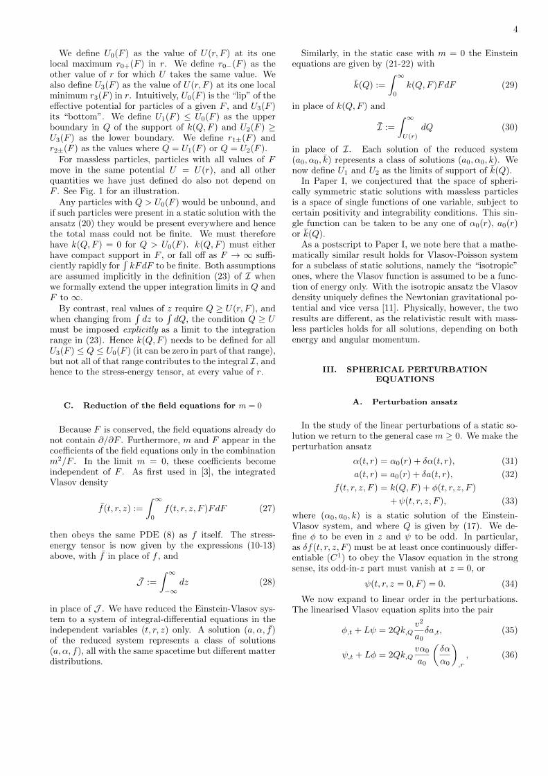
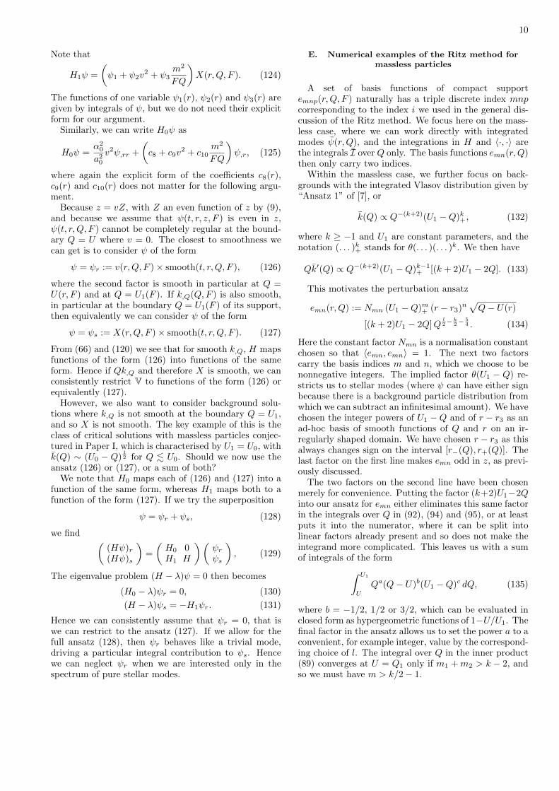
FIG. 1. Sketch of the potential U(r) for massless parti-cles, illustrating the classification of perturbations. The blackhatching shows the region in (U, r) space where particles arepresent in the background solution. Outer modes have sup-port in the green region, top modes in the yellow region, mid-dle modes in the red region, bottom modes in the blue region,and stellar modes in the hatched region only. (The top, mid-dle and bottom modes also drive stellar modes.) This figurecan also be interpreted as the cross-section U(r,∞) of thepotential U(r, F ) in the massive case, compare the definition(19) of U .

This classification of modes is illustrated in Fig. 1 for themassless case, where all values of F experience the sameeffective potential U(r). Obviously, the middle modes donot exist if the potential well is filled to the top (U1 =U0), and the bottom modes do not exist if it is filled tothe bottom (U2 = U3).

Particles contributing to the bottom, middle, top andouter modes move freely in the effective potential U(r, F )set by the static background solution, without experienc-ing a gravitational back-reaction. We may call them thetrivial modes. Mathematically, the trivial modes obey(69) in a region of (Q,F ) space where the right-handside vanishes. In that region they can be solved in closedform. To do this, we define the “tortoise radius”

σ(r,Q, F ) :=

∫ r 1

V (r′, Q, F )dr′. (72)

This gives us

L = V∂

∂r

∣∣∣∣Q

=∂

∂σ

∣∣∣∣Q

, (73)

and hence (69) becomes

− ψ,tt + ψ,σσ = 0 (74)

for ψ(t, σ,Q, F ), subject to the Dirichlet boundary con-ditions

ψ(t, σ−(Q,F ), Q, F ) = ψ(t, σ+(Q,F ), Q, F ) = 0, (75)

where σ± are the left and right turning points given byQ = U . Hence we can write down the general local solu-

tion of (69) with S = 0 in d’Alembert form as

ψ(t, r,Q, F ) =∑±ψ± [t± σ(r,Q, F ), Q, F ] (76)

subject to the boundary conditions (75).With g = 0 for the trivial modes, (71) becomes φ,t +

ψ,σ = 0, and hence

φ(t, r,Q, F ) =∑±∓ψ± [t± σ(r,Q, F ), Q, F ] . (77)

We note also that ψ+ φ must be non-negative for physi-cal trivial modes, as we cannot subtract particles from avacuum region.

The trivial modes (except for the outer modes) in-duce stellar modes through gravitational interactions, ormathematically through the right-hand side of (69). Thismeans that for a complete solution of the problem, weneed to solve for stellar modes including an arbitrarydriving term generated by the other modes, that is

− ψ,tt + V∂

∂rV∂

∂rψ = H1ψ +H1ψext (78)

where ψ describes the stellar modes and ψext is the sumof the top, middle and bottom modes. (The outer modesdo not couple to the stellar modes at all.)

F. Massless case

In the massless case, we define the integrated matterperturbations in the obvious way:

φ(t, r,Q) :=

∫ ∞0

φ(t, r,Q, F )FdF, (79)

ψ(t, r,Q) :=

∫ ∞0

ψ(t, r,Q, F )FdF. (80)

The reduced perturbation equations with m = 0 are ob-tained from the ones in the general case by replacing φand ψ with φ and ψ, k(Q,F ) and k,Q(Q,F ) with k(Q)and k′(Q), and I with I. The coefficients g, v, V and Uall become independent of F . In particular, all particlesnow move in the same effective potential U(r).

IV. PERTURBATION SPECTRUM

A. Inner product

Starting from (67), we rewrite the gravitational partH1 of the Hamiltonian more explicitly as

H1 = Xc1I +X

(c2Iv2

∂

∂r− ∂

∂rc2v

2I). (81)

8

where we have defined the shorthands

X(Q,F, r) := Qk,QV, (82)

c0(r) :=8π2a20rα2

0

, (83)

c1(r) :=8π2a0rα0

(1

r+

2α′0α0

+ c3

), (84)

c2(r) :=8π2a0rα0

, (85)

c3(r) :=8π2a20rα2

0

Iv3Qk,Q. (86)

We have defined c0 for later use: note that g = c0X.For clarity we have not written out function arguments,but recall that I acting on anything gives a function oft and r only, that k = k(Q,F ), v2 = 1 − U/Q, U =U(r,m2/F ), and hence that v = v(r,Q,m2/F ) and V =V (r,Q,m2/F ).

We now construct an inner product 〈ψ1, ψ2〉 with re-spect to which H is a symmetric operator. Consider firstsolutions ψ1, ψ2 with support only where k,Q(Q,F ) = 0,that is the modes we have characterised as trivial. Thenonly H0ψ is non-vanishing, and the perturbed Vlasovequation reduces to the free wave equation (74). The ob-vious inner product is therefore the well-known one forthe free wave equation, that is

〈ψ1, ψ2〉 :=

∫ ∞0

∫ ∞0

(∫ σ+(Q,F )

σ−(Q,F )

ψ1ψ2 dσ

)µ(Q,F ) dQFdF,

(87)where µ(Q,F ) > 0 is an arbitray weight. Expressing thisin terms of r, we have

〈ψ1, ψ2〉 =

∫ ∞0

∫ ∞0

(∫ r+(Q,F )

r−(Q,F )

ψ1ψ2 dr

V (r,Q, F )

)µ(Q,F ) dQFdF.

(88)If we interchange the integration over r with the double

integration over Q and F , we obtain

〈ψ1, ψ2〉 =

∫ ∞0

∫ ∞0

(∫ ∞U(r,F )

µ(Q,F )ψ1ψ2 dQ

V (r,Q, F )

)FdF dr

=

∫ ∞0

(I µψ1ψ2

V

)dr (89)

Integration by parts in r in (88), and then transformingto (89), then gives

〈ψ1, H0ψ2〉 =

∫ ∞0

(IµV ψ1,rψ2,r) dr = 〈V ψ1,r, V ψ2,r〉,

(90)which is explicitly symmetric in ψ1 and ψ2.

Consider now solutions ψ1, ψ2 with support only wherek,Q(Q,F ) 6= 0, that is stellar modes. Assuming furtherthat k,Q < 0 wherever k 6= 0 (as will be the case for ourexamples), we must then make the choice

µ(Q,F ) = − 1

Qk,Q(91)

(up to a positive constant factor), that is

〈ψ1, ψ2〉 = −∫ ∞0

(Iψ1ψ2

X

)dr (92)

= −∫ ∞0

∫ ∞0

(∫ r+

r−

ψ1ψ2

Xdr

)dQFdF, (93)

with X defined in (82). We then find from (90), (92) and(81) that

〈ψ1, H0ψ2〉 = −∫ ∞0

(I V

2ψ1,rψ2,r

X

)dr, (94)

〈ψ1, H1ψ2〉 = −∫ ∞0

c1(Iψ1)(Iψ2) dr

−∫ ∞0

c2[(Iψ1)(Iv2ψ2,r)

+(Iψ2)(Iv2ψ1,r)]dr, (95)

where for the last term we have used integration by partsin r.

We now define µ(Q,F ) > 0 on all of phase space by(91) on the support of k(Q,F ), and an arbitrary positiveµ, for example µ = 1, everywhere else.

B. Quadratic form of the Hamiltonian

Consider the operator

P :=XI

(IX). (96)

It is easy to see that P is a projection operator, in thesense that

P 2 = P. (97)

We also have

〈ψ1, Pψ2〉 =

∫dr Iψ1

X

X(Iψ2)

(IX)=

∫dr

(Iψ1)(Iψ2)

(IX),

(98)and so P is symmetric,

P † = P. (99)

As a projection operator, P can only have eigenvalues0 and 1. The corresponding eigenspaces V and V areorthogonal, as

〈(1− P )ψ1, Pψ2〉 = 〈(P − P 2)ψ1, ψ2〉 = 0 (100)

for any two vectors ψ1, ψ2.Hence every normalisable vector ψ can be uniquely

split into two vectors, one from each eigenspace, thatis

ψ = ψ + ψ, ψ := Pψ, ψ := ψ − ψ, (101)

9

with Iψ = 0. We write this statement as

V = V⊕ V, 〈V, V〉 = 0. (102)

From (95) we see that

〈V, H1V〉 = 0, (103)

while all other matrix elements of H1 and all of H0 arenon-trivial.

Using integration by parts in r in (93) and the bound-ary conditions

ψ(t, r±(Q,F ), Q, F ) = 0, (104)

we have

〈ψ1, Lψ2〉 = −∫FdF

∫dQ

1

Qk,Q

∫ r+

r−

dr ψ1ψ2,r

=

∫FdF

∫dQ

1

Qk,Q

∫ r+

r−

dr ψ1,rψ2 = 〈−Lψ1, ψ2〉,

(105)

and so L is antisymmetric,

L† = −L. (106)

Similarly, if we define

K := gvI = c0XvI, (107)

we have

〈ψ1, c0XvIψ2〉 = −∫dr c0 (Ivψ1) (Iψ2) = 〈c0XIvψ1, ψ2〉,

(108)and so

K† = c0XIv = gIv. (109)

Hence we have

A = L+K, B = L−K† = −A†. (110)

We can also write C as

C = hgI = hc0XI = hc0(IX)XI

(IX)= −c4P, (111)

where we have defined the shorthand coefficient

c4(r) := −c0(r)h(r)(IX). (112)

Recall that we have assumed that X ≤ 0, and hence(IX) ≤ 0. Evidently c0 > 0, and from (21) we see thath > 0, so we have c4 ≥ 0. From

H = A†A− c4P, (113)

we then obtain a (negative) lower bound on the spectrumof H, namely −maxr c4. This is not sharp as AV 6= 0.

Using also that P 2 = P = P † and that P commuteswith multiplication by any function of r, we have

C = −D2, D :=√c4P, D† = D. (114)

We can therefore write the Hamiltonian also as the dif-ference of two squares,

H = A†A−D†D. (115)

C. Ritz method

We briefly review the Ritz method to establish nota-tion. Given a Hilbert space V with inner product 〈·, ·〉and an operator H that is self-adjoint in V, the methodfinds approximate eigenfunctions and eigenvalues of H inthe span of a finite set of functions ei ∈ V, i = 1 . . . N .(In contrast to the usual application in quantum mechan-ics, our V is a real vector space.) The ei are assumed tohave finite norm under the inner product, but need notbe orthogonal.

We try to find approximate eigenvectors ψ of H bydetermining the coefficients ci in the ansatz

ψ =

N∑i=1

ciei. (116)

Our notion of “approximate eigenvector” is defined rela-tive to the function set {ei}, that is by

〈ei, (H − λ)ψ〉 = 0 (117)

for i = 1 . . . N . We define the matrices

Sij := 〈ei, ej〉, Hij := 〈ei, Hej〉. (118)

Then (117) is equivalent to

N∑j=1

(Hij − λSij)cj = 0 (119)

for i = 1 . . . N . As Sij and Hij are real symmetric ma-trices, the (approximate) eigenvalues λ are real and thecorresponding (approximate) eigenvectors ψ of the form(116) are orthogonal for different λ (as must of course bethe case for the exact eigenvalues and eigenvectors of H).

D. The space of test functions ψ

We now attempt to restrict the real vector space V oftest functions ei in which we look for eigenfunctions ofH. To start with, we require functions in V to have afinite norm under 〈·, ·〉.

Starting from (68), we can write H1 as

H1 = Xc2

[(c5 + c6v

2 + c7m2

FQ

)I + Iv2 ∂

∂r− v2I ∂

∂r

],

(120)where we have defined the new shorthand coefficients

c5(r) :=4α′0α0− 1

r+ c3, (121)

c6(r) := −α′0

α0− a′0a′0

+3

r, (122)

c7(r) :=2α2

0

r. (123)

10

Note that

H1ψ =

(ψ1 + ψ2v

2 + ψ3m2

FQ

)X(r,Q, F ). (124)

The functions of one variable ψ1(r), ψ2(r) and ψ3(r) aregiven by integrals of ψ, but we do not need their explicitform for our argument.

Similarly, we can write H0ψ as

H0ψ =α20

a20v2ψ,rr +

(c8 + c9v

2 + c10m2

FQ

)ψ,r, (125)

where again the explicit form of the coefficients c8(r),c9(r) and c10(r) does not matter for the following argu-ment.

Because z = vZ, with Z an even function of z by (9),and because we assume that ψ(t, r, z, F ) is even in z,ψ(t, r,Q, F ) cannot be completely regular at the bound-ary Q = U where v = 0. The closest to smoothness wecan get is to consider ψ of the form

ψ = ψr := v(r,Q, F )× smooth(t, r,Q, F ), (126)

where the second factor is smooth in particular at Q =U(r, F ) and at Q = U1(F ). If k,Q(Q,F ) is also smooth,in particular at the boundary Q = U1(F ) of its support,then equivalently we can consider ψ of the form

ψ = ψs := X(r,Q, F )× smooth(t, r,Q, F ). (127)

From (66) and (120) we see that for smooth k,Q, H mapsfunctions of the form (126) into functions of the sameform. Hence if Qk,Q and therefore X is smooth, we canconsistently restrict V to functions of the form (126) orequivalently (127).

However, we also want to consider background solu-tions where k,Q is not smooth at the boundary Q = U1,and so X is not smooth. The key example of this is theclass of critical solutions with massless particles conjec-tured in Paper I, which is characterised by U1 = U0, withk(Q) ∼ (U0 − Q)

12 for Q . U0. Should we now use the

ansatz (126) or (127), or a sum of both?We note that H0 maps each of (126) and (127) into a

function of the same form, whereas H1 maps both to afunction of the form (127). If we try the superposition

ψ = ψr + ψs, (128)

we find ((Hψ)r(Hψ)s

)=

(H0 0H1 H

)(ψrψs

), (129)

The eigenvalue problem (H − λ)ψ = 0 then becomes

(H0 − λ)ψr = 0, (130)

(H − λ)ψs = −H1ψr. (131)

Hence we can consistently assume that ψr = 0, that iswe can restrict to the ansatz (127). If we allow for thefull ansatz (128), then ψr behaves like a trivial mode,driving a particular integral contribution to ψs. Hencewe can neglect ψr when we are interested only in thespectrum of pure stellar modes.

E. Numerical examples of the Ritz method formassless particles

A set of basis functions of compact supportemnp(r,Q, F ) naturally has a triple discrete index mnpcorresponding to the index i we used in the general dis-cussion of the Ritz method. We focus here on the mass-less case, where we can work directly with integratedmodes ψ(r,Q), and the integrations in H and 〈·, ·〉 arethe integrals I overQ only. The basis functions emn(r,Q)then only carry two indices.

Within the massless case, we further focus on back-grounds with the integrated Vlasov distribution given by“Ansatz 1” of [7], or

k(Q) ∝ Q−(k+2)(U1 −Q)k+, (132)

where k ≥ −1 and U1 are constant parameters, and thenotation (. . . )k+ stands for θ(. . . )(. . . )k. We then have

Qk′(Q) ∝ Q−(k+2)(U1 −Q)k−1+ [(k + 2)U1 − 2Q]. (133)

This motivates the perturbation ansatz

emn(r,Q) := Nmn (U1 −Q)m+ (r − r3)n√Q− U(r)

[(k + 2)U1 − 2Q]Ql2−

k2−

54 . (134)

Here the constant factor Nmn is a normalisation constantchosen so that 〈emn, emn〉 = 1. The next two factorscarry the basis indices m and n, which we choose to benonnegative integers. The implied factor θ(U1 − Q) re-stricts us to stellar modes (where ψ can have either signbecause there is a background particle distribution fromwhich we can subtract an infinitesimal amount). We havechosen the integer powers of U1 −Q and of r − r3 as anad-hoc basis of smooth functions of Q and r on an ir-regularly shaped domain. We have chosen r − r3 as thisalways changes sign on the interval [r−(Q), r+(Q)]. Thelast factor on the first line makes emn odd in z, as previ-ously discussed.

The two factors on the second line have been chosenmerely for convenience. Putting the factor (k+2)U1−2Qinto our ansatz for emn either eliminates this same factorin the integrals over Q in (92), (94) and (95), or at leastputs it into the numerator, where it can be split intolinear factors already present and so does not make theintegrand more complicated. This leaves us with a sumof integrals of the form∫ U1

U

Qa(Q− U)b(U1 −Q)c dQ, (135)

where b = −1/2, 1/2 or 3/2, which can be evaluated inclosed form as hypergeometric functions of 1−U/U1. Thefinal factor in the ansatz allows us to set the power a to aconvenient, for example integer, value by the correspond-ing choice of l. The integral over Q in the inner product(89) converges at U = Q1 only if m1 + m2 > k − 2, andso we must have m > k/2− 1.

11

Note that the factor (k+2)U1−2Q is automically pos-itive definite only for k > 0. For k = 0 it can and shouldbe removed from the ansatz, as it would just increase mby one. For k < 0 our ansatz with this factor works onlyfor (k + 2)U1 > 2U3 [which must be verified numericallyby finding U(r)].

We compute Sij and Hij by symbolic integration overQ followed by numerical integration over r. We then solve(119) directly. As in [9] and Paper I, we fix an arbitraryoverall scale in solutions of the massless Einstein-Vlasovsystem by setting the total mass of the background solu-tion to 1.

As a first example, we take the background with k = 1and U1 = U0 = 1/27, the lip of the effective poten-tial. For any positive integer k, k′(Q) and hence Xis smooth at Q = u1, and we can consistently assumem = 0, 1, 2, . . . ,M and n = 0, 1, 2, . . . , N . We setl = 11/2, which simplifies the two Q-integrals in Sij andH0ij somewhat, and reduces the two Q-integrals in H1ij

to polynomials.As a second example, we take k = 1/2 with U1 =

U0 = 1/27. This ansatz seems to agree well with thecritical solution observed in [9]. We set l = 5. All fourintegrals of emn over Q then reduce to polynomials ofU1 and U(r). As discussed above, we then choose m =−1/2, 1/2, 3/2, . . . ,M − 1/2, and n = 0, 1, 2, . . . , N asbefore. In either example, the size of the basis, and hencethe number of approximate eigenvalues obtained, is (M+1)(N + 1).

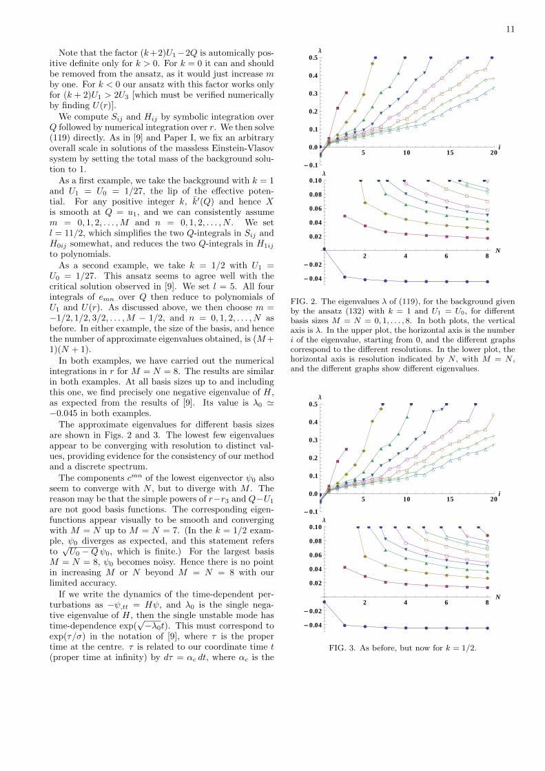
In both examples, we have carried out the numericalintegrations in r for M = N = 8. The results are similarin both examples. At all basis sizes up to and includingthis one, we find precisely one negative eigenvalue of H,as expected from the results of [9]. Its value is λ0 '−0.045 in both examples.

The approximate eigenvalues for different basis sizesare shown in Figs. 2 and 3. The lowest few eigenvaluesappear to be converging with resolution to distinct val-ues, providing evidence for the consistency of our methodand a discrete spectrum.

The components cmn of the lowest eigenvector ψ0 alsoseem to converge with N , but to diverge with M . Thereason may be that the simple powers of r−r3 and Q−U1

are not good basis functions. The corresponding eigen-functions appear visually to be smooth and convergingwith M = N up to M = N = 7. (In the k = 1/2 exam-ple, ψ0 diverges as expected, and this statement refersto√U0 −Qψ0, which is finite.) For the largest basis

M = N = 8, ψ0 becomes noisy. Hence there is no pointin increasing M or N beyond M = N = 8 with ourlimited accuracy.

If we write the dynamics of the time-dependent per-turbations as −ψ,tt = Hψ, and λ0 is the single nega-tive eigenvalue of H, then the single unstable mode hastime-dependence exp(

√−λ0t). This must correspond to

exp(τ/σ) in the notation of [9], where τ is the propertime at the centre. τ is related to our coordinate time t(proper time at infinity) by dτ = αc dt, where αc is the

ææ

æ æ æ æ æ

à

à

à

à

ì

ì

ì

ì

ì

ì

ì

ò

òò

òò

ò

ò

ò

ò

ò

ô

ôô

ôô

ô

ô

ô

ô

ô

ô

ô

ô

ç

çç

çç

çç

ç

çç

ç

ç

ç

ç

ç

ç

ç

á

áá

áá á

áá á

áá

áá

á

áá

á

áá

á

í

íí

í í íí

í íí

íí

íí

íí

íí

í

í í

í

ó

óó ó ó ó

óó ó ó

ó óó

óó

óó

ó ó

ó

óó

5 10 15 20i

- 0.1

0.0

0.1

0.2

0.3

0.4

0.5Λ

æ

ææ æ æ æ æ æ æ

æ æ æ æ æ æ æ æ

à

à

àà à à à à

ì

ì

ìì

ì ì ì

ò

ò

òò

òò

ô

ô

ôô

ô

ç

ç

ç

çç

á

á

á

í

í

ó

ó

õ

2 4 6 8N

- 0.04

- 0.02

0.02

0.04

0.06

0.08

0.10Λ

FIG. 2. The eigenvalues λ of (119), for the background givenby the ansatz (132) with k = 1 and U1 = U0, for differentbasis sizes M = N = 0, 1, . . . , 8. In both plots, the verticalaxis is λ. In the upper plot, the horizontal axis is the numberi of the eigenvalue, starting from 0, and the different graphscorrespond to the different resolutions. In the lower plot, thehorizontal axis is resolution indicated by N , with M = N ,and the different graphs show different eigenvalues.

ææ

æ æ æ æ

à

à

à

à

ì

ì

ì

ì

ì

ì

ì

ì

ò

òò

òò

ò

ò

òò

ò

ò

ô

ôô

ôô ô

ô

ô

ô

ôô

ô

ô

ôô

ç

çç

ç ç çç ç

çç

çç

ç

ç

ç

ç

ç ç

á

áá

á á áá á á

á á

áá

áá

áá

á

áá

á

á

í

íí

í í íí í í í

í í

íí

íí

í íí

íí

í

ó

óó ó ó ó ó ó ó ó ó

ó ó

óó

óó

ó óó

óó

5 10 15 20i

- 0.1

0.0

0.1

0.2

0.3

0.4

0.5Λ

æ

æ æ æ æ æ æ æ æ

æ æ æ æ æ æ æ æ æ

à

à

àà à à à à

ì

ìì

ìì ì ì

ò

ò

òò

òò

ô

ô

ôô

ôô

ç

ç

çç

ç

á

á

áá

í

í

íí

óó

ó

õõ

æ

2 4 6 8N

- 0.04

- 0.02

0.02

0.04

0.06

0.08

0.10Λ

FIG. 3. As before, but now for k = 1/2.

12

lapse at the centre, and hence we have

σ =αc√−λ0

. (136)

With αc ' 0.2968 and λ0 ' −0.0446 for the k = 1 back-ground solution, and αc ' 0.2874 and λ0 ' −0.0445for k = 1/2, the formula (136) gives σ ' 1.41 and1.36, respectively, both compatible with the range σ '1.43± 0.07 given by [9].

However, we have implemented our numerics usingonly standard ODE solvers and nonlinear equationssolvers (for solving the background equations by shoot-ing) and numerical integration and linear algebra meth-ods (for applying the Ritz method to the perturbations)in Mathematica, and have not tried to estimate our nu-merical error or optimise our methods.

V. CONCLUSIONS

Numerical time evolutions of the Einstein-Vlasov sys-tem in spherical symmetry with massless particles [9]have suggested the rather surprising conjecture that allstatic solutions of this system are one-mode unstable,with the time evolutions resulting in collapse for one signof the initial amplitude of this mode, and dispersion forthe other. In the language of critical phenomena in grav-itational collapse, all static solutions are critical solutionsat the threshold of collapse.

In Paper I [7] we have characterised all static solu-tions with massive particles in terms of a single func-tion of two variables k(Q,F ). Here F is essentially con-served angular momentum, and Q essentially conservedenergy per angular momentum, such that the orbit of amassless particle of given Q and F depends on Q alone.Correspondingly, we have the degeneracy that all dis-tributions k(Q,F ) of massless particles with the samek(Q) :=

∫k(Q,F )FdF give rise to the same spacetime.

In the current Paper II we have reduced the pertur-bations of static solutions (in spherical symmetry, witheither massive or massless particles) to a single mastervariable ψ(t, r,Q, F ), which obeys an equation of motionof the form −ψ,tt = (H0 + H1)ψ. In the massless casewe have the same degeneracy for the perturbations as forthe background, that is the metric perturbations only de-pend on ψ =

∫ψ FdF , but in contrast to the background

equations this does simplify the equations significantly.Hence we have assumed m ≥ 0 in most of this paper.

The kinetic part H0 of H is such that ψ,tt = H0ψ issimply a second-order wave equation with characteristicspeeds ±V (r,Q, F ). There is no underlying wave equa-tion in three space dimensions here. Rather, the left andright-going waves correspond to particles moving inwards

and outwards in the background spacetime, with V theirradial velocity.

By contrast, the gravitational part H1 of H vanishes inthe vacuum regions of the background solutions, and con-tains integrals over Q and F (as well as first r-derivatives)representing the gravitational pull of all the other parti-cles represented by the perturbation ψ.

Following a suggestion by Olivier Sarbach, we haveidentified an inner product of perturbations ψ which ispositive definite for suitable background solutions andwith respect to which the operator H is symmetric. Thisadditional mathematical structure allows us to find ap-proximate eigenvectors ψ and eigenvalues λ of H usingthe Ritz method. We have carried out the numerical pro-cedure for two representative background solutions withmassless particles (see Paper I for a discussion of these so-lutions and their significance), and we have found numer-ical evidence for a discrete spectrum of λ with, for bothbackgrounds, a single negative eigenvalue with a valuecompatible with that found by Akbarian and Choptuik[9].

On the analytic side, we have characterised the spaceof functions ψ(r,Q, F ) as V = V ⊕ V, where a certain

integral Iψ over F and Q vanishes for functions in V,while V consists of functions of the form f(r)X(r,Q, F )for a specific X given by the background solution. HenceV is infinitely larger than V. Unfortunately, eigenvectorsψ of H cannot lie entirely in either subspace. We havealso found that we can write H as the difference of twosquares, H = A†A − D†D, with D = D† annihilatingV. Unfortunately, the commutators of A†, A and D arenot simple, and so the apparent analogy with the quan-tisation of the harmonic oscillator does not seem to behelpful.

We had hoped that in bringing the perturbation equa-tions into a sufficiently simple form we could prove theconjecture of [9] that every spherically symmetric staticsolution with massless particles has precisely one unsta-ble mode and/or calculate its value in closed form. Wehad also hoped to be able to show that some sphericallysymmetric static solutions with massive particles are sta-ble, as conjectured in [6]. We have not been able to doeither, but hope that our formulation of the problem willbe of future use.

ACKNOWLEDGMENTS

The author acknowledges financial support fromChalmers University of Technology, and from the Er-win Schrodinger International Institute for Mathematicsof Physics during the workshop “Geometric TransportEquations in General Relativity”. He is grateful to HakanAndreasson for stimulating discussions when this projectwas begun, and to workshop participants Olivier Sar-bach for suggesting the Ritz method and Gerhard Reinfor pointing out [11].

13

[1] G. Rein and A.D. Rendall, Commun. Math. Phys. 150,561 (1992).

[2] M. Dafermos J. Hyperbol. Differ. Equations 3, 589(2006).

[3] J.M. Martın-Garcıa and C. Gundlach, Phys. Rev. D 65,084026, 1 (2002).

[4] A.D. Rendall and J.J.L. Velazquez, Annales HenriPoincare 12, 919 (2011).

[5] G. Rein and A.D. Rendall Math. Proc. Camb. Phil. Soc.128, 363 (2000).

[6] H. Andreasson and G. Rein, Class. Quantum Grav. 23,3659 (2006).

[7] C. Gundlach, Phys. Rev. D 94, 124046 (2016).[8] H. Andreasson, Living Reviews in Relativity 2011-4

(2011).[9] A. Akbarian and M. W. Choptuik, Phys. Rev. D 90,

104023 (2014).[10] J. Schaeffer, Commun. Math. Phys. 204, 313 (1999).[11] H. DeJonghe, Phys. Rep. 133, 217 (1986).