


![Splošno o DSP 1 - studentski.netstudentski.net/get/ulj_fel_el2_dp2_sno_splosno_o_dsp_01.pdf · Diskretna Fourierjeva transformacija ∑ − = = − 1 0 ( ) ( )exp[ (2 / )] N n X](https://static.fdocument.org/doc/165x107/5a7a04e27f8b9ab80d8c949a/splosno-o-dsp-1-fourierjeva-transformacija-1-0-exp-2.jpg)

γλώσσες
Σελίδες
Νομικός


Civil EngineeringSoil Mechanics
& Foundation Engineering
WORKBOOKWORKBOOKWORKBOOKWORKBOOKWORKBOOK
2016
Detailed Explanations ofTry Yourself Questions
© Copyrightwww.madeeasypublications.org
Types and Properties of Soil1
T1 : Solution
Rh′ = 24.5∴ Rh = 24.5 + 0.5 = 25
R = 24.5 – 2.50 = 22
D = ( )����
�
�
�
�
� �
η− γ
where D is in mm, He is in cm and t is in min.For the present case, h = 0.008 × 10⁻⁴ kN-s/m2,
He = 10.7 cm, G = 2.75 and γw = 9.81 kN/m3; t = 30 min
∴ D = ( )�
���� ����� ���������
�� � ����
−× × × =−
� �� �
� �
or D = ������������ ���� �� �� � ������� ��
��
−= ×
The percentage finer is given by
N = ( )���
��
��
� − where Md = mass of dry soil = 50 g
∴ N = ( )��� ����
�� ������� ���� �
×× =
−
T2 : Solution
We have
Activity of clay A = ( )� ����� ����� �� ����
I
© Copyright www.madeeasypublications.org
3Workbook
=�� �
���� �
= = ...(i)
Activity of clay B =( )
( ) �� �� ����� �� ����
� �I
=��
����
=
Since activity of clay A is more than that of clay B, therefore clay A is more likely to undergo high volumechange so clay A has higher compressibility than that of B but permeability and rate of volume change aresmaller than that of clay B.
T3 : Solution
Given ρ = 2.15 mg/m3
(i) ρd =� �
ρ+
= �� ������� ����
� ����=
+
(ii) ρd =�
��
�
ρ+
⇒ 1 + e =���� �
����
�
�
�ρρ
×= = 1.38
⇒ e = 1.38 – 1 = 0.38(iii) Se = wG
S =��
� =
���� ����������
����
×=
⇒ S = 83.59%(iv)Air content, ac = (1 – S)
= 0.1641 = 16.41%
© Copyrightwww.madeeasypublications.org
Classification of Soils2
T1 : Solution
Since more than 50% of the material is larger than 75 μ size, the soil is a coarse grained one.Since more than 50% of coarse fraction is passing sieve 2.032 mm, it is classified as a sand. (This will bethe same as percent passing 4.75 mm sieve)Since more than 12% of the material passes the 75 μ sieve, it must be SM or SC.Now, it can be seen that the plasticity index, Ip is (20 – 12) = 8% which is greater than 7%. Also, if thevalues of wL and Ip are plotted on the plasticity chart, the point falls above A-line.Hence, the soil is to be classified as SC.
T2 : Solution
Plastic index, Ip for soil S1 = wL – wp = (38 – 18) = 20%Ip for soil S2 = wL – wp = (60 – 20) = 40%
Consistency index,
Ic for soil S1 =( ) ( )�� ��
�����
�
� �− −= = −
I
Ic for soil S2 =( )
���
−=
The consistency index for soil S1 is negative, it will become a slurry on remoulding ; therefore, soil S2 islikely to be a better foundation material on remoulding.Flow index, If for soil S1 = 10
If for soil S2 = 5
Toughness index, IT for soil S1 =��
���
= =II

© Copyright www.madeeasypublications.org
5Workbook
IT for soil S2 =��
��
=
Toughness index is greater for soil S2, it has a better strength at plastic limit.
T3 : Solution
(i)(i)(i)(i)(i) Soil A:Soil A:Soil A:Soil A:Soil A: Percent of soil between 4.75 mm and 0.075 mm = 92 – 14 = 78%. Hence the soil is sandy,with a symbol S.Plasticity index = 16 – 8 = 8 > 7. Hence it is clayey sand, SC.
(ii)(ii)(ii)(ii)(ii) Soil B:Soil B:Soil B:Soil B:Soil B: Since more than half is passing 75 micron sieve, it is a fine grained soil.Also Ip = 58 – 14 = 44%.Plotting the point wL = 58% and Ip = 44%, we find that the soil is CH group. Hence soil B is clay ofhigh compressibility.
© Copyrightwww.madeeasypublications.org
Soil Compaction3
T1 : Solution
γt = 19 kN/m3
w = 15%G = 2.7
γt =( )�
��
� �
�
+γ
+
19 =( )�� � ��
����� �
+×
+e = 0.603
Se = wG
S =���� ���
����������
×=
Water content for full saturation
w =�
� = 0.223
Additional water content required for full saturation= 22.33 – 15 = 7.33%
T2 : Solution
Air content, ac = �����
�
�
�=
or, Va = 0.06 Vv,
Hence Vw = 0.94 Vv
© Copyright www.madeeasypublications.org
7Workbook
Thus Va = � ������
⎛ ⎞ =⎜ ⎟⎝ ⎠�
��
�
Volume of specimen, V = ����� ������ ������ ��
π× × = l
Now, V = Vs + Vw + Va2208.9 = Vs + Vw + 0.0638 Vw = Vs + 1.0638 Vw
Writing volume in terms of mass,
2208.9 = ����������� ���� ���
� � ⎛ ⎞+ ⎜ ⎟⎝ ⎠×
Substituting Mw = 0.10 Ms,
2208.9 = ���� �� ����
��
��+ ×
or Ms = 4606.54 gm Mw = 460.65 gmMass of wet soil, M = Ms + Mw = 4606.54 + 460.65 = 5067.19
Bulk density, ρ =�������
����� ����������
�= = l
Dry density, ρd =�����
����� ����� � �����
ρ = =+ +
l
and void ratio, e =���� ���
� � � � ����������
�
�
�ρ ×= =ρ
T3 : Solution
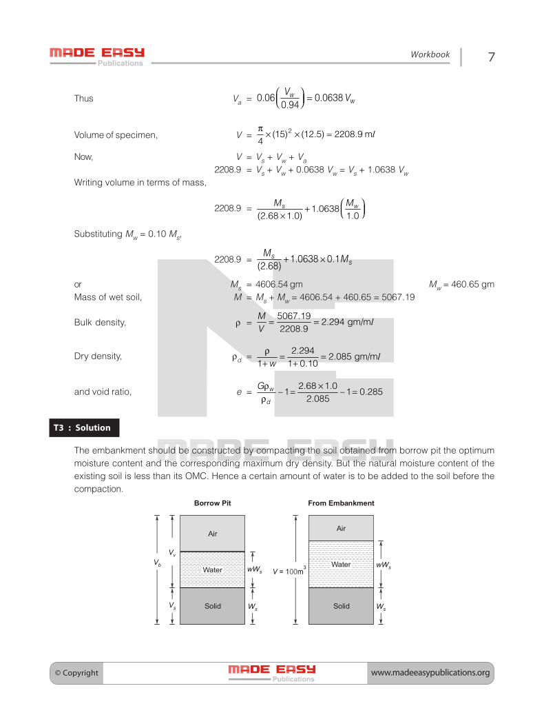
The embankment should be constructed by compacting the soil obtained from borrow pit the optimummoisture content and the corresponding maximum dry density. But the natural moisture content of theexisting soil is less than its OMC. Hence a certain amount of water is to be added to the soil before thecompaction.
Vb
Vv
Vs
wWs
Ws
Air
Solid
Air
Solid Ws
Borrow Pit From Embankment
WaterWater wWs

© Copyrightwww.madeeasypublications.org
8 Civil Engineering • Soil Mechanics & Foundation Engineering
For embankment:For embankment:For embankment:For embankment:For embankment: Data given, (γd ) = 1.66 gm/ccOMC = w = 22.5%
(γd)max = �� �������
�
⎛ ⎞ =⎜ ⎟⎝ ⎠
⇒ Ws = (1.66 × 100) = 166 tonnThe weight of water, Ww = wWs = (0.225 × 166) = 37.35 tonnFor borrow pit area:For borrow pit area:For borrow pit area:For borrow pit area:For borrow pit area:
γt = bulk density = 1.78 gm/cc = 1.78 t/m3
w = 9 %
Therefore, γt = 1.78 = �� �
� ��
�
� �
�
+
⇒ Volume of borrow pit, Vb = ������ ����������� �
����
+ =
∴ Weight of water available from this soilWw = (Ws× w) = (166 × 0.09) = 14.94. tonn.
Therefore quantity of water to be added = (37.35 – 14.94) = 22.41 tonn.γw = 1 gm/cc
= 10–6 tonne/cc = (10–6 × 1000) tonne/lit. = 10–3 tonne/lit.
∴ Volume of water to be added = ��
����� !" #$ �� ��������� %� ��
&��� ' !" #$ �� �= =
T4 : Solution
Data given : Volume of the mould = �� �
�� =
� ����� ��������������
�=
In the loosest state:In the loosest state:In the loosest state:In the loosest state:In the loosest state:
Bulk density, γt = ������� � ���������� �����
������=
Min. Dry density (γd)min. =�����
����� ������ �� �����
�
γ⎛ ⎞ = =⎜ ⎟⎝ ⎠+ +In the densest state:In the densest state:In the densest state:In the densest state:In the densest state:
Bulk density, γ = ������� � ���������� �����
������=
(γd)max =�����
��� ������� ����
=+ ⇒
����������� �����
����=
In-situ density of the soil = 1.61 gm/ccw = 7%
∴ In-situ dry density, γd = ������ �����
�� ��=
+
∴ Relative density, RD = ��( ���
��( ���
� � � � ����
� � � � �� � �
� � �
γ γ γ⎛ ⎞ ×⎜ ⎟γ γ γ⎝ ⎠
=��� ��� ������
� ����� ��� �����
⎛ ⎞ × × =⎜ ⎟⎝ ⎠
© Copyright www.madeeasypublications.org
Effective Stress, Capillarity andPermeability4
T1 : Solution
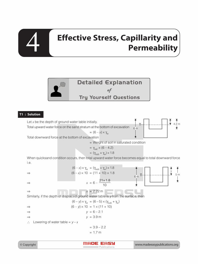
Let x be the depth of ground water table initially.
Total upward water force on the sand stratum at the bottom of excavation
= (6 – x) × γw
Total downward force at the bottom of excavation
= Weight of soil in saturated condition
= γsat × (6 – 4.2)
= (γsub + γw) × 1.8
When quicksand condition occurs, then total upward water force becomes equal to total downward forcei.e.
(6 – x) × γw = (γsub + γw) × 1.8
⇒ (6 – x) × 10 = (11 + 10) × 1.8
⇒ x = 6 – �� ���
��
×
⇒ x = 2.22 m
Similarly, if the depth of displaced ground water table is y from the surface, then
(6 – y) × γw = (6 – 5) × (γsub + γw)
⇒ (6 – y) × 10 = 1 × (11 + 10)
⇒ y = 6 – 2.1
⇒ y = 3.9 m
∴ Lowering of water table = y – x
= 3.9 – 2.2
= 1.7 m
6 m
4.2 mx
6 m5 m
y

© Copyrightwww.madeeasypublications.org
10 Civil Engineering • Soil Mechanics & Foundation Engineering
T2 : Solution
Given
Layer 1
Layer 2
Layer 3
x
x2
4x
k y
k y
k y
1
2
3
=
= 2
= 4
kH = � � ��� ��
� �
� � �+ ++ +
x x xx x x
= � �� ��
� �
� � ��
+ + =x x xx
kV =
� � �
� �
� �
� � �
+ +
+ +
x x xx x x
= �
� �
� �� � �+ +
xx x x
= �
�
�xx
= �
��
�
�
�=
��
��
� �
�
�
�
�
�
=
T3 : Solution
k= �� �� �� �� � ���� �� ����
�� �� ��
� �
� � �
−= × × = ×
Discharge velocity, v= � ������� �� ���� �� ����
��
��� � − −= = × × = ×
l
Seepage velocity, vs=�
��� ������� �� ����
���
�
�
−−×
= = ×
Again �
�
�
�=
( )
( )
�
��� �
� � �
�
�
��
�
�
� �
� �
−+× =
+
−
or, k2=( )
( )
( )
( )
�
� �
� � �
� �
��
�
��
� � ����� �� ��� �� ����
��
� ���
�
− −− −= × × = ×
−−

© Copyright www.madeeasypublications.org
Seepage Analysis5
T1 : Solution
�
�
�∂∂x
= 0
Integrating both sides, we get
�∂∂x
= C1 ...(i)
Integrating againH = C1x + C2
At x = 0, H = 5∴ 5 = C2
At x = 0, ���
�= −
xFrom eq. (i)
C1 = –1∴ H = –x + 5At x = 1.2 m∴ H = 5 – 1.2 = 3.8 m
T2 : Solution
��
� x=
�
�
�� �����
� ��
× =×
D′ = ���� �������
× = ×x

© Copyrightwww.madeeasypublications.org
12 Civil Engineering • Soil Mechanics & Foundation Engineering
D′ = 30.4582 m
S = � � �� � �+′ ′ = � ��������� �� � ������� ��� � �+ =
q = k′S
k ′ = � � �� �� �� �� ���� �� ������ � = × × × = ×x
= 5.366 × 10⁻⁹ m/sq = 5.366 × 10–9 × 3.063 m3/s/m = 16.438 × 10⁻⁹ m3/s/m
Total head = 14 m
Total head at x =�
�� � �� ���� ���
× =
Total head = Pressure head + elevation head
⇒ 11.67 = ��
� +γx
⇒�
�
γx
= 5.67 m
Px = 5.67 γw = 56.7 kN/m2
T3 : Solution
From the Figure,Nf = No. of Flow channels = 5Nd = No. of Head drop = 16
∵ K = 0.015 cm/sec = ������ ��
����� ��)$'�
�����
×=
⎛ ⎞⎜ ⎟⎝ ⎠
H = 5 m
∴ q = ������ ���� � �)$' ��
���
�
���
�
⎛ ⎞ ⎛ ⎞= × =⎜ ⎟⎜ ⎟ ⎝ ⎠⎝ ⎠
∴ Total quantity of seepage loss per day = q × Width = 20.25 × 55 = 1113.75 m3/dayThe avg. length of smallest flow element adjacent to the weir = 1.2 m.
∴ Exist Gradient, ie =�
����� ���
� �
�
Δ ⎛ ⎞ ⎛ ⎞= = =⎜ ⎟⎜ ⎟ ⎝ ⎠× ×⎝ ⎠l l
Critical Hydraulic Gradient, ic =�� ��� ��
���� � ����
�
�
⎛ ⎞ ⎛ ⎞= =⎜ ⎟ ⎜ ⎟⎝ ⎠ ⎝ ⎠+ +
∴ Factor of safety against piping =���
������
�
= =ii
© Copyright www.madeeasypublications.org
13Workbook
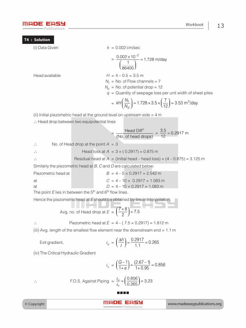
T4 : Solution
(i) Data Given k = 0.002 cm/sec
= ����� ��
���� ������
�����
× =⎛ ⎞⎜ ⎟⎝ ⎠
Head available H = 4 – 0.5 = 3.5 mNf = No. of Flow channels = 7Nd = No. of potential drop = 12q = Quantity of seepage loss per unit width of sheet piles
= ����� �� ��� � �)$'
���
�
���
�
⎛ ⎞ ⎛ ⎞= × × =⎜ ⎟⎜ ⎟ ⎝ ⎠⎝ ⎠
(ii) Initial piezometric head at the ground level on upstream side = 4 m
∴ Head drop between two equipotential lines
=�*��� ����
�+� �� ���� ���,�� =
������� �
��=
∴ No. of Head drop at the point A = 3
∴ Head loss at A = 3 × ( 0.2917) = 0.875 m
∴ Residual head at A = (Initial head – head loss) = (4 – 0.875) = 3.125 m
Similarly the piezometric head at B, C and D are calculated below:
Piezometric head at B = 4 – 5 × 0.2917 = 2.542 m
at C = 4 – 10 × 0.2917 = 1.083 mat D = 4 – 10 × 0.2917 = 1.083 mThe point E lies in between the 5th and 6th flow lines.
Hence the piezometric head at E should be obtained by linear Interpolation.
Avg. no. of Head drop at E = �
��
+⎛ ⎞ =⎜ ⎟⎝ ⎠
∴ Piezometric head at E = 4 – ( 7.5 × 0.2917) = 1.812 m
(iii) Avg. length of the smallest flow element near the downstream end = 1.1 m
Exit gradient, ie =�����
�������
�Δ⎛ ⎞ = =⎜ ⎟⎝ ⎠l
(iv) The Critical Hydraulic Gradient
ic =�� ���� ���
����� � ���
�
�
⎛ ⎞ = =⎜ ⎟⎝ ⎠+ +
∴ F.O.S. Against Piping =����
�������
�
⎛ ⎞= =⎜ ⎟⎝ ⎠ii
© Copyrightwww.madeeasypublications.org
Stress Distribution in Soils6
T1 : Solution
We know that, σz =( )
� � ���
� �
� � �
�
� ! �
×π ⎡ ⎤+⎣ ⎦
Point P, r/z = 0 σz = �
� � � �
� ���� ������ -+��
� ��� .� �/
× × =π +
Point R, r/z = 5/6 σz =( )
�
� � � � �
� ���� ����-+��
� ��� .� � � � /
× × =π +
T2 : Solution
We know that σz =( )
�
�
� �
� �
"
� �
⎡ ⎤⎢ ⎥
π ⎢ ⎥+⎣ ⎦x
At point P, σz =( )
�
�
� ��� �
��� � �����
⎡ ⎤× ⎢ ⎥π × ⎢ ⎥+⎣ ⎦
= 12.40 kN/m2
© Copyright www.madeeasypublications.org
Compressibility andConsolidation7
T1 : Solution
#σ′ =�
�� �σ σ′ ′
σ′ = ( )��# �σ σ′ ′
Where,��
σ′ = Effective stress at the level under consideration,
For sample A
2 m
7.0 m
γ = 18.3 kN/m3
γ = 19.0 kN/m3
4 m
��σ′ = (2 × 18.3) + (19 – 10) × 2 = 54.6 kN/m2
∴ #σ′ = ( )�� ����� ����� �σ σ =′ ′ = 46.4 kN/m2
∴ At the centre of first layer effective stress before application of proposed fill
�σ′ = 2 × 18.3 + 3.5 × (19 – 10) = 68.1 kN/m2
∴ �Δσ′ = After placing the proposed fill
= (8.5 × 20.3) = 172.55 kN/m2
∴ Final stress at centre = ( )� �σ + Δσ′ ′ = (68.1 + 172.55) = 240.65 kN/m2
Pre consolidation stress at the point = ( )��σ + σ′ ′ = 68.1 + 46.4
��σ′ = 114.5 kN/m2
© Copyrightwww.madeeasypublications.org
16 Civil Engineering • Soil Mechanics & Foundation Engineering
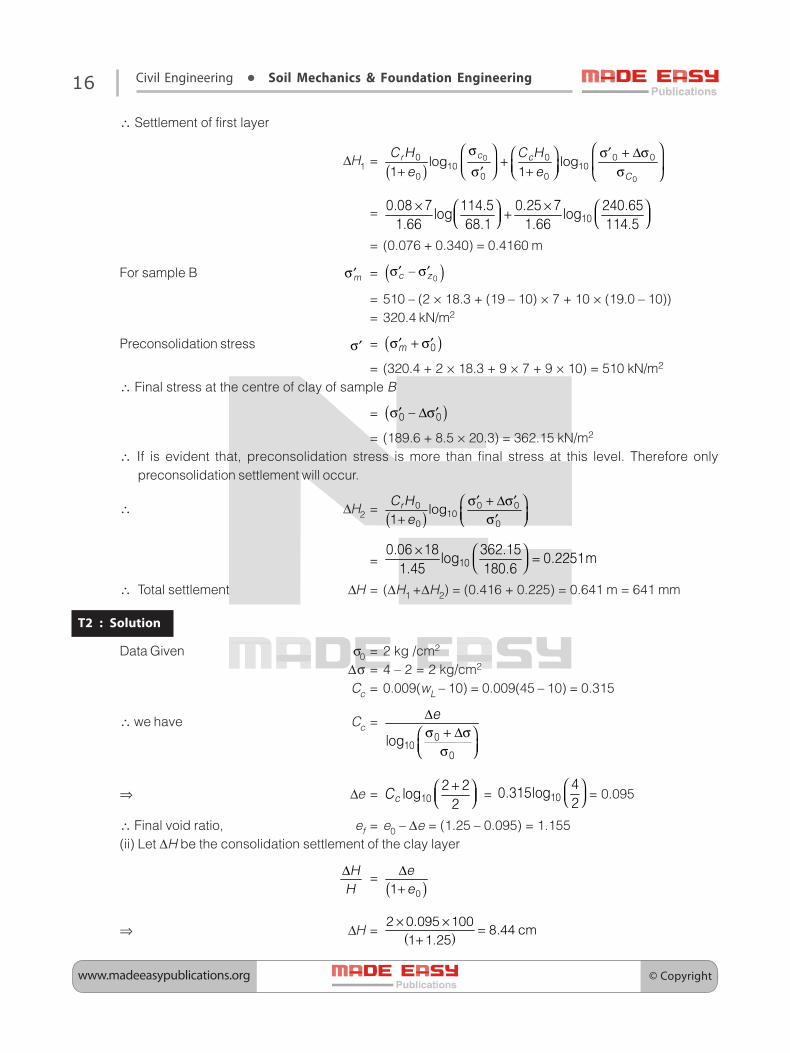
∴ Settlement of first layer
ΔH1 =( )
�
�
� � � ��� ��
� � �
��� ���� �
�
$
$ � $ �
� �
⎛ ⎞σ⎛ ⎞ σ′ + Δσ⎛ ⎞+ ⎜ ⎟⎜ ⎟ ⎜ ⎟+ σ + σ′⎝ ⎠ ⎝ ⎠ ⎝ ⎠
=��
���� ���� ��� �����%!� %!�
���� ���� ���� ����
× ×⎛ ⎞ ⎛ ⎞+⎜ ⎟ ⎜ ⎟⎝ ⎠ ⎝ ⎠
= (0.076 + 0.340) = 0.4160 m
For sample B #σ′ = ( )�� �σ σ′ ′
= 510 – (2 × 18.3 + (19 – 10) × 7 + 10 × (19.0 – 10))= 320.4 kN/m2
Preconsolidation stress σ′ = ( )�σ + σ′ ′�
= (320.4 + 2 × 18.3 + 9 × 7 + 9 × 10) = 510 kN/m2
∴ Final stress at the centre of clay of sample B
= ( )� �σ Δσ′ ′
= (189.6 + 8.5 × 20.3) = 362.15 kN/m2
∴ If is evident that, preconsolidation stress is more than final stress at this level. Therefore onlypreconsolidation settlement will occur.
∴ ΔH2 = ( )� � �
��� �
����
�� �
�
σ + Δσ′ ′⎛ ⎞⎜ ⎟+ σ′⎝ ⎠
= ������ �� ����
%!� ��������� �����
× ⎛ ⎞ =⎜ ⎟⎝ ⎠
∴ Total settlement ΔH = (ΔH1 +ΔH2) = (0.416 + 0.225) = 0.641 m = 641 mm
T2 : Solution
Data Given σ0 = 2 kg /cm2
Δσ = 4 – 2 = 2 kg/cm2
Cc = 0.009(wL – 10) = 0.009(45 – 10) = 0.315
∴ we have Cc =�
���
%!�
�Δσ + Δσ⎛ ⎞
⎜ ⎟σ⎝ ⎠
⇒ Δe = ��� �
%!��
��+⎛ ⎞
⎜ ⎟⎝ ⎠ = ���
���%!��
⎛ ⎞⎜ ⎟⎝ ⎠ = 0.095
∴ Final void ratio, ef = e0 – Δe = (1.25 – 0.095) = 1.155(ii) Let ΔH be the consolidation settlement of the clay layer
�
�
Δ =( )��
�
�
Δ+
⇒ ΔH = ( )� � ��� ���
� �� ��� � ��
× × =+

© Copyright www.madeeasypublications.org
17Workbook
(iii) In the pressure range of 2 to 4 kg/cm2
mv =�
� ��� �
�� � �� � ��� �
�
�
Δ = ×+ × Δσ +
= 0.021 cm2/kg∵ k = 2.8 × 10⁻⁷ cm/sec
γw = 1 gm/cc = 10–3 kg/cc
∴ Cv = ( )� �
�
γ = ��
���
��� �������� �� ����
������ �� �
× =×
For 50% consolidation T50 = ( )�� � � ����
π =
∴ t =
�
����
� ���� ���
� �����
�
% �
�
⎛ ⎞× ⎜ ⎟⎝ ⎠=
t = 148120.3008 sec = 1.71 days
T3 : Solution
Raft
9.2 t/m2 1.2 m2 m
8 m
6 m
Sub layer - I
Sub layer - II
Sub layer - III
Clay
e G0 = 0.72, = 2.71
w CL v = 42%, = 2.2 × 10 cm /sec–3 2
Sand
γ = 1.90 t/m3
d
γ = 2.10 t/m3
sat
Impervious shale
G.L.
The clay layer is divided into three sub layers of thickness 2 m each.For the settlement of each layer
We have ΔH = ( )� �
� �
����
� �
�
σ + Δσ⎛ ⎞⎜ ⎟+ σ⎝ ⎠
The computation of settlement for the first sub layerCc = 0.009 (wL – 10)Cc = 0.009 (42 – 10) = 0.288e0 = 0.72H0 = 2m = 200 cm

© Copyrightwww.madeeasypublications.org
18 Civil Engineering • Soil Mechanics & Foundation Engineering
∴ Depth of middle of the sub-layer-I below:
GL = �
� � ��
+ =
σ0 = Initial effective overburden stress at a depth of 9 mbelow G.L
= (γd h1 + γsub h2+ γclay h3)γsat = 2.10 t/m3 ; γw = 1.0 t/m3
∴ γsub = (2.10 – 1.0) = 1.10 t/m3
γclay = �� � ���� ���� ���� ��
�� � �� ������ �
�
+ γ + ×= =
+ +
∴ σ0 = 1.9 × 2 + 1.10 × 6 + (2 – 1) × 1 = 11.4 t/m2 = 1.14 kg/cm2
Using 2 : 1 Dispersion Method
q = 9.2 t/m2
Z = (9 – 1.2) = 7.8 m
21
Z / 2 Z / 2L
Δσ =� �� �
��
� & &+ +
= � ���� �� ����� �� ��� �����
��� ��� ���� ���
× × = =+ × +
∴ ΔH1 = ��
� ��� ��� � �� � ������ � �� ��
�� � ��� � ��
× +⎛ ⎞ =⎜ ⎟⎝ ⎠+
Similarily for second layer
q = 9.2 t/m2
Z = (11 – 1.2) = 9.8 m
σ0 = (γdh + γsub h2 + γclay h3) = ( 1.9 × 2 + 1.10 × 6 + 1× 3) = 13.4 t/m2 = 1.34 kg/cm2
Δσ =� �� �
��
� & &+ +

© Copyright www.madeeasypublications.org
19Workbook
=��� ��� ��
���� ������� ����
× ×+ +
= 2.48 t/m2 = 0.248 kg/cm2
ΔH2 = ��
� ��� ��� � �� � ������ � �� ��
�� � ��� � ��
× +⎛ ⎞ =⎜ ⎟⎝ ⎠+
Similarly for Third sub layer σ0 = (γd h1 + γsub h2 + γclay h3)= (1.9 × 2 + 1.1 × 6 + 1 × 5) = 15.4 t/m2 = 1.54 kg/cm2
Δσ =� �� �
��
� & &+ +
=��� ��� ��
���� ����� ��� �����
× ×+ + +
= 2.06 t/m2 = 0.206 kg/cm2
Δh3 = ��
� ��� ��� � �� � ������ � �� ��
�� � ��� � ��
× +⎛ ⎞ =⎜ ⎟⎝ ⎠+
∴ Probable settlement of the clay layerΔH = (ΔH1 + ΔH2 + ΔH3) = (3.45 + 2.47 + 1.83) = 7.75 cm
(ii) Degree of consolidation corressponding to a settlement of 5 cm
U =�
��� �� ���� ��
× =
The corresponding time factor
Tv = 1.781 – 0.933 log10 (100 – 64.52)
Tv = 0.335
As single drainage condition prevails at site
t =( )
( )��
� � ���
� � ��
�
�
% �
� −
⎛ ⎞ ×=⎜ ⎟⎝ ⎠ ×
= 634 days

© Copyrightwww.madeeasypublications.org
Shear Strength of Soils8
T1 : Solution
Undisturbed state
τf = c
τ
0 qu σ
Initial Area of cross section of the sample,
A0 = � ��� ��� �� �� ���
π =
Axial strain at failure, ε0 =
Δ⎛ ⎞⎜ ⎟⎝ ⎠
ε0 = �������
�
⎛ ⎞ =⎜ ⎟⎝ ⎠
7.5 cm
P = 116.3 kg
3.75 cm
∴ Corrected area, Ac = ( ) ( )��
�
�� ���� �� ��
�� �� � ��
�= =
ε
∴ Normal stress at failure = ���� �� �� -����
�� ��
�
�
⎛ ⎞ ⎛ ⎞= =⎜ ⎟⎜ ⎟ ⎝ ⎠⎝ ⎠
∴ Unconfined compressive strength, qu = 9.27 kg/cm2
and Cohesion, c = ������� �����
� �'�⎛ ⎞ ⎛ ⎞= =⎜ ⎟ ⎜ ⎟⎝ ⎠ ⎝ ⎠
© Copyright www.madeeasypublications.org
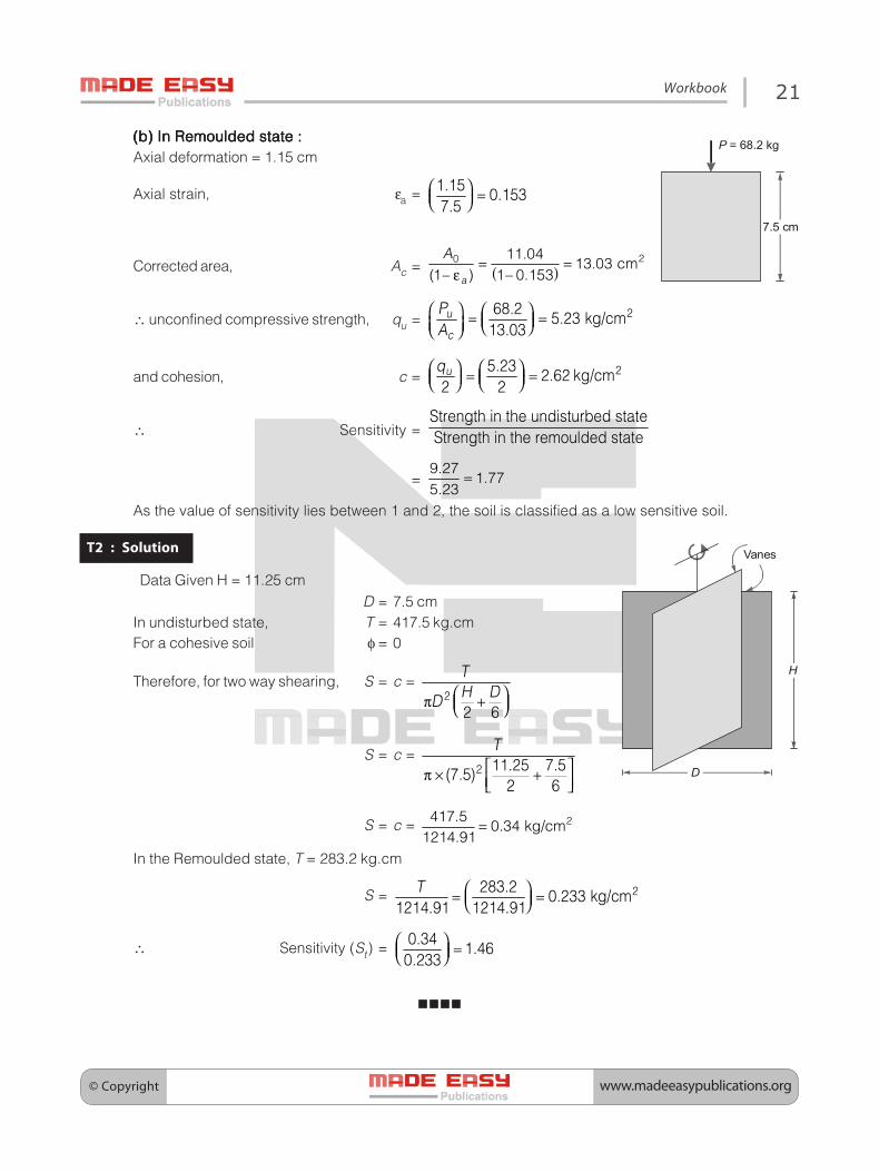
21Workbook
(b) In Remoulded state :(b) In Remoulded state :(b) In Remoulded state :(b) In Remoulded state :(b) In Remoulded state :Axial deformation = 1.15 cm
Axial strain, εa = ������
�
⎛ ⎞ =⎜ ⎟⎝ ⎠
7.5 cm
P = 68.2 kg
Corrected area, Ac = ( )�� �� ��
�� �� ����� � �� � ����
�= =
ε
∴ unconfined compressive strength, qu = ������� �����
���'
�
�
�
⎛ ⎞ ⎛ ⎞= =⎜ ⎟⎜ ⎟ ⎝ ⎠⎝ ⎠
and cohesion, c = ������� �����
� �'�⎛ ⎞ ⎛ ⎞= =⎜ ⎟ ⎜ ⎟⎝ ⎠ ⎝ ⎠
∴ Sensitivity =0 ���� � �� �� 1�)�� 1�2�) � $ �
0 ���� � �� �� ���!1%)�) � $ �
=� ��
� ��� ��
=
As the value of sensitivity lies between 1 and 2, the soil is classified as a low sensitive soil.
T2 : Solution
Data Given H = 11.25 cm
H
D
Vanes
D = 7.5 cmIn undisturbed state, T = 417.5 kg.cmFor a cohesive soil φ = 0
Therefore, for two way shearing, S = c = �
� �
�
� ��
⎛ ⎞π +⎜ ⎟⎝ ⎠
S = c = � ���� �
���� �
�
⎡ ⎤π × +⎢ ⎥⎣ ⎦
S = c = ���� �� �� -����
���� ��=
In the Remoulded state, T = 283.2 kg.cm
S = �������� �����
������� �������
� ⎛ ⎞= =⎜ ⎟⎝ ⎠
∴ Sensitivity (St) = �������
���
⎛ ⎞ =⎜ ⎟⎝ ⎠
© Copyrightwww.madeeasypublications.org
T1 : Solution
K0 = 1 – sin φ = 1 – sin 30° = 0.50At point B, �σ = 2 × 17 = 34 kN/m2, u = 0
p0 = K0 �σ = 0.5 × 34 = 17 kN/m2
At point C, �σ = 2 × 17 + 19 × 2 = 72 kN/m2
p0 = K0 �σ = 0.5 × 72 = 36 kN/m2
The pressure distribution diagram is shown below, the diagram has been divided into 3 parts, let P1, P2 andP3 be the total pressure due to these parts. Thus
(1)
(2) (3)
17.0 kN/m2
19.0 kN/m2
P1 =�
�� ��
× × = 17 kN
P2 = 2 × 17 = 34 kN
P3 = ��� �
�× × = 19 kN
Total, P = P1 + P2 + P3 = 70 kNThe line of action of P is determined by taking moments about C.
∴ � =�� � �� �� � � �� � ��
��
× + × + ×
= 1.32m (from base)
T2 : Solution
Sand silty layer
pa = � �� �� � � �γ
at Z = 0, pA = � � �� �
Lateral Earth Pressure andRetaining Walls9
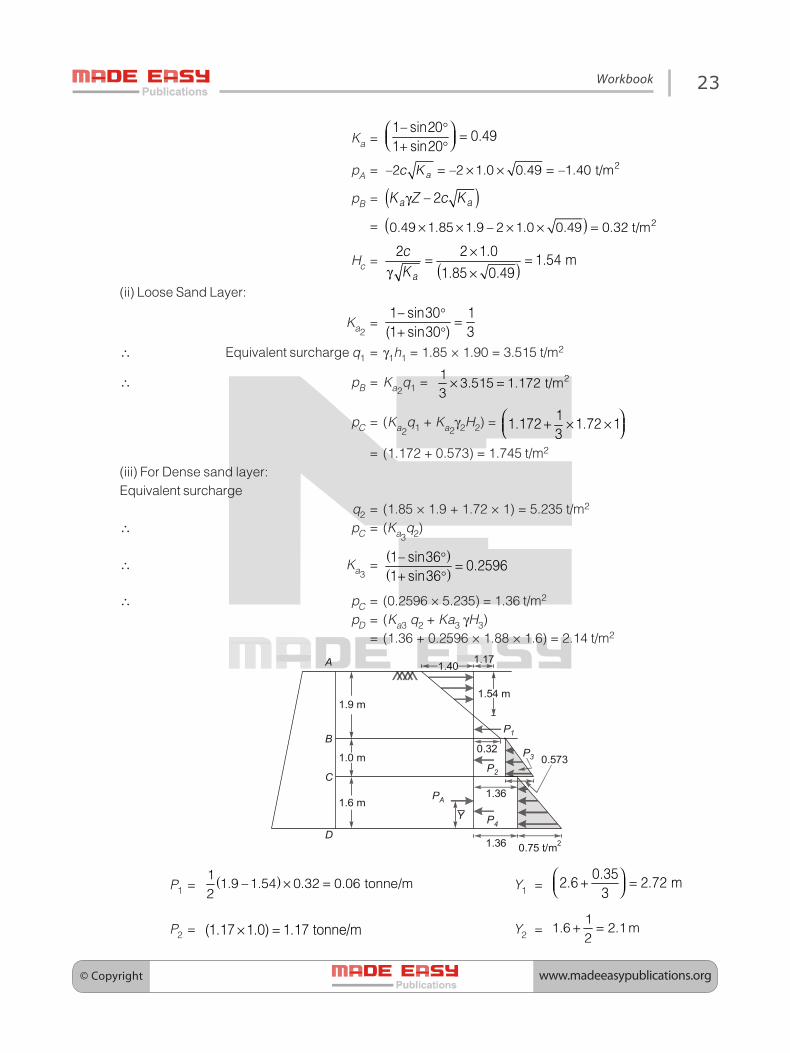
© Copyright www.madeeasypublications.org
23Workbook
Ka =�� �����
����� �����
°⎛ ⎞ =⎜ ⎟⎝ ⎠+ °
pA = ��� �� � � � �� �� �� ����� � = × × =
pB = ( ) �� �� � �γ
= ( ) ����� ���� ��� � � ��� ���� ���� ���× × × × =
Hc = ( )� � �
�� ��� ���
×= =
γ ×�
�
�
(ii) Loose Sand Layer:
Ka2=
� ���
� ��� � �
°=
+ °∴ Equivalent surcharge q1 = γ1h1 = 1.85 × 1.90 = 3.515 t/m2
∴ pB = Ka2q1 = ��
����� ����� ����
× =
pC = (Ka2q1 + Ka2
γ2H2) = �� ��
�
⎛ ⎞+ × ×⎜ ⎟⎝ ⎠= (1.172 + 0.573) = 1.745 t/m2
(iii) For Dense sand layer:Equivalent surcharge
q2 = (1.85 × 1.9 + 1.72 × 1) = 5.235 t/m2
∴ pC = (Ka3q2)
∴ Ka3=
( )( )� ����
���� ����
°=
+ °
∴ pC = (0.2596 × 5.235) = 1.36 t/m2
pD = (Ka3 q2 + Ka3 γH3)= (1.36 + 0.2596 × 1.88 × 1.6) = 2.14 t/m2
A
B
C
D
PA1.6 m
1.0 m
1.9 m
Y P4
1.36
P20.573P3
0.32
P1
1.54 m
1.171.40
1.36 0.75 t/m2
P1 = ( )���� � ���� ���� ���� �������
�× = Y1 =
����� ��� �
�
⎛ ⎞+ =⎜ ⎟⎝ ⎠
P2 = �� � �����× = Y2 =�
��� ��� ��
+ =
© Copyrightwww.madeeasypublications.org
24 Civil Engineering • Soil Mechanics & Foundation Engineering
P3 = ( )������ � ������ �������
�× × = Y3 =
�� ��� �
�
⎛ ⎞+ =⎜ ⎟⎝ ⎠
P4 = ���� ��� ��� !�����× = Y4 =���
��� ��
=
P5 =�
���� ��� ���� ��������
× × = Y5 =���
�����
=
∴ PA = � � � � ��
� � ��� !������
� =
= + + + + =∑ ii
∴ ( =( )� � � � � �
�� � � � � � � � �
�
+ + + +
=����� ���� ���� ��� ������ ���� ���� ��� ���� �����
����
× + × + × + × + ×
! = 1.21 m
∴ The point of application of PA = 4.30 tonne is located at 1.21 m above the base of the wall.
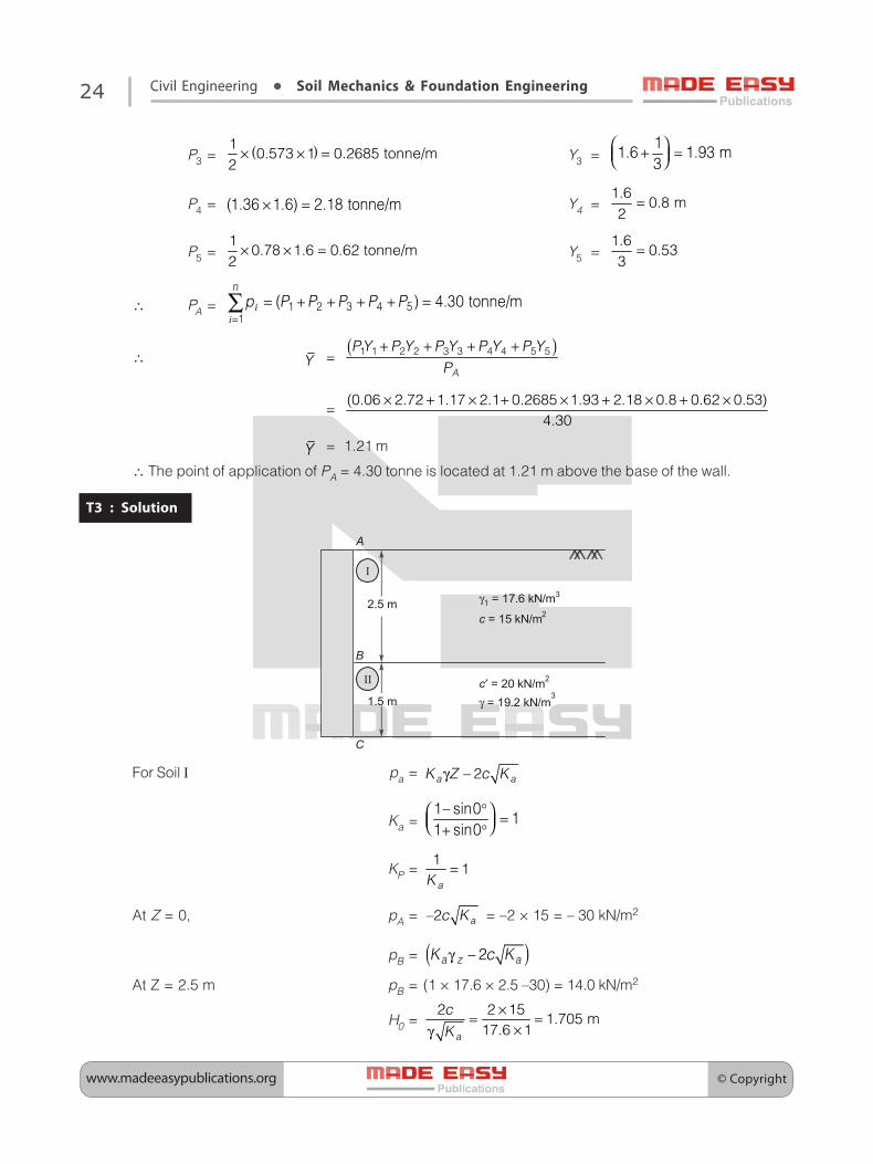
T3 : Solution
A
B
C
2.5 m
1.5 m
γ1 = 17.6 kN/m
= 15 kN/m
3
2c
= 20 kN/mc′ 2
γ = 19.2 kN/m3
I
II
For Soil I pa = � �� �� � � �γ
Ka =� ��
��
°⎛ ⎞ =⎜ ⎟⎝ ⎠+ °
KP =�
���
=
At Z = 0, pA = �� �� � = –2 × 15 = – 30 kN/m2
pB = ( ) �� � �� � �γ
At Z = 2.5 m pB = (1 × 17.6 × 2.5 –30) = 14.0 kN/m2
H0 =� � ��
����� ����� �
�
�
�
×= =×γ

© Copyright www.madeeasypublications.org
25Workbook
For soil III
Ka2=
� ���
��
°⎛ ⎞ =⎜ ⎟⎝ ⎠+ °Equivalent surcharge q = γh = (17.6 × 2.5) = 44 kN/m2
pb = ( )� �� �� �� � � �′ = (1 × 44 – 2 × 20) = 4 kN/m2
At point C pc = ( )� �� � � �� � �� �� � �γ + γ ′
= � ����� ��� ���� ���� � � � �× × + × ×
= 44 + 28.8 – 40 = 32.8 kN/m2
4 kN/m2
b cd
–
a
A
B
C
2.5 m
1.5 m
14 kN/m2
f
32.8 m kN/m2
e
–30 kN/m2
The total active thrust when crack has developed
PA = � ����
��� �� �� �
+× × + × = 33.165 kN/m
T4 : Solution
γ = 16 kN/m3, φ = 35°, δ = 10°, θ = 90° – 85° = 5°, β = 0
Ka =
�
�� ��� �
���� ����� � ��� �
��� �
⎡ ⎤⎢ ⎥θ φ − θ⎢ ⎥⎢ ⎥φ + δ φ − βθ + δ +⎢ ⎥β − θ⎢ ⎥⎣ ⎦
=
�
�� � ����� � �
������ �� ������� � � ���� �� �
���� � �
⎡ ⎤⎢ ⎥° ° − °⎢ ⎥⎢ ⎥° + ° ° − °° + ° +⎢ ⎥° − °⎢ ⎥⎣ ⎦
= 0.2877
Pa = � ��
� �3 * ������ �� ���
� �γ = × × × = 57.54 kN/m
© Copyrightwww.madeeasypublications.org
Stability of Earth Slopes10
T1 : Solution
Data Givenβ = 35°, H = 15 m, φ = 15°, c = 200 kN/m2, γ = 18 kN/m3, Sn = 0.06
We know that Sn = #�
�
⎛ ⎞⎜ ⎟⎝ γ ⎠
⇒ 0.06 =�
��
×cm = (0.06 × 18 × 15) = 16. 2 kN/m2
Factor of safety w.r.t cohesion
FC =���
���������#
�
�
⎛ ⎞ ⎛ ⎞= =⎜ ⎟⎜ ⎟ ⎝ ⎠⎝ ⎠
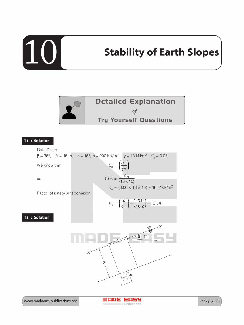
T2 : Solution
X
Y
X
Y
Z
b
αβ
σZ
β = 6°

© Copyright www.madeeasypublications.org
27Workbook
Effective stress at point, σ = (γsub Z cos2β)
Shear stress at at point, τ = γsatZ cosβ sinβShear strength of the soil on Y–Y
τf = ( ) ( )�� � ��� � �����σ φ + = γ β φ
∴ Factor of safety, F = �τ⎛ ⎞⎜ ⎟⎝ ⎠τ
F =��!� $�
�!� ����'�
���
&
&
γ β φγ β β
= � ��� �
� ��� ����
��
γ φγ β
Data Given : β = 16°G = 2.70e = 0.72φ = 35°
γsub = �
��
�
γ+
∴ γsub = ��� � ���� ��
��
× =+
γsat = ( )� �� ��
��� �� ��
�� �
�
+ γ + ×= =+ +
∴ F =���� $��
����� $��
× =× °
© Copyrightwww.madeeasypublications.org
T1 : Solution
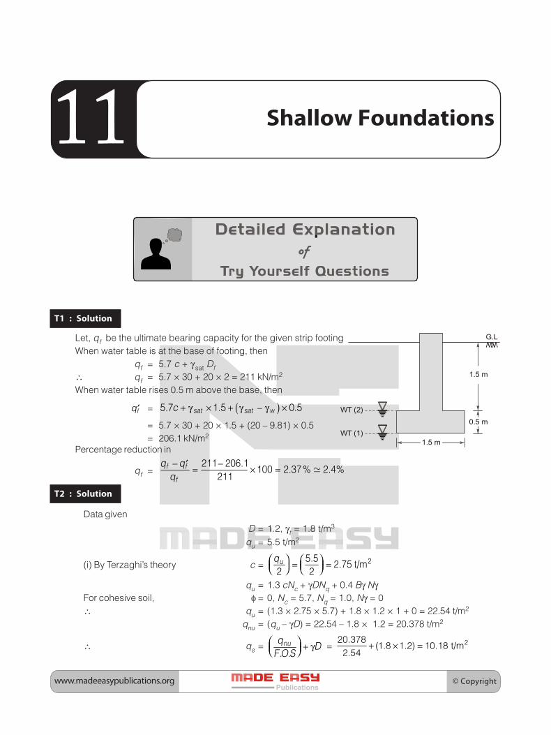
0.5 m
1.5 m
1.5 m
WT (2)
WT (1)
G.LLet, qf be the ultimate bearing capacity for the given strip footingWhen water table is at the base of footing, then
qf = 5.7 c + γsat Df∴ qf = 5.7 × 30 + 20 × 2 = 211 kN/m2
When water table rises 0.5 m above the base, then
" ′ = ( )� � ���� ��� �� + γ × + γ − γ ×
= 5.7 × 30 + 20 × 1.5 + (20 – 9.81) × 0.5= 206.1 kN/m2
Percentage reduction in
qf =� ���
���� �����
� �
�
� �
�
− −′= × = �
T2 : Solution
Data given
D = 1.2, γt = 1.8 t/m3
qu = 5.5 t/m2
(i) By Terzaghi’s theory c = ���� ��
� �'�⎛ ⎞ ⎛ ⎞= =⎜ ⎟ ⎜ ⎟⎝ ⎠ ⎝ ⎠
qu = 1.3 cNc + γDNq + 0.4 Bγ NγFor cohesive soil, φ = 0, Nc = 5.7, Nq = 1.0, Nγ = 0∴ qu = (1.3 × 2.75 × 5.7) + 1.8 × 1.2 × 1 + 0 = 22.54 t/m2
qnu = (qu – γD) = 22.54 – 1.8 × 1.2 = 20.378 t/m2
∴ qs =� ��'�
�)*+
⎛ ⎞ + γ⎜ ⎟⎝ ⎠ = ����������� ���� ����� ���
����+ × =
Shallow Foundations11

© Copyright www.madeeasypublications.org
29Workbook
(ii) By Skempton’s Theory
�
�
⎛ ⎞⎜ ⎟⎝ ⎠
=��
��� ����
⎛ ⎞ = <⎜ ⎟⎝ ⎠
∴ Nc = � � ��� �
⎡ ⎤⎛ ⎞+ ⎜ ⎟⎢ ⎥⎝ ⎠⎣ ⎦ = ��
� �� �����
⎡ ⎤+ × =⎢ ⎥⎣ ⎦∴ qnu = cNc = 2.75 × 6.576 = 18.084 t/m2
∴ qu = qnu + γD = 18.084 + 1.8 × 1.2 = 20. 244 t/m2
∴ qs =� � ��'
��
�)*+
⎛ ⎞ + γ⎜ ⎟⎝ ⎠ = ������� �� ���� ��
���
⎛ ⎞+ × =⎜ ⎟⎝ ⎠
T3 : Solution
1 m1.5 m
X X
2 m
2 m
Δp
12
(i) Computation of bearing capacityqnu = cNc
∴ �
=
������� ���
�= <
∴ Nc = �� ��
� �
� �
+⎛ ⎞ ⎛ ⎞+ +⎜ ⎟ ⎜ ⎟⎝ ⎠ ⎝ ⎠
=�� �
� �
×⎛ ⎞+⎜ ⎟⎝ ⎠ = 6.9
∴ qnu = cNc = 6.9 × 3 = 20.7 t/m2
∴ For a F.O.S of 2.5, the net safe bearing capacity is given by
qns = ��������� ���
� � � � �����"
� ��
⎛ ⎞= =⎜ ⎟⎝ ⎠
qs = 8.28 + 1.8 × 1.5 = 10.98 t/m2
Computation of SettlementAs the underlaying soil is saturated silty clay, only consolidation settlement will take place.
• The zone of influence below the base of footing is extended to maximum depth of twice the width offooting, i.e. 4 m below the base.
• X – X is a horizontal plane through the middle of thin consolidation layer.
© Copyrightwww.madeeasypublications.org
30 Civil Engineering • Soil Mechanics & Foundation Engineering
(σ0)XX = (γ z1 + γsub z2)
= (1.8 × 1.0) + (1.8 – 1) × (0.5 + 2.0) = 3.8 t/m2 = 0.38 kg/cm2
using 2 : 1 dispersion method, stress increament at X – X
(Δσ)XX =�
������ ��� ����
���� ����
× ×+
Assuming the footing to be loaded with 8.28 t/m2 and
= 2.745 t/m2 = 0.2745 kg/cm2
∴ ΔH = � ���
� �
%!��
�� �
�
σ + Δσ⎛ ⎞⎜ ⎟+ σ⎝ ⎠
= ��
��� ����� ���� ��������� ����� �
�� ����� ����
× +⎛ ⎞ =⎜ ⎟⎝ ⎠+
As the Estimated Settlement is greater than the maximum permissible limit of 7.5 cm. The allowablebearing capacity of the footing should be less then 10.98 t/m2
∴ ����
� �
� ����
�� �
,,� �
�
σ + Δσ⎛ ⎞⎜ ⎟+ σ⎝ ⎠ = 7.5
⇒ ��
��� ����� �������
�� ����� ����
× + Δσ⎛ ⎞⎜ ⎟⎝ ⎠+
= 7.5
⇒ ����
����
+ Δσ = 1.3612
⇒ Δσ = 0.1372 kg/cm2 = 1.372 t/m2
⇒ Δσ =�
� �
�
� �
��� ��� �
� & � & � &
×= =+ + + +
⇒ 1.372 =�
��
" ×
⇒ q = (1.372 × 4) = 5.49 t/m2
Hence a loading intensity of 5.49 t/m2 will result in a consolidation settlement of 7.5 cm. Therefore, therequired allowable bearing capacity of the footing = 5.49 t/m2

© Copyright www.madeeasypublications.org
T1 : Solution
Qg(u) = qp Ag + α c(Pg D)= (9 × 100) (1.8 × 1.8) + 1 × 100 × (4 × 1.8 × 10)
or Qug = 10116 kNQu = qpAp + α c(p × D)
= (9 × 100) × π/4 × (0.3)2 + 0.6 × 100(π × 0.3) × 10or Qu = 629.1 kN
Qug = nQu
= 9 × 629.1 = 5661.9 kNAs the ultimate load for individual pile failure is less than the pile groupload, the safe load is given by
Qn =������
������ -+�
=
T2 : Solution
From the Modified Hiley’s FormulaWe know that, the Ultimate load on pile
Qu =( )� ���
� ���
� �
η η+
. . . (i)
Where ηh = Efficiency of hammer = 75% = 0.75W = 2.0 tonneH = 91 cm
Deep Foundations12
����
��
�����
�����
������ ������
����
����

© Copyrightwww.madeeasypublications.org
32 Civil Engineering • Soil Mechanics & Foundation Engineering
S = Avg. penetration under the last 5 blows = 10 mm = 1cmeP = 0.55 × 1.5 = 0.825 tonne
∵ W > eP
⇒ ηb =� �� ������ ���
������ � �� ����
� � �
� �
+ + ×= =+ +
In order to find out the value of Qu, assume as a first approximation,C = 2.5 cm
∴ Qu =���� � �� �����
����� ������ ��� � ��� ��
� ���
� �
η η × × ×⎛ ⎞= =⎜ ⎟⎝ ⎠+ +
Now using C1 =�
����� � �� ��
��
'
"
�
⎛ ⎞ = × =⎜ ⎟ π⎝ ⎠
C2 =�
���� ���� �� ����
��
'
"
�
�
×⎛ ⎞ = × =⎜ ⎟ π⎝ ⎠
C3 =�
������ �� ��� ��
��
'
"
�
⎛ ⎞× = × =⎜ ⎟ π⎝ ⎠
∴ C = (C1 + C2 + C3) = 1.1885 < 2.5 cmLet Qu = 50 tonne
∴ C =���
�������
× =
∴ Qu =( )���� � �� �����
����� ������� ����� ���
× × × =+
Let Qu = 55 tonne
∴ C = ��� ��
����
× =
∴ Qu =� � � �
��� !���� �� ��
× × ×=
+
In the second iteration, the assumed and computed values of Qu are quite close. Hence the ultimate loadbearing capacity of the pile is 54 tonne∴ Therefore, the safe bearing capacity
Qs =�
��� !�����
'
)
⎛ ⎞ ⎛ ⎞= =⎜ ⎟ ⎜ ⎟⎝ ⎠ ⎝ ⎠

© Copyright www.madeeasypublications.org
33Workbook
T3 : Solution
0.75
B = 2.5 m
B
Com
pact
fill
Loos
e fil
l3
m
B = 3 × 0.75 + 0.25 = 2.5 mAssume m = 0.4(a) Pile acting individually(a) Pile acting individually(a) Pile acting individually(a) Pile acting individually(a) Pile acting individually
Qun = n(mcpLf)= 16(0.4 × 18 × π × 0.25 × 3)= 271.4 kN ...(1)
(b) Pile acting in a group(b) Pile acting in a group(b) Pile acting in a group(b) Pile acting in a group(b) Pile acting in a groupQug = c(4 B) Lf + γLf B
2
= 18 × 4 × 2.5 × 3 + 15 × 3(2.5)2
= 540 + 281.3 = 821.3 kN ...(2)∴ Greater of the above two = 821.3 kNHence negative skin friction = 821.3 kN
© Copyrightwww.madeeasypublications.org
Soil Exploration and MachineFoundations13
T1 : Solution
The depth of the boundary between the two strata can be given by
D = � �
� ��
! !"
! !
−+
= � � �
� � �
−+
= 12.9 m
Top Related