Sequential Design of Computer Experiments forNumerical Dosimetry

Marjorie Jala(Telecom ParisTech/Orange Labs)

Ph.D. supervisors : Celine Levy-Leduc, Eric Moulines, EmmanuelleConil and Joe Wiart

MASCOT-SAMO 2013 * Ph.D. Students Day * July 1st 2013

1/16

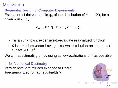
MotivationSequential Design of Computer Experiments ...Estimation of the α-quantile qα of the distribution of Y � f pXq, for agiven α in p0,1q,

qα � inf tq : PpY ¤ qq ¡ αu .� f is an unknown, expensive-to-evaluate real-valued function� X is a random vector having a known distribution on a compactsubset A � R

d .

We aim at estimating qα by using as few evaluations of f as possible

... for Numerical DosimetryAt wich level are fetuses exposed to RadioFrequency Electromagnetic Fields ?

2/16

Background: Gaussian Process ModellingAssume that f is a sample of a zero-mean Gaussian process (GP)having a covariance function k : GPp0, kp., .qqConditionally to yt � py1, . . . , yt q1, the mean µtpuq and covariancekt pu, vq are given by

µt puq � ktpuq1K�1t yt ,

kt pu, vq � kpu, vq � kt puq1K�1t ktpvq ,

where ktpuq � rkpx1,uq . . . kpxt ,uqs1, 1 denotes the matrixtransposition, Kt � rkpxi , xjqs1¤i ,j¤t , u and v and the xi ’s are in A.

Covariance functionSince the SAR is supposed to be smooth, we shall use the squareexponential covariance function

kSEpu, vq � exp��}u � v}2

2ℓ2

,u, v P A , ℓ ¡ 0 ,

where }u} denotes the euclidean norm of u in Rd .

3/16

Background: MethodologiesSequential strategiesBayesian optimization: find the maximum of f , optimizing anacquisition function� Expected Improvement [Vazquez et al., 2010]� Confidence Bound Criteria (GP-UCB [Srinivas et al., 2010],

Branch and Bounds [De Freitas et al., 2012])EI has been adapted for� Contour estimation [Ranjan et al., 2009]� Estimation of PpY ¥ sq where s is a given threshold (SUR) [Bect

et al., 2012]

Quantile estimation� Non sequential approach [Oakley, 2004]� Extension of the SUR criterion [Arnaud et al., 2010]We really need a sequential strategy, but improvement based criteriademand Monte Carlo samplings of the GP and the conditional GPs,which made them difficult to use for d ¡ 2

4/16

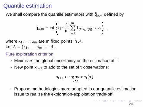
Quantile estimationWe shall compare the quantile estimators with qα,m defined by

qα,m � inf

#q :

1m

m

i�1

1tf pxi q¤qu ¡ α

+,

where x1, . . . , xm are m fixed points in A.Let A � tx1, . . . , xmu � A .

Pure exploration criterion� Minimizes the global uncertainty on the estimation of f� New point xt�1 to add to the set of t observations:

xt�1 P arg maxxPA

σt pxq .� Propose methodologies more adapted to our quantile estimationissue to realize the exploration-exploitation trade-off

5/16

GPS� Let µUt pxq � µt pxq �?

βtσt pxq and µLt pxq � µt pxq � ?

βtσt pxqwith βt � 2 ln

�π2t2

6

� 2 ln�

mδ

�where m is the cardinal of A� Let qU

α,t and qLα,t be the estimators of the α-quantile of µU

t and µLt

qUα,t � inf

#q :

1m

m

i�1

1tµUt pxi q¤qu ¡ α

+qLα,t � inf

#q :

1m

m

i�1

1tµLt pxi q¤qu ¡ α

+PropositionFor all δ in p0,1q, for all t ¥ 1, with probability greater than p1 � δq,

qα,m P rqLα,t , q

Uα,t s .

6/16

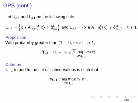
GPS (cont.)

Let Uα,t and Lα,t be the following sets :

Uα,t � !x P A : µUt pxq ¥ qL

α,t

)and Lα,t � !x P A : µL

t pxq ¤ qUα,t

), t ¥ 1.

PropositionWith probability greater than p1 � δq, for all t ¥ 1,|qα,t � qα,m| ¤aβt sup

xPUα,t

σt pxq .Criterionxt�1 to add to the set of t observations is such that:

xt�1 P arg maxxPUα,t

σt pxq .7/16

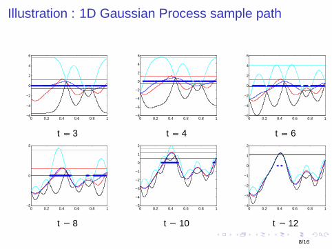
Illustration : 1D Gaussian Process sample path

0 0.2 0.4 0.6 0.8 1−6

−4

−2

0

2

4

6

0 0.2 0.4 0.6 0.8 1−8

−6

−4

−2

0

2

4

6

0 0.2 0.4 0.6 0.8 1−6

−4

−2

0

2

4

6

t � 3 t � 4 t � 6

0 0.2 0.4 0.6 0.8 1−5

0

5

0 0.2 0.4 0.6 0.8 1−5

−4

−3

−2

−1

0

1

2

0 0.2 0.4 0.6 0.8 1−4

−3

−2

−1

0

1

2

t � 8 t � 10 t � 12

8/16

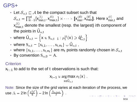
GPS+� Let Sα,t � A be the compact subset such that

Sα,t �±di�1rx piqmin,t , x

piqmax,t s � � � � � rx pdqmin, x

pdqmaxs. Here x piqmin,t and

x piqmax,t denote the smallest (resp. the largest) i th component ofthe points in Uα,t� where Uα,t � !x P Sα,t�1 : µU

t pxq ¥ qLα,t

)� where Sα,t � txt,1, . . . , xt,mt u Y Uα,t ,� where txt,1, . . . , xt,mt u are mt points randomly chosen in Sα,t� By convention Sα,0 � A.

Criterionxt�1 to add to the set of t observations is such that:

xt�1 P arg maxxPUα,t

σt pxq .Note: Since the size of the grid varies at each iteration of the process, we

use βt � 2 ln�

π2t2

6

� 2 ln� |Sα,t�1|

δ

.

9/16

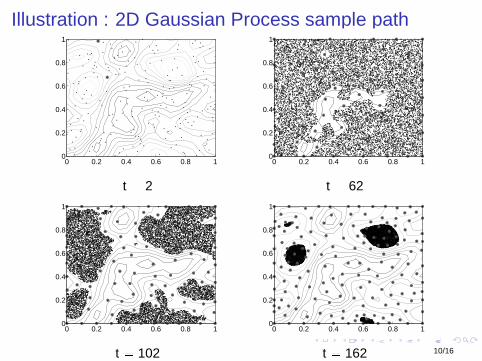
Illustration : 2D Gaussian Process sample path

0 0.2 0.4 0.6 0.8 10

0.2

0.4

0.6

0.8

1

0 0.2 0.4 0.6 0.8 10

0.2

0.4

0.6

0.8

1

t � 2 t � 62

0 0.2 0.4 0.6 0.8 10

0.2

0.4

0.6

0.8

1

0 0.2 0.4 0.6 0.8 10

0.2

0.4

0.6

0.8

1

t � 102 t � 162 10/16

Numerical Dosimetry ?In generalVirtually expose human 3D-models to one source of EMF in order toevaluate the Specific Absorption Rate (the SAR, in W .kg�1)SAR computation in our case is done through Finite Difference inTime Domain (FDTD) methodThe SAR depends on� the geometry of the models� the dielectric properties of the tissues� the type and position of the EMF source

Fetus exposure� Very few models are available� The simulations are expensive in terms of computational load� The preparation of the simulations is very complex

We focus on the fetal brain exposure

11/16

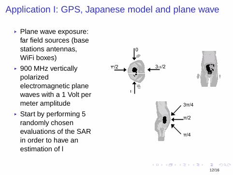
Application I: GPS, Japanese model and plane wave� Plane wave exposure:far field sources (basestations antennas,WiFi boxes)� 900 MHz verticallypolarizedelectromagnetic planewaves with a 1 Volt permeter amplitude� Start by performing 5randomly chosenevaluations of the SARin order to have anestimation of l

0

/2 3 /2

π/4

π/2

3π/4

12/16

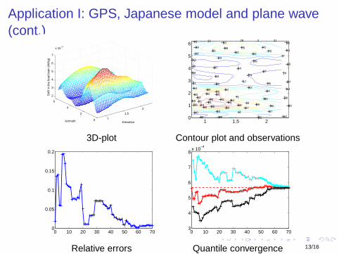
Application I: GPS, Japanese model and plane wave(cont.)

1

1.5

2

0

2

4

6

2

3

4

5

6

7

x 10−4

ElevationAzimuth

SA

R in

the

feta

l bra

in (

W/k

g)

1

2

3

4

5

6

7

8

9

10

11

12

13

14

15

16

17

18

19

20

21

2223

24

25

26

27

28

29

30

3132

33

34

35

36

37

38

39

40

41

42

43

44

45

46

47

48

49

50

51

52

53

54

55

5657

58

59

60

61

6263

64

6566

67

68

69

70

7172

73

74

75

1 1.5 20

1

2

3

4

5

6

3D-plot Contour plot and observations

0 10 20 30 40 50 60 700

0.05

0.1

0.15

0.2

0 10 20 30 40 50 60 703

4

5

6

7

8x 10

−4

Relative errors Quantile convergence 13/16

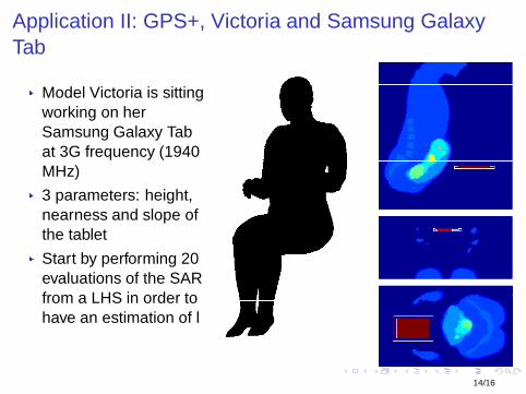
Application II: GPS+, Victoria and Samsung GalaxyTab� Model Victoria is sitting

working on herSamsung Galaxy Tabat 3G frequency (1940MHz)� 3 parameters: height,nearness and slope ofthe tablet� Start by performing 20evaluations of the SARfrom a LHS in order tohave an estimation of l

14/16

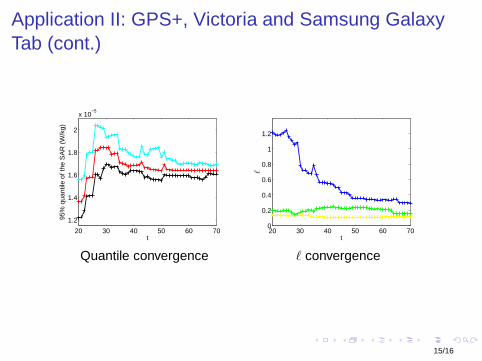
Application II: GPS+, Victoria and Samsung GalaxyTab (cont.)

20 30 40 50 60 70

1.2

1.4

1.6

1.8

2

x 10−5

t

95%

qua

ntile

of t

he S

AR

(W

/kg)

20 30 40 50 60 700

0.2

0.4

0.6

0.8

1

1.2

t

ℓQuantile convergence ℓ convergence

15/16

Conclusion

� We propose two novel sequential approaches for quantileestimation� Successfully applied to real data coming from numericaldosimetry

16/16