EE363 Winter 2008-09

Review Session 5

• a partial summary of the course

• no guarantees everything on the exam is covered here

• not designed to stand alone; use with the class notes

5–1

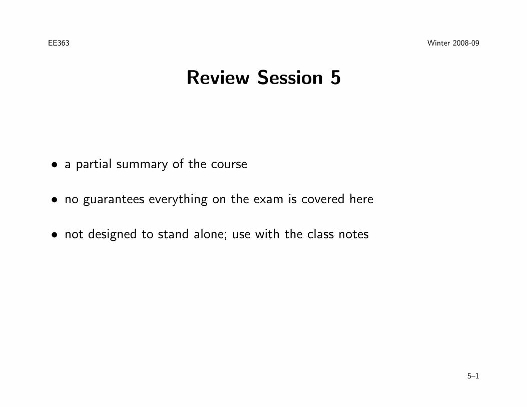
LQR

• balance good control and small input effort

• quadratic cost function

J(U) =N−1∑

τ=0

(

xTτ Qxτ + uT

τ Ruτ

)

+ xTNQfxN

• Q, Qf and R are state cost, final state cost, input cost matrices

5–2

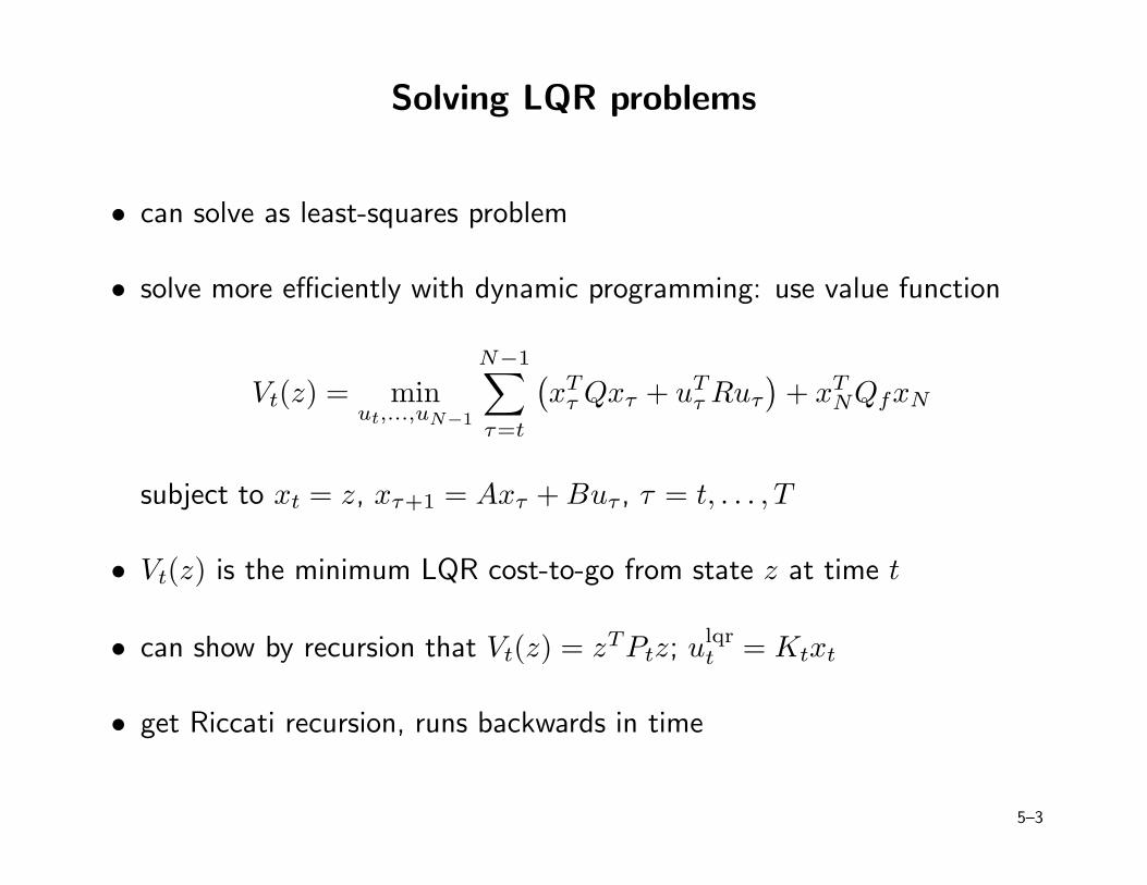
Solving LQR problems

• can solve as least-squares problem

• solve more efficiently with dynamic programming: use value function

Vt(z) = minut,...,uN−1

N−1∑

τ=t

(

xTτ Qxτ + uT

τ Ruτ

)

+ xTNQfxN

subject to xt = z, xτ+1 = Axτ + Buτ , τ = t, . . . , T

• Vt(z) is the minimum LQR cost-to-go from state z at time t

• can show by recursion that Vt(z) = zTPtz; ulqrt = Ktxt

• get Riccati recursion, runs backwards in time

5–3

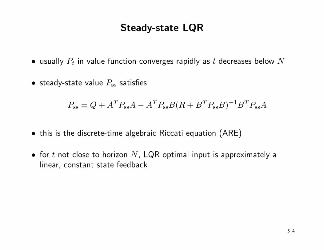
Steady-state LQR

• usually Pt in value function converges rapidly as t decreases below N

• steady-state value Pss satisfies

Pss = Q + ATPssA − ATPssB(R + BTPssB)−1BTPssA

• this is the discrete-time algebraic Riccati equation (ARE)

• for t not close to horizon N , LQR optimal input is approximately alinear, constant state feedback

5–4

LQR extensions

• time-varying systems

• time-varying cost matrices

• tracking problems (with state/input offsets)

• Gauss-Newton LQR for nonlinear dynamical systems

• can view LQR as solution of constrained minimization problem, viaLagrange multipliers

5–5

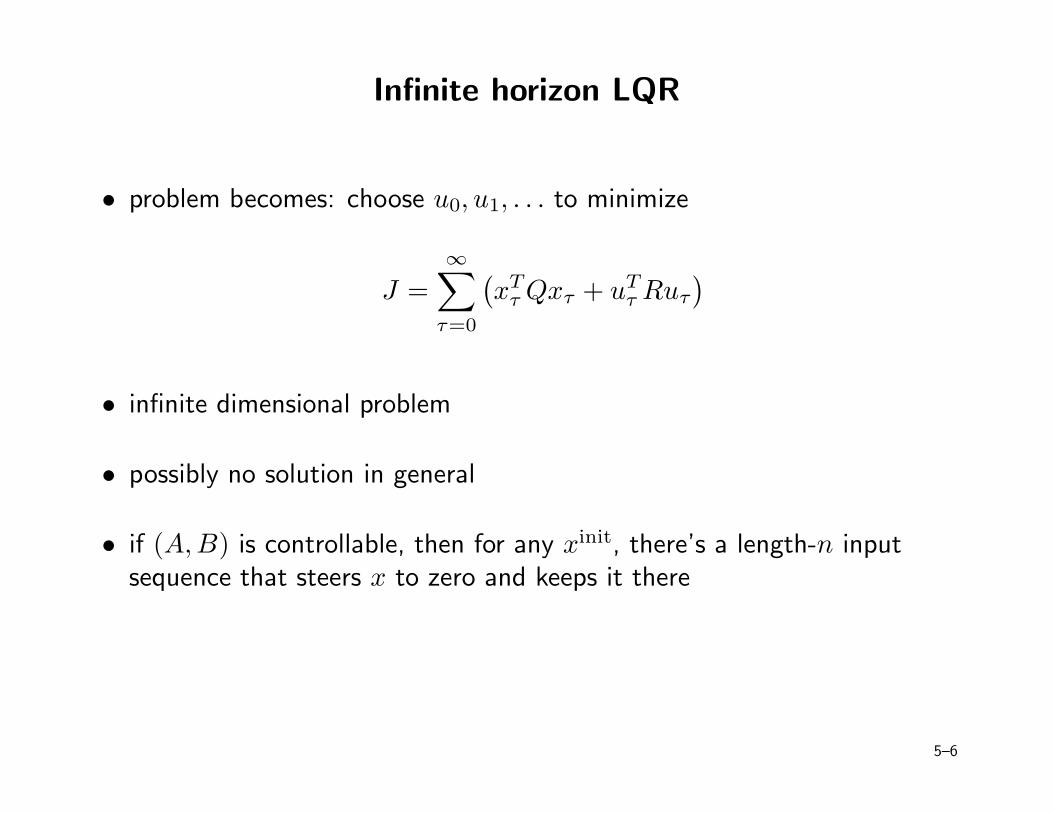
Infinite horizon LQR

• problem becomes: choose u0, u1, . . . to minimize

J =

∞∑

τ=0

(

xTτ Qxτ + uT

τ Ruτ

)

• infinite dimensional problem

• possibly no solution in general

• if (A,B) is controllable, then for any xinit, there’s a length-n inputsequence that steers x to zero and keeps it there

5–6

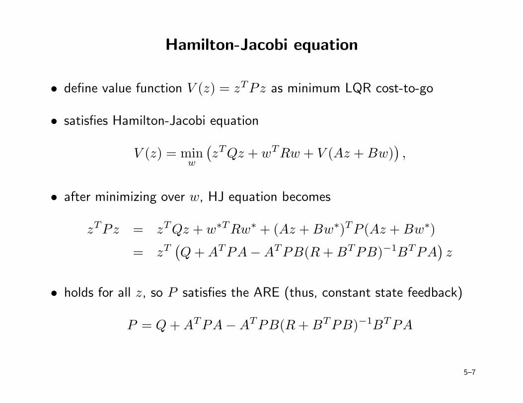
Hamilton-Jacobi equation

• define value function V (z) = zTPz as minimum LQR cost-to-go

• satisfies Hamilton-Jacobi equation

V (z) = minw

(

zTQz + wTRw + V (Az + Bw))

,

• after minimizing over w, HJ equation becomes

zTPz = zTQz + w∗TRw∗ + (Az + Bw∗)TP (Az + Bw∗)

= zT(

Q + ATPA − ATPB(R + BTPB)−1BTPA)

z

• holds for all z, so P satisfies the ARE (thus, constant state feedback)

P = Q + ATPA − ATPB(R + BTPB)−1BTPA

5–7

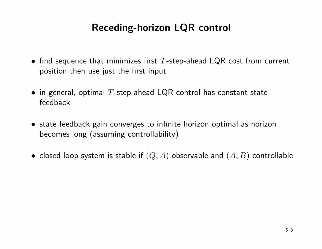
Receding-horizon LQR control

• find sequence that minimizes first T -step-ahead LQR cost from currentposition then use just the first input

• in general, optimal T -step-ahead LQR control has constant statefeedback

• state feedback gain converges to infinite horizon optimal as horizonbecomes long (assuming controllability)

• closed loop system is stable if (Q,A) observable and (A, B) controllable

5–8

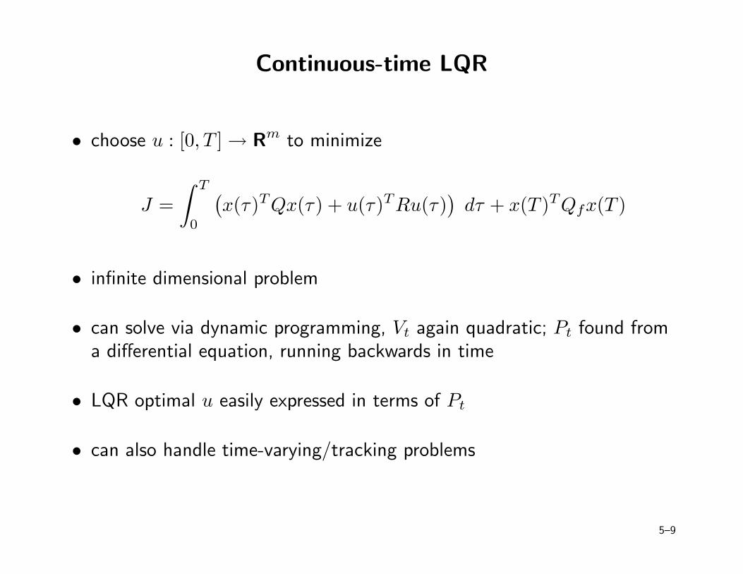
Continuous-time LQR

• choose u : [0, T ] → Rm to minimize

J =

∫ T

0

(

x(τ)TQx(τ) + u(τ)TRu(τ))

dτ + x(T )TQfx(T )

• infinite dimensional problem

• can solve via dynamic programming, Vt again quadratic; Pt found froma differential equation, running backwards in time

• LQR optimal u easily expressed in terms of Pt

• can also handle time-varying/tracking problems

5–9

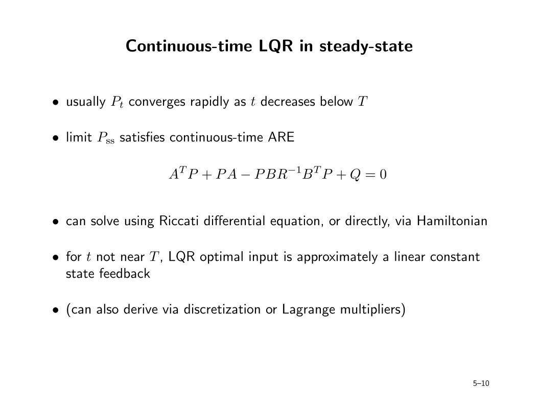
Continuous-time LQR in steady-state

• usually Pt converges rapidly as t decreases below T

• limit Pss satisfies continuous-time ARE

ATP + PA − PBR−1BTP + Q = 0

• can solve using Riccati differential equation, or directly, via Hamiltonian

• for t not near T , LQR optimal input is approximately a linear constantstate feedback

• (can also derive via discretization or Lagrange multipliers)

5–10

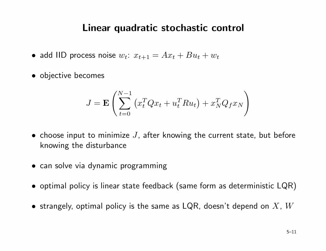
Linear quadratic stochastic control

• add IID process noise wt: xt+1 = Axt + But + wt

• objective becomes

J = E

(

N−1∑

t=0

(

xTt Qxt + uT

t Rut

)

+ xTNQfxN

)

• choose input to minimize J , after knowing the current state, but beforeknowing the disturbance

• can solve via dynamic programming

• optimal policy is linear state feedback (same form as deterministic LQR)

• strangely, optimal policy is the same as LQR, doesn’t depend on X , W

5–11

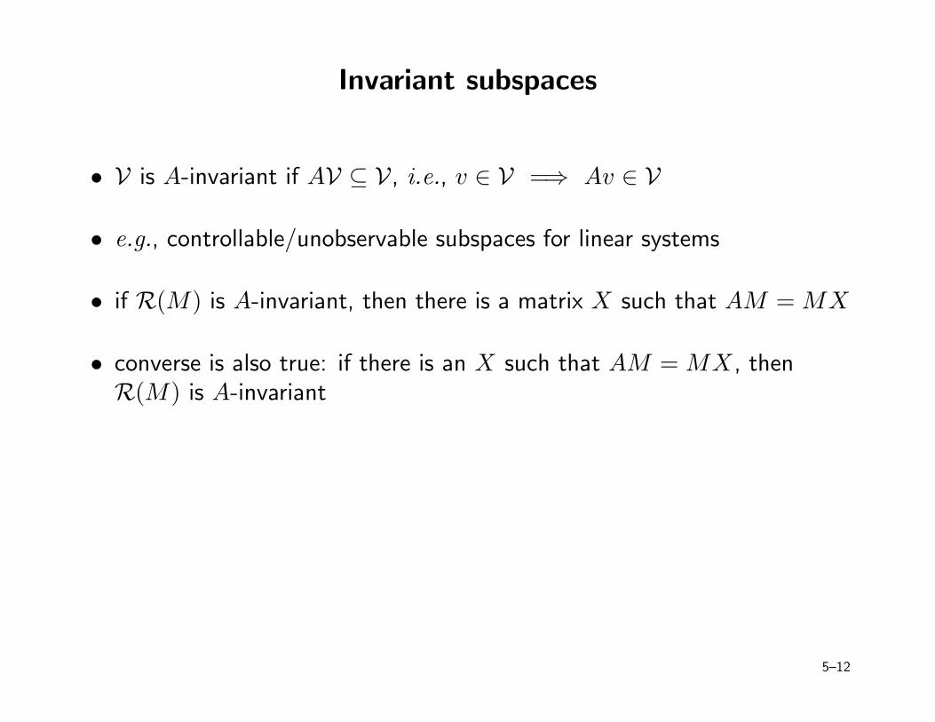
Invariant subspaces

• V is A-invariant if AV ⊆ V , i.e., v ∈ V =⇒ Av ∈ V

• e.g., controllable/unobservable subspaces for linear systems

• if R(M) is A-invariant, then there is a matrix X such that AM = MX

• converse is also true: if there is an X such that AM = MX , thenR(M) is A-invariant

5–12

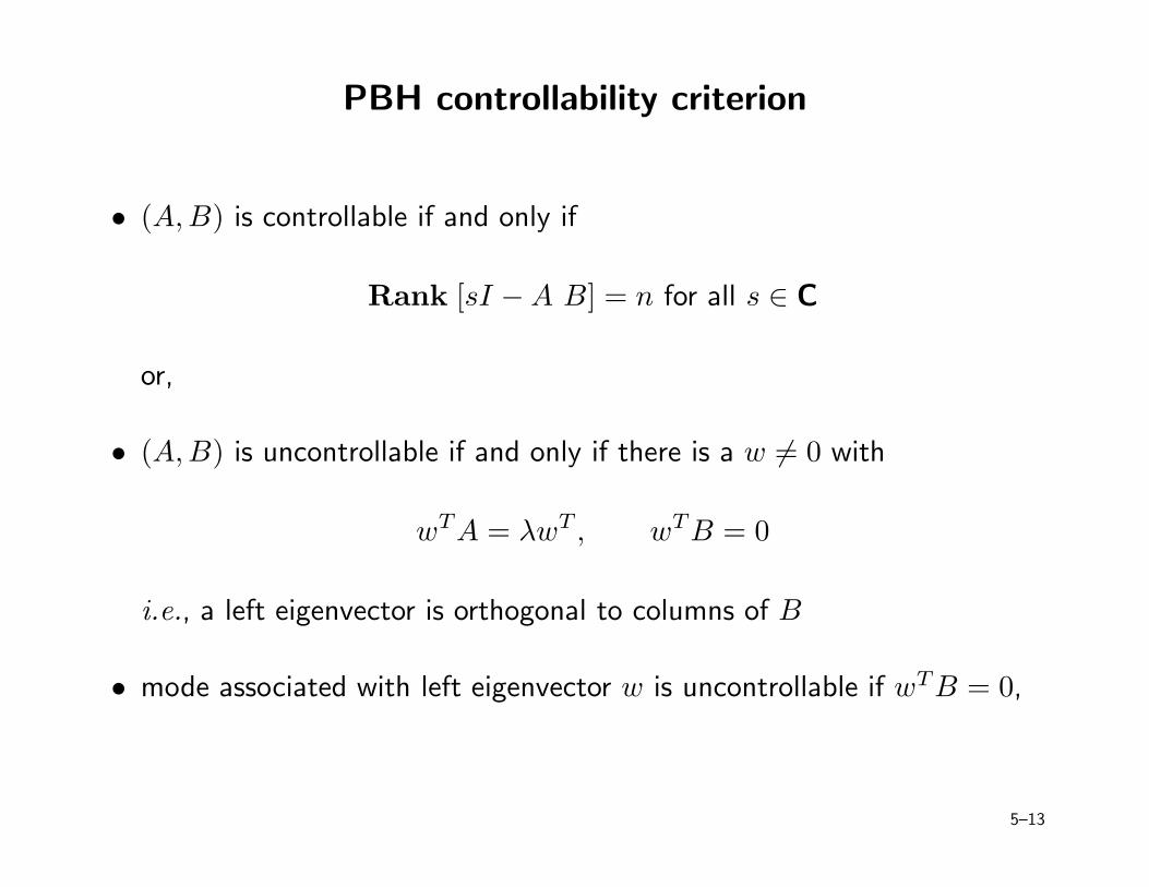
PBH controllability criterion

• (A,B) is controllable if and only if

Rank [sI − A B] = n for all s ∈ C

or,

• (A,B) is uncontrollable if and only if there is a w 6= 0 with

wTA = λwT , wTB = 0

i.e., a left eigenvector is orthogonal to columns of B

• mode associated with left eigenvector w is uncontrollable if wTB = 0,

5–13

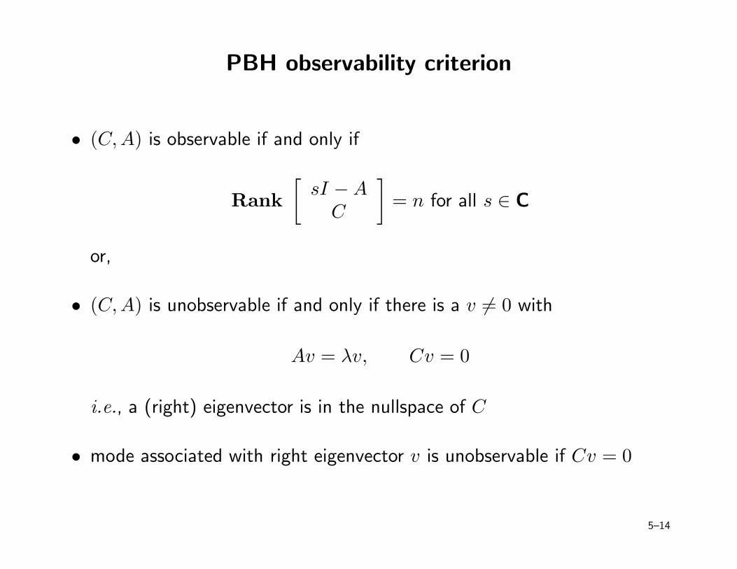
PBH observability criterion

• (C,A) is observable if and only if

Rank

[

sI − A

C

]

= n for all s ∈ C

or,

• (C,A) is unobservable if and only if there is a v 6= 0 with

Av = λv, Cv = 0

i.e., a (right) eigenvector is in the nullspace of C

• mode associated with right eigenvector v is unobservable if Cv = 0

5–14

Estimation

• minimum mean-square estimator (MMSE) is, in general, E(x|y)

• for jointly Gaussian x and y, MMSE estimator of x is affine function of y

x = φmmse(y) = x + ΣxyΣ−1y (y − y)

• when x, y aren’t jointly Gaussian, best linear unbiased estimator is

x = φblu(y) = x + ΣxyΣ−1y (y − y)

• φblu is unbiased (E x = Ex), often works well, has MMSE among allaffine estimators

• given A, Σx, Σv, can evaluate Σest before knowing measurements(can do experiment design)

5–15

Linear system with stochastic process

• covariance Σx(t) satisfies a Lyapunov-like linear dynamical system

Σx(t + 1) = AΣx(t)AT + BΣu(t)BT + AΣxu(t)BT + BΣux(t)AT

• if Σxu(t) = 0 (x and u uncorrelated), we have the Lyapunov iteration

Σx(t + 1) = AΣx(t)AT + BΣu(t)BT

• if (and only if) A is stable, converges to steady-state covariance whichsatisfies the Lyapunov equation

Σx = AΣxAT + BΣuBT

5–16

Kalman filter

• estimate current or next state, based on current and past outputs

• recursive, so computationally efficient (can express as Riccati recursion)

• measurement update

xt|t = xt|t−1 + Σt|t−1CT(

CΣt|t−1CT + V

)−1(yt − Cxt|t−1)

Σt|t = Σt|t−1 − Σt|t−1CT(

CΣt|t−1CT + V

)−1CΣt|t−1

• time update

xt+1|t = Axt|t, Σt+1|t = AΣt|tAT + W

• can compute Σt|t−1 before any observations are made

• steady-state error covariance satisfies AREΣ = AΣAT + W − AΣCT (CΣCT + V )−1CΣAT

5–17

Approximate nonlinear filtering

• in general, exact solution is impractical; requires propagating infinitedimensional conditional densities

• extended Kalman filter: use affine approximations of nonlinearities,Gaussian model

• other methods (e.g., particle filters): based on Monte Carlo methodsthat sample the random variables

• usually heuristic, unless problems are very small

5–18

Conservation and dissipation

• a set C ⊆ Rn is invariant with respect to autonomous, time-invariant,nonlinear x = f(x) if for every trajectory x,

x(t) ∈ C =⇒ x(τ) ∈ C for all τ ≥ t

• every trajectory that enters or starts in C must stay there

• scalar valued function φ is a conserved quantity for x = f(x) if for everytrajectory x, φ(x(t)) is constant

• φ is a dissipated quantity for x = f(x) if for every trajectory x, φ(x(t))is (weakly) decreasing

5–19

Quadratic functions and linear dynamical systems

continuous time: linear system x = Ax, quadratic form φ(z) = zTPz

• φ is conserved if and only if ATP + PA = 0

• φ is dissipated if and only if ATP + PA ≤ 0

discrete time: linear system xt+1 = Axt, quadratic form φ(z) = zTPz

• φ is conserved if and only if ATPA − P = 0

• φ is dissipated if and only if ATPA − P ≤ 0

5–20

Stability

consider nonlinear time-invariant system x = f(x)

• xe is an equilibrium point if f(xe) = 0

• system is globally asymptotically stable (GAS) if for every trajectory x,x(t) → xe as t → ∞

• system is locally asymptotically stable (LAS) near or at xe, if there is anR > 0 such that ‖x(0) − xe‖ ≤ R =⇒ x(t) → xe as t → ∞

• for linear systems (with xe = 0), LAS ⇔ GAS ⇔ ℜλi(A) < 0

5–21

Energy and dissipation functions

consider nonlinear time-invariant system x = f(x), function V : Rn → R

• define V : Rn → R as V (z) = ∇V (z)Tf(z)

• V (z) givesd

dtV (x(t)) when z = x(t), x = f(x)

• can think of V as generalized energy function, −V as the associatedgeneralized dissipation function

• V is positive definite if V (z) ≥ 0 for all z, V (z) = 0 if and only if z = 0and all sublevel sets of V are bounded (V (z) → ∞ as z → ∞)

5–22

Lyapunov theory

• used to make conclusions about of system trajectories, without findingthe trajectories

• boundedness: if there is a (Lyapunov function) V with all sublevel setsbounded, and V (z) ≤ 0 for all z, then all trajectories are bounded

• global asymptotic stability: if there is a positive definite V withV (z) < 0 for all z 6= 0 and V (0) = 0, then every trajectory of x = f(x)converges to zero as t → ∞

• exponential stability: if there is a positive definite V , and constantα > 0 with V (z) ≤ −αV (z) for all z, then there is an M such thatevery trajectory satisfies ‖x(t)‖ ≤ Me−αt/2‖x(0)‖

5–23

Lasalle’s theorem

• can conclude GAS of a system with only V ≤ 0 and anobservability-type condition

• if there is a positive definite V with V (z) ≤ 0, and the only solution ofw = f(w), V (w) = 0 is w(t) = 0 for all t, then the system is GAS

• requires time-invariance

5–24

Converse Lyapunov theorems

• if a linear system is GAS, there is a quadratic Lyapunov function thatproves it

• if a system is globally exponentially stable, there is a Lyapunov functionthat proves it

5–25

Linear quadratic Lyapunov theory

• Lyapunov equation: ATP + PA + Q = 0

• for linear system x = Ax, if V (z) = zTPz, thenV (z) = (Az)TPz + zTP (Az) = −zTQz

• if zTPz is the generalized energy, then zTQz is the associatedgeneralized dissipation

• boundedness: if P > 0, Q ≥ 0, then all trajectories are bounded, andthe ellipsoids {z | zTPz ≤ a} are invariant

• stability: if P > 0, Q > 0, then the system is GAS

• an extension from Lasalle’s theorem: if P > 0, Q ≥ 0 and (Q,A)observable, then the system is GAS

• if Q ≥ 0 and P 6≥ 0, then A is not stable

5–26

The Lyapunov operator

• the Lyapunov operator is given by

L(P ) = ATP + PA

• if A is stable, Lyapunov operator is nonsingular

• if A has imaginary eigenvalue, then Lyapunov operator is singular

• thus, if A is stable, for any Q there is exactly one solution P of theLyapunov equation ATP + PA + Q = 0

• efficient ways to solve the Lyapunov equation (review session 3)

5–27

The Lyapunov integral

• if A is stable, explicit formula for solution of Lyapunov equation:

P =

∫ ∞

0

etATQetA dt

• if A is stable, P is unique solution of Lyapunov equation, then

V (z) = zTPz =

∫ ∞

0

x(t)TQx(t) dt

(where x = Ax and x(0) = z)

• thus, V (z) is cost-to-go from point z, and integral quadratic costfunction with matrix Q

• can use to evaluate quadratic integrals

5–28

Further Lyapunov results

• all linear quadratic Lyapunov results have discrete-time counterparts

• discrete-time Lyapunov equation is

ATPA − P + Q = 0

(if V (z) = zTPz, then δV (z) = −zTQz)

• for a nonlinear system x = f(x) with xe an equilibrium point, if thelinearized system near xe is stable, then the nonlinear system is locallyasymptotically stable (and nearly vice versa)

5–29

LMIs

• the Lyapunov inequality ATP + PA + Q ≤ 0 is an LMI in variable P

• P satisfies the Lyapunov LMI if and only if the quadratic formV (z) = zTPz satisfies V (z) ≤ −zTQz

• bounded-real LMI: if P satisfies

[

ATP + PA + CTC PB

BTP −γ2I

]

≤ 0, P ≥ 0

then the quadratic Lyapunov function V (z) = zTPz proves the RMSgain of the system is no more than γ

5–30

Using LMIs

• practical approach to strict matrix inequalities: if inequalities arehomogeneous in x, replace Fstrict(x) > 0 with Fstrict(x) ≥ I

• if inequalities aren’t homogeneous, replace Fstrict(x) > 0 withFstrict(x) ≥ ǫI, with ǫ small and positive

• if we have x(t) = A(t)x(t), with A(t) ∈ {A1, . . . , AK}, can usemultiple simultaneous LMIs to find a simultaneous Lyapunov functionthat establishes a property for all trajectories

• can’t be done analytically, but possible to do numerically

• more generally, can globally and efficiently solve SDPs:

minimize cTx

subject to F0 + x1F1 + · · · + xnFn ≥ 0Ax = b

5–31

S-procedure

• for two quadratic forms, if and (with a constraint qualification) only ifthere is a τ ≥ 0 with F0 ≥ τF1, then zTF1z ≥ 0 =⇒ zTF0z ≥ 0

• can also replace ≥ with >

• for multiple quadratic forms, if there are τ1, . . . , τk ≥ 0 with

F0 ≥ τ1F1 + · · · + τkFk

then, for all z,

zTF1z ≥ 0, . . . , zTFkz ≥ 0 ⇒ zTF0z ≥ 0

• can solve using LMIs

5–32

Systems with sector nonlinearities

• a function φ : R → R is said to be in sector [l, u] if for all q ∈ R,p = φ(q) lies between lq and uq

• a (single nonlinearity) Lur’e system has the form

x = Ax + Bp, q = Cx, p = φ(t, q)

where φ(t, ·) : R → R is in sector [l, u] for each t

• goal: prove stability or bound using only the sector information

5–33

GAS of Lur’e system

• can express GAS of Lur’e system using quadratic Lyapunov functionV (z) = zTPz as requiring V + αV ≤ 0, equivalent to

[

z

p

]T [ATP + PA + αP PB

BTP 0

] [

z

p

]

≤ 0

whenever[

z

p

]T [σCTC −νCT

−νC 1

] [

z

p

]

≤ 0

• can convert this to the LMI (with variables P and τ)

[

ATP + PA + αP − τσCTC PB + τνCT

BTP + τνC −τ

]

≤ 0, P ≥ I

• can sometimes extend to case with multiple nonlinearities

5–34

Perron-Frobenius theory

• a nonegative matrix A is regular if for some k ≥ 1, Ak > 0(path of length k from every node to every other node)

• if A is regular, then there is a real, positive, strictly dominant, simplePerron-Frobenius eigenvalue λpf , with positive left and righteigenvectors

• if we only have A ≥ 0, then there is an eigenvalue λpf of A that is real,nonnegative and (non-strictly) dominant, and has (possibly not unique)nonnegative left and right eigenvectors

• For a Markov chain with transition matrix P , if P is regular, thedistribution always converges to the unique invariant distribution π > 0,associated with a simple, dominant eigenvalue of 1

• rate of convergence depends on second largest eigenvalue magnitude

5–35

Max-min/min-max ratio characterization

• Perron-Frobenius eigenvalue is optimal value of two optimizationproblems

maximize mini(Ax)i

xi

subject to x > 0

andminimize maxi

(Ax)ixi

subject to x > 0

• the optimal x is the Perron-Frobenius eigenvector

5–36

Linear Lyapunov functions

• suppose c > 0, and consider the linear Lyapunov function V (z) = cTz

• if V (Az) ≤ δV (z) for some δ < 1 and all z ≥ 0, then V proves(nonnegative) trajectories converge to zero

• a nonnegative regular system is stable if and only if there is a linearLyapunov function that proves it

5–37

Continuous time results

• Rn+ is invariant under x = Ax if and only if Aij ≥ 0 for i 6= j

• such matrices are called Metzler matrices

• A has a real, dominant eigenvalue λmetzler that is real and hasassociated nonnegative left and right eigenvectors

• analogs exist with other discrete-time results

5–38

Exam advice

• five questions

• determine the topic(s) each question covers

• guess the form the problem statement should take

• manipulate (‘hammer’) the question into that standard form

• explain things as simply as possible; if your solution is extremelycomplicated, you’re probably missing something

• we’re not especially concerned about boundary conditions or edge cases,but mention any assumptions you make

5–39