QUENCHED AND ANNEALED TEMPORAL LIMITTHEOREMS FOR CIRCLE ROTATIONS.

DMITRY DOLGOPYAT AND OMRI SARIG

In memory of Jean-Christophe Yoccoz

Abstract. Let h(x) = x − 12 . We study the distribution of∑n−1

k=0 h(x+ kα) when x is fixed, and n is sampled randomly uni-formly in 1, . . . , N, as N → ∞. Beck proved in [Bec10, Bec11]that if x = 0 and α is a quadratic irrational, then these distribu-tions converge, after proper scaling, to the Gaussian distribution.We show that the set of α where a distributional scaling limit ex-ists has Lebesgue measure zero, but that the following annealedlimit theorem holds: Let (α, n) be chosen randomly uniformly in

R/Z× 1, . . . , N, then the distribution of∑n−1

k=0 h(kα) convergesafter proper scaling as N →∞ to the Cauchy distribution.

1. Introduction

We study the centered ergodic sums of functions h : T → R for therotation by a an irrational angle α

(1.1) Sn(α, x) =

(n∑k=1

h(x+ kα)

)− n

∫Th(z)dz.

Weyl’s equidistribution theorem says that for every α ∈ R \Q, and forevery h Riemann integrable, 1

nSn(α, x) −−−→

n→∞0 uniformly in x. We are

interested in higher-order asymptotics. We aim at results which holdfor a set of full Lebesgue measure of α.

If h is sufficiently smooth, then Sn(α, x) is bounded for almost everyα and all x (see [Her79] or appendix A). The situation for piecewisesmooth h is more complicated, and not completely undertstood evenfor functions with a single singularity.

2010 Mathematics Subject Classification. 37D25 (primary), 37D35 (secondary).D. D. acknowledges the support of the NSF grant DMS1665046. O.S. acknowl-

edges the support of the ISF grant 199/14.1

2 DMITRY DOLGOPYAT AND OMRI SARIG

Setup. Here we study (1.1), for the simplest example of a piecewisesmooth function with one discontinuity on T = R/Z:

(1.2) h(x) = x − 1

2.

The fractional part x is the unique t ∈ [0, 1) s.t. x ∈ t+ Z.Case (1.2) is sufficient for understanding the behavior for typical α

for all functions f(t) on T which are differentiable everywhere exceptone point x0, and whose derivative on T\x0 extends to a function ofbounded variation on T. This is because of the following result provenin Appendix A:

Proposition 1.1. If f(t) is differentiable on T \ x1, . . . , xν and f ′

extends to a function with bounded variation on T, then there areA1, . . . , Aν ∈ R s.t. for a.e. α there is ϕα ∈ C(T) s.t. for all x 6= xi,

f(x) =ν∑i=1

Aih(x+ xi) +

∫Tf(t)dt+ ϕα(x)− ϕα(x+ α).

Of course there are many functions h for which Proposition 1.1 holds.The choice (1.2) is convenient, because of its nice Fourier series.

Methodology. Sn(α, x) is very oscillatory. Therefore, instead of look-ing for simple asymptotic formulas for Sn(α, x), which is hopeless, wewill look for simple scaling limits for the distribution of Sn(α, x) whenx, or α, or n (or some of their combinations) are randomized. Thereare several natural ways to carry out the randomization:

(1) Spatial vs temporal limit theorems: In a spatial limit theorem, theinitial condition x chosen randomly from the space T. In a temporallimit theorem, the initial condition x is fixed, and the “time” n ischosen randomly uniformly in 1, . . . , N as N →∞. Neither limittheorem implies the other, see [DS17].

(2) Quenched vs annealed limit theorems: In a quenched limit theorem,α is fixed. In an annealed limit theorem α is randomized. Theterminology is motivated by the theory of random walks in randomenvironment; the parameter α is the “environment parameter.”

We indicate what is known and what is still open in our case.

Known results on spatial limit theorems: The quenched spatiallimit theorem fails; the annealed spatial limit theorem holds.

The failure of the quenched spatial limit theorem is very general.Namely, It follows from the Denjoy-Koksma inequality that there areno quenched spatial distributional limit theorems for any rotation byα ∈ R \ Q, and every function of bounded variation which is not a

QUENCHED AND ANNEALED TLTS FOR CIRCLE ROTATIONS. 3

coboundary (e.g. h(x) = x− 12). In the coboundary case, the spatial

limit theorem is trivial. Many people have looked for weaker quenchedversions of spatial distributional limit theorem (e.g. along special sub-sequences of “times”). See [DF15, DS17] for references and furtherdiscussion.

The annealed spatial limit theorem is a famous result of Kesten.

Theorem 1.2. ([Kes60]) If (x, α) is uniformly distributed on T × Tthen the distribution of Sn(α,x)

lnnconverges as n → ∞ to a symmetric

Cauchy distribution: ∃ρ1 6= 0 s.t. for all t ∈ R,

limn→∞

P(Sn(α, x)

lnn≤ t

)=

1

2+

arctan(t/ρ1)

π.

See [Kes60] for the value of constant ρ1. The same result holds forh(x) = 1[0,β)(x) − β with β ∈ R, with different ρ1 = ρ1(β) [Kes60,Kes62].

Known results on temporal limit theorems: Quenched temporallimit theorems are known for special α; There were no results on theannealed temporal limit theorem until this work.

The first temporal limit theorem for an irrational rotation (indeedfor any dynamical system) is due to J. Beck [Bec10, Bec11]. Let

MN(α, x) :=1

N

N∑n=1

Sn(α, x) , Sn(α, x) := Sn(α, x)−MN(α, x).

Theorem 1.3 (Beck). Let α be an irrational root of a quadratic polyno-mial with integer coefficients. Fix x = 0. If n is uniformly distributed

on 1 . . . N then Sn(α,x)√lnN

converges to a normal distribution as N →∞.

A similar result holds for the same x and α with h(x) = x − 12

replaced by 1[0,β)(x) − β, β ∈ Q [Bec10, Bec11]. [ADDS15, DS17]extended this to all x ∈ [0, 1). A remarkable recent paper by Bromberg& Ulcigrai [BU] gives a further extension to all x, all irrational α ofbounded type, and for an uncountable collection of β (which depends onα). Recall that the set of α of bounded type is a set of full Hausdorffdimension [Jar29], but zero Lebesgue measure [Khi24].

This paper: We show that for h(x) = x− 12, the quenched temporal

limit theorem fails for a.e. α, but that the annealed temporal limittheorem holds. See §2 for precise statements.

4 DMITRY DOLGOPYAT AND OMRI SARIG

Heuristic overview of the proof. When we expand the ergodicsums of h into Fourier series, we find that the resulting trigonomet-ric series can be split into the contribution of “resonant” and “non-resonant” harmonics.

The non-resonant harmonics are many in number, but small in size.They tend to cancel out, and their total contribution is of order

√lnN .

It is natural to expect that this contribution has Gaussian statistics. Ifα has bounded type, all harmonics are non-resonant, and as Brombergand Ulcigrai show in the case 1[0,β) − β the limiting distribution isindeed Gaussian.

The resonant harmonics are small in number, but much larger in size:Individual resonant harmonics have contribution of order lnN . Fortypical α, the number, strength, and location of the resonant harmonicschanges erratically with N in a non-universal way. This leads to thefailure of temporal distributional limit theorems for typical α.

We remark that a similar obstruction to quenched limit theoremshave been observed before in the theory of random walks in randomenvironment [DG12, PS13, CGZ00].

To justify this heuristic we fix N and compute the distribution ofresonances when α is uniformly distributed. Since the distribution ofresonances is non-trivial, changing a scale typically leads to a differenttemporal distribution proving that there is no limit as N → ∞. Asa byproduct of our analysis we obtain some insight on the frequencywith which a given limit distribution occurs.

Functions with more than one discontinuity. In a separate paperwe use a different method to show that given a piecewise smooth dis-continuous function with arbitrary finite number of discontinuities, thequenched temporal limit theorems fails for Lebesgue almost all α. Butthis method does not provide an annealed result, and it does not giveus as detailed information as we get here on the scaling limits whichappear along subsequences for typical α.

2. Statement of results

Fix x ∈ T arbitrary. Let Sn(α, x) :=∑n

k=1 h(x+ kα), and

MN(α, x) =1

N

N∑n=1

Sn(α, x),

Sn(α, x) = Sn(α, x)−MN(α, x).

QUENCHED AND ANNEALED TLTS FOR CIRCLE ROTATIONS. 5

Consider the cumulative distribution function of Sn(α,x)lnN

:

FN(α)(z) = FxN(α)(z) =1

NCard

(1 ≤ n ≤ N :

Sn(α, x)

lnN≤ z

).

When α is random FN(α) becomes a random element in the space Xof distribution functions endowed with Prokhorov topology.

We begin with the annealed temporal distributional limit theorem:

Theorem 2.1. Fix x ∈ T arbitrary. Let (α, n) be uniformly distributed

on T × 1, . . . , N. Then Sn(α,x)lnN

converges in law as N → ∞ to the

symmetric Cauchy distribution with scale parameter 13π√

3:

(2.1) limN→∞

P(Sn(α, x)

lnN≤ t

)=

1

2+

arctan(t/ρ2)

π(t ∈ R)

(2.2) ρ2 =1

3π√

3.

Next we turn to the quenched result, beginning with some prepa-rations. Recall (see e.g. [DF, Section 2.1]) that the Cauchy randomvariable can be represented up to scaling as

(2.3) C =∞∑m=1

Θm

ξm

where Ξ = ξm is a Poisson process on R and Θm are i.i.d boundedrandom variables with zero mean independent of Ξ. To make our ex-position more self-contained we recall the derivation of (2.3) in Appen-dix B.

In our case Θm will be distributed like the following random variableΘ. Let θ be uniformly distributed on [0, 1] and define

(2.4) Θ(θ) =∞∑k=1

cos(2πkθ)

2π2k2, θ ∼ U [0, 1].

Notice that

(2.5) Θ(θ) =θ2 − θ

2+

1

12on [0, 1],

as can be verified by expanding θ2−θ2

+ 112

on [0, 1] into a Fourier series.

Notice also that for every θ ∈ [0, 1], Θ(θ) = ζ2

2− 1

24, where ζ = θ − 1

2.

6 DMITRY DOLGOPYAT AND OMRI SARIG

Thus − 124≤ Θ ≤ 1

12, and

(2.6) P(Θ < t) =

0 t ≤ − 1

24

2√

2t+ 112

t ∈ (− 124, 1

12)

1 t > 112.

Next, given a sequence Ξ = ξm s.t.∑

m ξ−2m <∞ we can define

(2.7) CΞ =∑m

Θm

ξm

where Θm are i.i.d. random variables with distribution given by (2.6).(In the proof of Theorem 2.1, ξm would describe the small denomina-tors of Sn and Θm would describe the corresponding numerators, seeformula (3.2) in Section 3.) The sum in (2.7) converges almost surelydue to Kolmogorov’s Three Series Theorem (note that (2.4) easily im-plies that E(Θ) = 0). Let FΞ be the cumulative distribution functionof CΞ. If Ξ is a Poisson process on R, then FΞ is a random element ofProkhorov’s space X.

Theorem 2.2. Fix x ∈ T arbitrary. If α has absolutely continuousdistribution on T with bounded density then FN(α) converges in law asN →∞ to FΞ where Ξ is the Poisson process on R with intensity

(2.8) c =6

π2.

A similar result has been proven for sub-diffusive random walks inrandom environment in [DG12] with the following distinctions:

(1) for random walks Θm+1 have exponential distribution rather thanthe distribution given by (2.4)

(2) For random walk the Poisson process in the denominator of (2.3)is supported on R+ and can have intensity cx−s with s 6= 0.

We now explain how to use Theorem 2.2 to show that for a.e. α, thereis no non-trivial temporal distributional limit theorem for Sn(α, x). Itis enough to show that for a.e. α, one can find several sequences Nk

with different scaling limits for Sn(α, x) as n ∼ U1, . . . , Nk. Let

D(Θ) := finite linear combinations of i.i.d. with distribution Θ(closure in X).

Corollary 2.3. Fix x ∈ T arbitrary. For a.e. α, for every Y ∈ D(Θ),there are Nk →∞, Bk →∞, Ak ∈ R s.t.

(2.9)Sn(α, x)− Ak

Bk

dist−−−→k→∞

Y, as n ∼ U1, . . . , Nk.

QUENCHED AND ANNEALED TLTS FOR CIRCLE ROTATIONS. 7

In particular, for a.e. α, the distribution of Θ (2.6), and the normaldistribution are distributional limit points of properly rescaled ergodicsums Sn(α, x) as n ∼ U1, . . . , N.

Proof. Put on X the probability measure µ induced by the FΞ, when Ξis the Poisson point process with intensity c as in Theorem 2.2.

Observe that for every Y ∈ D(Θ),

(2.10) ∃ decreasing seq. of open Un ⊂ X s.t. µ(Un) > 0 and Un ↓ Y .

Indeed, fix a countable dense set fnn≥1 ⊂ Cc(R), and let Un :=⋂ni=1X : |EX(fi) − EY (fi)| < 1

n, then Un ↓ Y . Since Y ∈ D(Θ),

∃a1 < · · · < ak and iid Θi ∼ Θ s.t. X :=∑k

i=1 aiΘi ∈ Un. Sincef1, . . . , fn are uniformly continuous with compact support, there isδ > 0 s.t. if X1, X2 are random variables s.t. there is a couplingwith P(|X1 − X2| ≥ δ) ≤ δ then for each i ∈ 1, . . . n we have

|EX1(fi)− EX2(fi)| <1

n. Note that given a sequence bi ∈ `2

E

(∑i

biΘi

)= 0, Var

(∑i

biΘi

)= Var(Θ)

∑i

b2i .

Accordingly, the Chebyshev inequality shows that if Ξ = ξi is asequence s.t.

(2.11)k∑i=1

∣∣∣∣ 1

ai− 1

ξi

∣∣∣∣2 +∞∑

i=k+1

1

ξ2i

≤ δ2

Var(Θ)

then FΞ ∈ Un. It remains to note that if Ξ = ξi is a Poisson pointprocess then for each δ > 0, (2.11) holds with positive probability.Indeed let Aδ,R be the event that of Ξ∩ [−R,R] consists of there being

exactly k points ξ1, . . . , ξk andk∑i=1

∣∣∣∣ 1

ai− 1

ξi

∣∣∣∣2 ≤ δ2

2Var(Θ). Then for each

δ, R the probability of Aδ,R is positive while E

∑|ξi|≥R

1

ξ2i

=2c

R(see

formula (B.3) in Appendix B). Thus if R = 8cVar(Θ)δ2

then the Markov

inequality shows that P

∑|ξ|≥R

1

ξ2i

≥ δ2

2Var(Θ)

≤ 1

2. Since ξ ∩ [−R,R]

and ξ ∩ (R \ [−R,R]) are independent, (2.11) has positive probabilityproving (2.10).

We claim that for any n, for almost every α, every sequence hasa subsequence N ′m such that FN ′m(α) ∈ Un for all m. A diagonal

8 DMITRY DOLGOPYAT AND OMRI SARIG

argument then produces a subsequence Nk along which we have (2.9)with Ak := MNk(α) and Bk := lnNk.

Fix n and set U := Un. To produce N ′m it is enough to show thatfor each N,

(2.12) mes(α ∈ T : ∃N ≥ N such that FN(α) ∈ U) = 1.

Let µ(U) = 2ε. Let α be uniformly distributed. By Theorem 2.2 thereexists n1 ≥ N and a set A1 ⊂ T such that mes(A1) ≥ ε so that for everyα ∈ A1, Fn1(α) ∈ U. If mes(A1) = 1 we are done; otherwise we applyTheorem 2.2 with α uniformly distributed on T \ A1 and find n2 ≥ n1

and a set A2 ⊂ T \ A1 such that mes(A2) ≥ εmes(A2) so that for eachα ∈ A2, Fn2(α) ∈ U. Continuing in this way, we obtain nm ↑ ∞ suchthat for α ∈ Aj, Fnj(α) ∈ U and mes(T \ ∪kj=1Aj) ≤ (1− ε)k. Lettingk to infinity we obtain (2.12).

Corollary 2.3 shows that for every x, for a.e. α, there is no non-trivialtemporal distributional limit theorem for Sn(α, x).

3. The main steps in the proofs of Theorems 2.1, 2.2

We state the main steps in the proofs of Theorems 2.1, 2.2. Thetechnical work needed to carry out these steps is in the next section.

Step 1: Identifying the resonant harmonics. It is a classical factthat the Fourier series of h(x) = x− 1

2converges to h(x) everywhere:

(3.1) h(x) = −∞∑j=1

sin(2πjx)

πjfor all x ∈ R.

We will use this identity to represent

Sn(α, x) :=n∑k=1

h(x+ kα)− 1

N

N∑k=1

h(x+ kα)

as a trigonometric sum, and then work to separate the “resonant fre-quencies”, which contribute to the asymptotic distributional behaviorof Sn(α), from those which do not. We need the following definitions:

T := N ln2N,

gj,n :=cos((2n+ 1)πjα + 2πjx)

2πj sin(πjα),

Sn,T (α) :=T∑j=1

gj,n.

QUENCHED AND ANNEALED TLTS FOR CIRCLE ROTATIONS. 9

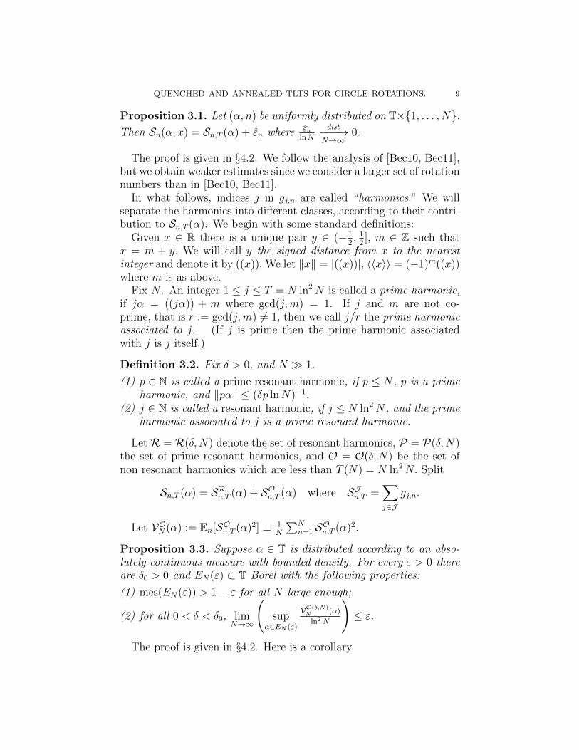
Proposition 3.1. Let (α, n) be uniformly distributed on T×1, . . . , N.Then Sn(α, x) = Sn,T (α) + εn where εn

lnN

dist−−−→N→∞

0.

The proof is given in §4.2. We follow the analysis of [Bec10, Bec11],but we obtain weaker estimates since we consider a larger set of rotationnumbers than in [Bec10, Bec11].

In what follows, indices j in gj,n are called “harmonics.” We willseparate the harmonics into different classes, according to their contri-bution to Sn,T (α). We begin with some standard definitions:

Given x ∈ R there is a unique pair y ∈ (−12, 1

2], m ∈ Z such that

x = m + y. We will call y the signed distance from x to the nearestinteger and denote it by ((x)). We let ‖x‖ = |((x))|, 〈〈x〉〉 = (−1)m((x))where m is as above.

Fix N . An integer 1 ≤ j ≤ T = N ln2N is called a prime harmonic,if jα = ((jα)) + m where gcd(j,m) = 1. If j and m are not co-prime, that is r := gcd(j,m) 6= 1, then we call j/r the prime harmonicassociated to j. (If j is prime then the prime harmonic associatedwith j is j itself.)

Definition 3.2. Fix δ > 0, and N 1.

(1) p ∈ N is called a prime resonant harmonic, if p ≤ N , p is a primeharmonic, and ‖pα‖ ≤ (δp lnN)−1.

(2) j ∈ N is called a resonant harmonic, if j ≤ N ln2N , and the primeharmonic associated to j is a prime resonant harmonic.

Let R = R(δ,N) denote the set of resonant harmonics, P = P(δ,N)the set of prime resonant harmonics, and O = O(δ,N) be the set ofnon resonant harmonics which are less than T (N) = N ln2N. Split

Sn,T (α) = SRn,T (α) + SOn,T (α) where SJn,T =∑j∈J

gj,n.

Let VON (α) := En[SOn,T (α)2] ≡ 1N

∑Nn=1 SOn,T (α)2.

Proposition 3.3. Suppose α ∈ T is distributed according to an abso-lutely continuous measure with bounded density. For every ε > 0 thereare δ0 > 0 and EN(ε) ⊂ T Borel with the following properties:

(1) mes(EN(ε)) > 1− ε for all N large enough;

(2) for all 0 < δ < δ0, limN→∞

(sup

α∈EN (ε)

VO(δ,N)N (α)

ln2N

)≤ ε.

The proof is given in §4.2. Here is a corollary.

10 DMITRY DOLGOPYAT AND OMRI SARIG

Corollary 3.4. For every ε > 0 there is a δ0 > 0 s.t. for all N large

enough and 0 < δ < δ0, Pα,n(|SO(δ,N)n,T |lnN

> ε

)< ε, where 1 ≤ n ≤ N is

distributed uniformly, α ∈ T is sampled from an absolutely continuousmeasure with bounded density, and α, n are independent.

Proof. Without loss of generality 3ε2 < ε. Fubini’s theorem gives

Pα,n

(|SO(δ,N)n,T |lnN

> ε

)≤ ε4 +

∫EN (ε4)

Pn

(|SO(δ,N)n,T |lnN

> ε

)dα.

By Chebyshev’s Inequality, the integrand is less than 1ε2× 1

ln2NVO(δ,N)N .

On EN(ε4), this is less than 2ε2 for all N large enough (uniformly in

α). So Pα,n( 1lnN|SO(δ,N)n,T | > ε) ≤ ε4 + 2ε2 < ε.

Proposition 3.1 and Corollary 3.4 say that the asymptotic distribu-tional behavior of Sn(α) is determined by the behavior of the sum ofthe resonant terms SRn,T (α).

Step 2: An identity for the sum of resonant terms. Let

(3.2) ξj := j〈〈jα〉〉 lnN and Θj(n) := Θ(

[(2n+1)jα+2jx] mod 22

),

where Θ(t) =∞∑k=1

cos(2πkt)

2π2k2, see (2.4).

Proposition 3.5. For all δ small enough,

(3.3)SR(δ,N)n,T

lnN=

∑j∈P(δ,N)

Θj(n) +O(

1lnN

)ξj

.

The big Oh is uniform in j but not in δ.

For the proof, see §4.3.

Step 3: Limit theorems for resonant harmonics. We will use(3.3) to study of the distributional behavior of SRn,T .

First we will describe the distribution of the set of denominatorsξj = j〈〈jα〉〉 lnNj∈P(δ,N), and then we will describe the conditionaljoint distribution of set of numerators, given ξj. Notice that we needinformation on the point process (“random set”) ξj : j ∈ P(δ,N),not just on individual terms.

QUENCHED AND ANNEALED TLTS FOR CIRCLE ROTATIONS. 11

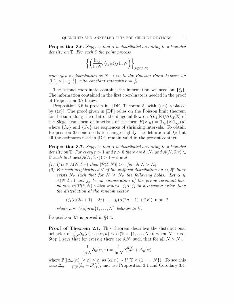
Proposition 3.6. Suppose that α is distributed according to a boundeddensity on T. For each δ the point process(

ln j

lnN, 〈〈jα〉〉j lnN

)j∈P(δ,N)

converges in distribution as N → ∞ to the Poisson Point Process on[0, 1]× [−1

δ, 1δ], with constant intensity c = 6

π2 .

The second coordinate contains the information we need on ξj.The information contained in the first coordinate is needed in the proofof Proposition 3.7 below.

Proposition 3.6 is proven in [DF, Theorem 5] with 〈〈x〉〉 replacedby ((x)). The proof given in [DF] relies on the Poisson limit theoremfor the sum along the orbit of the diagonal flow on SL2(R)/SL2(Z) ofthe Siegel transform of functions of the form F (x, y) = 1IN (x)1JN (y)where IN and JN are sequences of shrinking intervals. To obtainProposition 3.6 one needs to change slightly the definition of IN butall the estimates used in [DF] remain valid in the present context.

Proposition 3.7. Suppose that α is distributed according to a boundeddensity on T. For every r > 1 and ε > 0 there are δ, N0 and A(N, δ, r) ⊂T such that mes(A(N, δ, r)) > 1− ε and

(1) If α ∈ A(N, δ, r) then |P(δ,N)| > r for all N > N0.(2) For each neighborhood V of the uniform distribution on [0, 2]r there

exists NV such that for N ≥ NV the following holds. Let α ∈A(N, δ, r) and jk be an enumeration of the prime resonant har-monics in P(δ,N) which orders ‖jkα‖jk in decreasing order, thenthe distribution of the random vector

(j1(α(2n+ 1) + 2x), . . . , jr(α(2n+ 1) + 2x)) mod 2

where n ∼ Uniform1, . . . , N belongs to V.

Proposition 3.7 is proved in §4.4.

Proof of Theorem 2.1. This theorem describes the distributionalbehavior of 1

lnNSn(α) as (α, n) ∼ U(T × 1, . . . , N), when N → ∞.

Step 1 says that for every ε there are δ,N0 such that for all N > N0,

1

lnNSn(α, x) =

1

lnNSR(δ)n,T + ∆n(α)

where P(|∆n(α)| ≥ ε) ≤ ε, as (α, n) ∼ U(T× 1, . . . , N). To see thistake ∆n := 1

lnN(εn + SOn,T ), and use Proposition 3.1 and Corollary 3.4.

12 DMITRY DOLGOPYAT AND OMRI SARIG

We will prove Theorem 2.1 by showing that 1lnNSR(δ,N)n (α)

dist−−−→N→∞

Cδ

as (α, n) ∼ U(T × 1, . . . , N), where Cδ are random variables such

that Cδdist−−→δ→0

Cauchy.

Let jk be an enumeration of P(δ,N) which orders ‖jkα‖jk in de-creasing order. By step 2,

SR(δ,N)n,T

lnN=∑ Θjk(n) +O( 1

lnN)

ξjk.

Proposition 3.6 says that the point process ξjk converges in law tothe Poisson Point Process on [−1

δ, 1δ]. Proposition 3.7 says that given

ξjk, (Θj1(n)) + O( 1lnN

), . . . ,Θj|P|(n) + O( 1lnN

))dist−−−→N→∞

(Θ1, . . . ,Θ|P|)

where Θi are are independent identically distributed random variableswith distribution (2.6).

It follows thatSR(δ,N)n,T

lnN

dist−−−→N→∞

∑Θmξm

where Θi are independent, dis-

tributed like (2.6), and ξm is a Poisson Point Process Cδ on [−1δ, 1δ]

with density c = 6/π2. In the limit Cδ −−→δ→0

Cauchy random variable,

see Appendix B. This completes the proof of Theorem 2.1 except forthe formula (2.2) which is proven in the appendix.

Proof of Theorem 2.2. Theorem 2.2 describes the convergence indistribution of the (X–valued) random variable

FN(α)(·) :=1

NCard

(1 ≤ n ≤ N : Sn(α,x)

lnN≤ ·)

to FΞ as N → ∞, when α is sampled from an absolutely continuousdistribution on T with bounded density. We will assume for simplicitythat the density is constant, the changes needed to treat the generalcase are routine and are left to the reader.

Again we claim that it is enough to prove the result with SRn,T replac-ing Sn. Let ∆n(α) be as above. By step 1, for every ε there are δ and N0

s.t. for all N > N0, P(|∆n(α)| ≥ ε) ≤ ε as (α, n) ∼ U(T×1, . . . , N).By Fubini’s theorem for such N

mes

(α :

Card(1 ≤ n ≤ N : |∆n(α)| ≥ ε)

N≥√ε

)≤√ε.

It follows that the set of α where the asymptotic distributional behaviorof 1

lnNSRn,T (α) is different from that of 1

lnNSn(α) in the limit N →

∞, δ → 0 has measure zero.

QUENCHED AND ANNEALED TLTS FOR CIRCLE ROTATIONS. 13

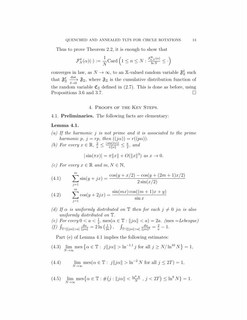
Thus to prove Theorem 2.2, it is enough to show that

F δN(α)(·) :=1

NCard

(1 ≤ n ≤ N :

SRn,T (α)

lnN≤ ·)

converges in law, as N →∞, to an X-valued random variable FδΞ such

that FδΞdist−−→δ→0

FΞ, where FΞ is the cumulative distribution function of

the random variable CΞ defined in (2.7). This is done as before, usingPropositions 3.6 and 3.7.

4. Proofs of the Key Steps.

4.1. Preliminaries. The following facts are elementary:

Lemma 4.1.

(a) If the harmonic j is not prime and it is associated to the primeharmonic p, j = rp, then ((jα)) = r((pα)).

(b) For every x ∈ R, 2π≤ | sin(πx)|

π‖x‖ ≤π2, and

| sin(πx)| = π‖x‖+O(‖x‖3) as x→ 0.

(c) For every x ∈ R and m,N ∈ N,

m∑j=1

sin(y + jx) =cos(y + x/2)− cos(y + (2m+ 1)x/2)

2 sin(x/2)(4.1)

m∑j=1

cos(y + 2jx) =sin(mx) cos((m+ 1)x+ y)

sinx(4.2)

(d) If α is uniformly distributed on T then for each j 6= 0 jα is alsouniformly distributed on T.

(e) For every 0 < a < 12, mes(α ∈ T : ‖jα‖ < a) = 2a. (mes =Lebesgue)

(f)∫T∩[‖jα‖>a]

dα‖jα‖ = 2 ln

(12a

),∫T∩[‖jα‖>a]

dα‖jα‖2 = 2

a− 1.

Part (e) of Lemma 4.1 implies the following estimates:

(4.3) limN→∞

mesα ∈ T : j‖jα‖ > ln−1.1 j for all j ≥ N/ ln10N

= 1,

(4.4) limN→∞

mes(α ∈ T : j‖jα‖ > ln−2N for all j ≤ 2T ) = 1,

(4.5) limN→∞

mesα ∈ T : #

(j : ‖jα‖ < ln6N

N, j < 2T

)≤ ln9N = 1.

14 DMITRY DOLGOPYAT AND OMRI SARIG

We prove (4.5), and leave the proofs of (4.3),(4.4) (which are easier)

to the reader. Let FN denote the set of α in (4.5), then

F cN = α ∈ T :

2T∑j=1

1[‖jα‖< ln6 N

N](α) > ln9N.

By Lemma 4.1(e), the sum has expectation2N ln2N∑j=1

2 ln6NN

. By Markov’s

inequality, mes(F cN) ≤ 1

ln9N

2N ln2N∑j=1

2 ln6NN−−−→N→∞

0.

We also observe the following consequnce of (4.2)

(4.6)

∣∣∣∣∣m∑j=1

cos(y + 2πmx)

∣∣∣∣∣ ≤ min

(π

2||x||,m

).

To see that (4.6) is less than π2||x|| we estimate the numerator of (4.2)

by 1 and the denominator by Lemma 4.1(b). To see that (4.6) is lessthan m, note that each term in the LHS is less than 1 in absolute value.

We note that (4.3) is a very special case of Khinchine’s Theoremon Diophantine approximations (see e.g. [BRV17, Thm 2.3]). Thistheorem says that if ϕ : N→ R+ is a function such that

∑q ϕ(q) <∞,

then for almost every α the inequality

(4.7) ‖qα‖ < ϕ(q)

has only finitely many solutions, while if∑

q ϕ(q) = ∞ and ϕ is non

increasing then (4.7) has infinitely many solutions.Next we list some tightness estimates. Recall that a family of real-

valued functions fn on a probability space (Ω,F ,P) is called tight, iffor every ε > 0 there is an a > 0 s.t. P(|fn| > a) < ε for all n.

Lemma 4.2. Let α ∼ U(T) then

1N lnN

∑Nj=1

1‖jα‖

N∈N

is tight.

Proof. For every ε > 0,

(4.8) mes

(α :

N∑j=1

1

‖jα‖6=

N∑j=1

[1

‖jα‖1[ε/(4N),1/2] (‖jα‖)

])≤ ε

2,

because the event in the brackets equals⋃Nj=1α : ‖jα‖ < ε

4N up to

measure zero, and mesα : ‖jα‖ < ε4N = ε

2Nby Lemma 4.2(e).

QUENCHED AND ANNEALED TLTS FOR CIRCLE ROTATIONS. 15

On the other hand, one can check using Lemma 4.2(f) that

E

(N∑j=1

[1

‖jα‖1[ε/(4N),1/2] (‖jα‖)

])= 2N

(lnN + ln

2

ε

)≤ 3N lnN

if N is sufficiently large. Hence by Markov’s inequality

(4.9) P

(N∑j=1

[1

‖jα‖1[ε/(4N),1/2] (‖jα‖)

]≥ 6N lnN

ε

)≤ ε

2.

Combining (4.8) and (4.9) we see that P(∑N

j=11‖jα‖ ≥

6N lnNε

)≤ ε.

Lemma 4.3. Let α ∼ U(T), then the following families of functionsare tight as N →∞ (recall that T := N ln2N):

(a)1

ln2N

T∑j=1

1

j‖jα‖.

(b)1

(ln lnT )2

T lnβ2 T∑j=T ln−β1 T

1

j‖jα‖1[ln−β3 T,lnβ4 T ](j‖jα‖), for every β1, β2, β3, β4.

(c)1

lnT ln lnT

T∑j=1

1

j‖jα‖1[ln−β3 T,lnβ4 T ](j‖jα‖), for every β3, β4.

We omit the proof, because it is similar to the proof of Lemma 4.2.

4.2. Step 1 (Propositions 3.1 and 3.3). The proofs of these Propo-sitions follow [Bec11] closely, but we decided to give all the details, sinceour assumptions are different.

Proof of Proposition 3.1. The starting point is the Fourier series ex-

pansion of h(x) = x− 12

given in (3.1). Let hT (x) = −T∑j=1

sin(2πjx)

πj.

Summation by parts (see [Bec11, formula (8.6)]) gives us that∣∣∣∣∣n∑k=1

h(x+ kα)−n∑k=1

hT (x+ kα)

∣∣∣∣∣ ≤ 1

T

n∑k=1

1

‖kα‖≤ 1

T

N∑k=1

1

‖kα‖.

The last expression converges to 0 in distribution as α ∼ U(T) andN → ∞, by Lemma 4.2 (recall that T = N ln2N). Thus it suffices tostudy the distribution of

(4.10)n∑k=1

hT (x+ kα)− 1

N

N∑n=1

(n∑k=1

hT (x+ kα)

)

16 DMITRY DOLGOPYAT AND OMRI SARIG

as α ∼ U(T) and N →∞.A direct calculation using Lemma 4.1(c) shows that

(4.10) = Sn,T (α) +T∑j=1

fj

where

fj =1

N

N∑n=1

gj,n =sin(2πjx+ 2πjα)− sin(2πjx+ 2π(N + 1)jα)

4πNj sin2(πjα),

(cf. [Bec11, Lemma 8.2]).Observe that by (4.6) there is a universal constant C such that

(4.11) |fj| ≤ C min

(1

jN‖jα‖2,

1

j‖jα‖

).

Let T := N/ ln10N. By (4.4), with probability close to 1 we have1/(j‖jα‖) < ln2N for all j ≤ T , so with probability close to 1, all j ≤ Tsatisfy ‖jα‖ ∈ [ 1

T ln2N, 1

2]. We split

[1

T ln2N, 1

2

]=[

1T ln2N

, 1N

]∪[

1N, 1

2

]and apply the bounds in (4.11) to each piece. Thus on

(4.12) FN := α : ∀j ≤ T, j‖jα‖ > ln−2Nwe have

T∑j=T+1

|fj| ≤ CT∑

j=T+1

|fj|

where

fj =1[ 1

N, 12

](‖jα‖)Nj‖jα‖2

+

(1[ 1T ln2 N

, 12

](‖jα‖)j‖jα‖

−1[ 1

N, 12

](‖jα‖)j‖jα‖

).

Since by Lemma 4.1(f) Eα(∑T

j=T+1 fj

)≤ C(ln lnN)2, and by (4.4)

mes(FN) −−−→N→∞

1 we conclude that1

lnN

T∑j=T+1

|fj|dist−−−→N→∞

0 as (α, n) ∼

U(T× 1, . . . , N).

Next, we show that1

lnT

T∑j=1

fjdist−−−→N→∞

0. By (4.11),T∑j=1

|fj| ≤ CBN

with BN =T∑j=1

1

Nj‖jα‖2, so it is enough to show that BN

lnN

dist−−−→N→∞

0.

Here is the proof. Split BN = B−N +B+N where the first term contains

the j s.t. j‖jα‖ ≥ δ−1

lnN, and B+

N contains the j s.t. j‖jα‖ < δ−1

lnN.

QUENCHED AND ANNEALED TLTS FOR CIRCLE ROTATIONS. 17

By Lemma 4.1(f)

Eα(B−NlnN

)≤ C

(δT lnN

N lnN

)= O

(1

ln10N

).

Hence by Markov’s inequality 1lnN

B−Ndist−−−→N→∞

0.

Fix ε > 0 and let FN be as in (4.12) above, then (4.4) says thatmes(FN) > 1− ε for all N large enough.

Let R(N) =j ≤ T : δj‖jα‖ lnN ≤ 1

. By Lemma 4.1(a)

(4.13) R(N) ⊂⋃

p∈P(δ,N)

kp : k ∈ Z, p ∈ P(δ,N), kp ≤ T.

Given p ∈ P , let

Rp(δ) := resonant harmonics in R, associated to p.

(4.13) implies that for some constants C,C

B+N ≤

∑p∈P(δ,N)

∑j∈Rp(δ)

C

Nj‖jα‖2

(Lemma 4.1(a))=

∑p∈P(δ,N)

∑kp∈Rp(δ)

C

Nk3p‖pα‖2

≤∑

p∈P(δ,N)

C

Np‖pα‖2

(∞∑k=1

1

k3

)≤

∑p∈P(δ,N)

C

Np‖pα‖2

≤∑

p∈P(δ,N)

C T

N(p‖pα‖)2

(α∈FN )

≤∑

p∈P(δ,N)

C T (ln2N)2

N≤ CCard(P(δ,N))

ln6N.

By Proposition 3.6, if α is distributed according to a bounded densityon T, then Card(P(δ,N)) converges in law as N →∞ to a Poissonianrandom variable. Therefore there is K(ε) so that

mesα ∈ T : Card(P(δ,N)) ≤ K(ε) > 1− ε.

It follows that mesα ∈ T : B+N ≤ K(ε)C ln−6N > 1 − 2ε, whence

1lnN

B+N

dist−−−→N→∞

0.

To summarize,

εN := Sn(α, x)−Sn,T (α) =T∑j=1

fj+error which tends to 0 in distribution,

and1

lnN

T∑j=1

|fj| =1

lnN

T∑j=T+1

|fj|+B−N +B+N

dist−−−→N→∞

0 by the ar-

guments above.

18 DMITRY DOLGOPYAT AND OMRI SARIG

Proof of Proposition 3.3. We give the proof assuming that α ∼ U(T).The modifications needed to deal with absolutely continuous measureswith bounded densities are routine, and are left ot the reader.

Simple algebra gives VON = 1N

∑j∈O

N∑n=1

g2j,n + 1

N

∑j1,j2∈Oj1 6=j2

gj1,ngj2,n, where

gj,n = cos((2n+1)πjα+2πjx)2πj sin(πjα)

. To bound the sum of diagonal terms, we use

that by (4.6) |gj,n| < 1j‖jα‖ , whence

(4.14)1

N

∑j∈O

N∑n=1

g2j,n ≤

∑j∈O

1

N

N∑n=1

1

j2‖jα‖2=: Diag(N).

To bound the sum of off-diagonal terms, we first collect terms to get

1

N

∑j1,j2∈Oj1 6=j2

gj1,ngj2,n =∑

j1,j2∈Oj1 6=j2

1

4π2j1j2 sin(πj1α) sin(πj2α)Γj1,j2,N ,

where

Γj1,j2,N :=1

N

N∑n=1

cos((2n+ 1)πj1α + 2πjx) cos((2n+ 1)πj2α + 2πjx).

Now the identity cos A+B2

cos A−B2

= 12[cosA+ cosB] and (4.6) give

Γj1,j2,N ≤ C[min

(1

N‖(j1−j2)α‖ , 1)

+ min(

1N‖(j1+j2)α‖ , 1

)].

This and the estimate j| sin(πjα)| ≥ 2j‖jα‖ (Lemma 4.1(b)) impliesthat for some universal constant C

1

N

∑j1,j2∈Oj1 6=j2

gj1,ngj2,n ≤ C[OffDiag−(N) + OffDiag+(N)

]where

(4.15) OffDiag± :=∑

j1,j2∈Oj1 6=j2

min(

1N‖(j1±j2)α‖ , N‖(j1 ± j2)α‖

)j1‖j1α‖ · j2‖j2α‖

.

Since min(x, x−1) ≤ 1 for all x, the numerator is bounded by one.Thus VON ≤ Diag(N)+C[OffDiag−+OffDiag+]. We need the follow-

ing additional decomposition:

(4.16) OffDiag± := OffDiag±i + OffDiag±ii + OffDiag±iii + OffDiag±iv

where

(i) OffDiag−i : sum over the terms s.t. ‖(j1 − j2)α‖ ≥ ln6NN

;

QUENCHED AND ANNEALED TLTS FOR CIRCLE ROTATIONS. 19

(ii) OffDiag−ii : ‖(j1 − j2)α‖ ≤ ln6NN

, and j1‖j1α‖ ≥ ln10N ;

(iii) OffDiag−iii: ‖(j1 − j2)α‖ ≤ ln6NN

, and

j1‖j1α‖ ≤ ln10N, j2‖j2α‖ ≥ ln10N ;

(iv) OffDiag−iv: ‖(j1 − j2)α‖ ≤ ln6NN

,

j1‖j1α‖ ≤ ln10N, j2‖j2α‖ ≤ ln10N.

Similarly for OffDiag+ with ‖(j1 + j2)α‖ instead of ‖(j1 − j2)α‖.We now have the following upper bound

(4.17) VON ≤ Diag + Civ∑k=i

(OffDiag−k + OffDiag+

k

).

For every ε > 0, and for each of the nine summands D1, . . . , D9 above,we will construct δ0 > 0 and Borel sets A1(ε,N), . . . , A9(ε,N) ⊂ T s.t.mes[Ai] > 1− ε

9, and with the following property:

(4.18) ∀0 < δ < δ0, limN→∞

(supα∈Ai

Di

ln2N

)≤ ε

9.

This will prove the proposition, with EN(ε) :=9⋂i=1

Ai.

We begin by recalling some facts on the typical behavior of ‖jα‖ forα ∼ U(T). Recall that T := N ln2N , and let

E∗N :=

α ∈ T :

(A) ∀j > Nln10N

, j‖jα‖ > ln−1.1 j(B) ∀j ≤ 2T, j‖jα‖ > ln−2N

(C) #1 ≤ j ≤ 2T : ‖jα‖ < ln6NN ≤ ln9N

.

Then mes(E∗N) −−−→N→∞

1, by (4.3),(4.4), and (4.5). Most of our sets Ai

will be subsets of E∗N .

The summand Diag =∑

j∈O1N

∑Nn=1

1j2‖jα‖2 .

Suppose α ∈ E∗N . By the definition of resonant harmonics, for everyj ∈ O either δj‖jα‖ lnN ≥ 1, or N ≤ j ≤ T.

20 DMITRY DOLGOPYAT AND OMRI SARIG

In the first case, j‖jα‖ ≥ (δ lnN)−1. In the second case, by property(A) of E∗N , j‖jα‖ > ln−1.1 j ≥ ln−1.1 T . Accordingly,

Eα(Diag · 1E∗N ) ≤

[N∑j=1

∫T

1

j2‖jα‖21[j‖jα‖>(δ lnN)−1]dα

+T∑

j=N+1

∫T

1

j2‖jα‖21[j‖jα‖>ln−1.1 T ]dα

]

≤

[N∑j=1

2δj lnN

j2+

T∑j=N+1

2j ln1.1 T

j2

](by Lemma 4.1(f))

≤ 2δ ln2N + 4 ln1.1N ln lnN.

Let δ0 := ε2/1000, and choose N0 so large that for all N > N0,

mes(E∗N) > 1− ε/9 and 4 ln1.1N ln lnNln2N

< ε2/1000. By Markov’s inequal-ity, for all N > N0 and δ < δ0,

mesα ∈ E∗N : Diag > ε9

ln2N ≤ 2δ ln2N + 4 ln lnN

(ε/9) ln2N<ε

9.

We obtain (4.18) with Di = Diag, Ai := α ∈ E∗N : Diag ≤ ε9

ln2N,and δ0 := ε2/1000. Notice that this Ai depends on ε.

The summand OffDiag−i : This is the part of (4.15) with j1, j2 s.t.

‖(j1 − j2)α‖ ≥ ln6NN

.

OffDiag−i ≤∑

j1,j2∈O

1/ ln6N

j1‖j1α‖ · j2‖j2α‖

≤ 1

ln6N

(T∑j=1

1

j‖jα‖

)2

=1

ln2N

(1

ln2N

T∑j=1

1

j‖jα‖

)2

.

By Lemma 4.3(a), the term in the brackets is tight: there is a constant

K = K(ε) s.t. for all N , A := α ∈ T : 1ln2N

∑Tj=1

1j‖jα‖ ≤ K has

measure more than 1− ε9.

For all N > exp 4

√9K2

ε, for every α ∈ A, 1

ln2NOffDiag−i ≤ K2

ln4N< ε

9,

and we get (4.18) with Ai = A, N0 = exp 4

√9K2

ε.

The summand OffDiag−ii : Suppose α ∈ E∗N , and let j2 ∈ O be anindex which appears in OffDiag−ii . Let I(j2) be the set of j1 s.t. (j1, j2)appear in OffDiag−ii , namely

I(j2) := j1 ∈ O : ‖(j1 − j2)α‖ ≤ ln6NN, j1‖j1α‖ ≥ ln10N.

QUENCHED AND ANNEALED TLTS FOR CIRCLE ROTATIONS. 21

By property (C) in the definition of E∗N (applied to |j1 − j2|), thecardinality of I(j2) is bounded by 2 ln9N .

Since the numerator in (4.15) is bounded by one, and since in case(ii) j1‖j1α‖ ≥ ln10N , we have

OffDiag−iiln2N

≤ 1

ln2N

T∑j2=1

1

j2‖j2α‖

∑j1∈I(j2)

1j1‖j1α‖

≤ 1

ln2N

T∑j2=1

1

j2‖j2α‖

(|I(j2)|ln10N

)≤ 2

ln3N

T∑j=1

1

j‖jα‖=

2

lnN

(1

ln2N

T∑j=1

1j‖jα‖

).

The term in the brackets is tight by Lemma 4.3(a), and we can continueto obtain (4.18) as we did in case (i).

The summand OffDiag−iii: This is similar to OffDiag−ii .

The summand OffDiag−iv: Suppose the pair of indices (j1, j2) appears

in OffDiag−iv: ‖(j1− j2)α‖ ≤ ln6NN

, j1‖j1α‖ ≤ ln10N , j2‖j2α‖ ≤ ln10N .Let jmax := max(j1, j2) and jmin := min(j1, j2).

We claim that if α ∈ E∗N , then

ln−2N ≤jmin‖jminα‖ ≤ ln10N ;(4.19)

ln−1.1 T ≤jmax‖jmaxα‖ ≤ ln10N ;(4.20)

jmax ≥N

ln8N.(4.21)

Here is the proof. The left side of (4.19) is because jmin ≤ T := N ln2Nby definition of O and by property (B) in the definition of E∗N . Theright side is because we are in case (iv). Let ∆j := jmax − jmin, then∆j ≤ jmax ≤ T , whence by property (B), ∆j‖(∆j)α‖ > ln−2N . So

∆j > (‖(∆j)α‖ ln2N)−1. In case (iv), ‖(∆j)α‖ ≤ ln6NN

, so ∆j ≥ Nln8N

.Since jmax ≥ ∆j, (4.21) follows. The right side of (4.20) is by thedefinition of case (iv). The left side is because of (4.21), property (A)in the definition of E∗N , and because jmax ≤ T .

We can now see that for every α ∈ E∗N ,

OffDiag−iv(N)

ln2N≤

2

ln2N

T∑j= N

ln8 N

1

j‖jα‖1[ln−1.1 T≤j‖jα‖≤ln10N ]

( T∑j=1

1

j‖jα‖1[ln−2 T≤j‖jα‖≤ln10N ]

)

22 DMITRY DOLGOPYAT AND OMRI SARIG

≤ 2(ln lnT )3 lnT

ln2N×

1

(ln lnT )2

T∑j= T

ln10 T

1

j‖jα‖1[ln−1.1 T≤j‖jα‖≤ln10N ]

××

(1

lnT ln lnT

T∑j=1

1

j‖jα‖1[ln−2 T≤j‖jα‖≤ln10N ]

).

The first term tends to zero (because T = N ln2N), and the secondand third terms are tight by Lemma 4.3(b),(c). We can now proceedas before to obtain (4.18) for Di = OffDiag−iv.

The summands OffDiag+k , k = i, . . . , iv: These can be handled in

the same way as OffDiag−k , except that in cases (ii),(iii) and (iv) weneed to apply properties (B) and (C) to j1 +j2 instead of |j1−j2|. Thisis legitimate since j1 + j2 ≤ 2T .

4.3. Step 2 (Proposition 3.5).

Proof of Proposition 3.5. Fix δ > 0 small, α ∈ T \Q, and N 1, andset P = P(δ,N),R = R(δ,N). Recall that

Rp(δ) := resonant harmonics in R, associated to p.Then we have the following decomposition for SRn,T/ lnN

(4.22)SRn,TlnN

≡ 1

lnN

∑j∈R

gj,n =1

lnN

∑p∈P

∑kp∈Rp(δ)

cos((kp)tn)

2πkp sin(πkpα).

where

(4.23) tn = (2n+ 1)πα + 2πx

To continue, we need the following observations on Rp(δ):

Claim 1: Suppose p ∈ P , and Lp := min(b12δp lnNc, bN ln2N/pc).

For every 1 ≤ k ≤ Lp

(a) kp ∈ Rp(δ) and ((kpα)) = k((pα));(b) 1

2πkp sin(πkpα)= 1

p〈〈pα〉〉

(1

2π2k2+O (‖pα‖2)

).

Proof: Write pα = m+ ((pα)) with m ∈ Z. If j = kp with 1 ≤ k ≤ Lp,then jα = km+ k((pα)) and, since p is prime resonant,

|k((pα))| = k‖pα‖ ≤ Lp(δp lnN)−1 ≤ 1

2.

Since α is irrational, this is a strict inequality, whence ((jα)) = k((pα)).This also shows that jα = km+ ((jα)) whence r := gcd(j, km) = k,

and j is associated to p ≡ j/r. To complete the proof that j ∈ Rp(δ)

QUENCHED AND ANNEALED TLTS FOR CIRCLE ROTATIONS. 23

we just need to check that j ≤ N ln2N . This is immediate from thedefinition of Lp. This proves (a).

For (b), we write again pα = m + ((pα)) with m ∈ Z and note thatsin(πkpα) = sin(πkm+π((kpα))) = (−1)m sin π((kpα)). We saw abovethat if k ≤ Lp, then ((kpα)) = k((pα)). So

sin(πkpα) = (−1)m sin πk((pα)) = (−1)mπk((pα)) +O(k3‖pα‖3).

Note that (−1)m((pα)) = 〈〈pα〉〉 because of the decomposition pα =m+ ((pα)) above. So sin(πkpα) = πk〈〈pα〉〉+O(k3‖pα‖3). Thus

1

2πkp sin(πkpα)=

1

2π2k2p〈〈pα〉〉 (1 +O (k2||pα||3))=

1 +O (k2||pα||3)

2π2k2p〈〈pα〉〉proving (b).

Claim 2: If p ∈ P and kp ∈ Rp(δ), then 12πkp sin(πkpα)

= O(

1k2p‖pα‖

).

Proof: Write kpα = ` + ((kpα)) with ` ∈ Z. Since p is associated tokp, gcd(kp, `) = k. We have

‖kpα‖ = |kpα− `| = gcd(kp, `)

∣∣∣∣ kp

gcd(kp, `)α− `

gcd(kp, `)

∣∣∣∣= k

∣∣∣∣pα− `

gcd(kp, `)

∣∣∣∣ ≥ k‖pα‖.

In particular, k‖pα‖ ≤ ‖kpα‖ ≤ 12. Therefore ‖kpα‖ = k‖pα‖, and

| sin(πkpα)| π‖kpα‖ = πk‖pα‖, whence 12πkp sin(πkpα)

= O(

1k2p‖pα‖

).

Claim 3: Suppose p ∈ P , then

kp : k = 1, . . . , Lp ⊂ Rp(δ) ⊂kp : k = 1, . . . ,

N ln2N

p

.

Proof: The first inclusion is by Claim 1(a), the second is because bydefinition, every j ∈ R is less than T = N ln2N .

We now return to (4.22). Claims 2 and 3 say that the inner sum is∑kp∈Rp(δ)

gkp,n =

Lp∑k=1

gkp,n+O

1

p‖pα‖

N ln2N/p∑k=Lp+1

1

k2

. If Lp = bN ln2N/pc,

then the error term vanishes. If not, then Lp = b12δp lnNc and the er-

ror term can be found by summation to be equal to O(

1δp‖pα‖ ·

1p lnN

).

Thus∑

kp∈Rp(δ) gkp,n =∑Lp

k=1 gkp,n + O(

1p‖pα‖ ·

1p lnN

)(where the im-

plied constant is not uniform in δ).

24 DMITRY DOLGOPYAT AND OMRI SARIG

Applying Claim 1 to∑Lp

k=1 gkp,n we obtain (recall (4.23))

SRn,TlnN

=1

lnN

∑p∈P

1

p〈〈pα〉〉

(Lp∑k=1

(cos((kp)tn)

2π2k2+O(‖pα‖2)

)+O

(1

p lnN

))

=1

lnN

∑p∈P

1

p〈〈pα〉〉

(Lp∑k=1

cos((kp)tn)

2π2k2+O(‖pα‖2Lp) +O

(1

p lnN

)).

For p ∈ P , ‖pα‖ < 1δp lnN

, so ‖pα‖2Lp ≤12δp lnN

δ2p2 ln2N= O

(1

p lnN

). Thus

SRn,TlnN

=∑p∈P

1

p〈〈pα〉〉 lnN

(Lp∑k=1

cos((kp)tn)

2π2k2+O

(1

p lnN

)).

Every p ∈ P satisfies p ≤ N . So Lp ≥ min(b12δp lnNc, bln2Nc), whence

∞∑k=Lp+1

cos((kp)tn)

2π2k2= O

(1

p lnN

). So

SRn,TlnN

=∑p∈P

1

p〈〈pα〉〉 lnN

(∞∑k=1

cos(k(ptn))

2π2k2+O

(1

lnN

)).

This is equation (3.3).

4.4. Step 3 (Proposition 3.7).

Proof of Proposition 3.7. We carry out the proof assuming α ∼ U(T),and the leave the routine modifications needed to treat the general caseto the reader. Fix an integer r > 1 and a small real number ε > 0.

Claim 1: There exist δ > 0, N0 ≥ 1 s.t. for all N > N0, Ω(N, δ, r) :=α ∈ T : |P(δ,N)| ≥ r has measure bigger than 1− ε.Proof: Proposition 3.6 says that j〈〈jα〉〉 lnN : j ∈ P(δ,N) convergesas a point process to a Poisson point process with density 6

π2 on [−1δ, 1δ].

So #P(δ,N)dist−−−→N→∞

Poisson distribution with expectation 12π2δ

. If we

choose δ small enough, the probability that this random variable is lessthan 2r is smaller than ε

2. So the claim holds with some N0.

Let µα,r,N := 1N

∑Nn=1 δ(j1tn,...,jrtn) where tn = (2n + 1)πα + 2πx (see

(4.23)) and fix some weak-star open neighborhood V of the normalizeduniform Lebesgue on [0, 2]r. We will construct NV s.t. for all N ≥ NV,

mes (α ∈ Ω(N, δ, r) : µα,r,N ∈ V) > 1− 2ε

where jk := jk(α, δ,N) enumerate P(δ,N) as in Proposition 3.7.

QUENCHED AND ANNEALED TLTS FOR CIRCLE ROTATIONS. 25

Without loss of generality, V =⋂ν0ν=1µ : |

∫[0,2]r

fνdµ| < ε where

ε > 0, ν0 ∈ N, and fν(x1, . . . , xr) = eiπ∑rk=1 l

(ν)k xk , where

l(ν) := (l(ν)1 , . . . , l(ν)

r ) ∈ Zr \ 0 (1 ≤ ν ≤ ν0).

This is because any weak star open neighborhood of Lebesgue’s mea-sure on [0, 2]r contains a neighborhood of this form. Let

Lν := Lν(α, δ,N) :=r∑

k=1

l(ν)k jk.

Claim 2: mes (α ∈ Ω(N, δ, r) : Lν = 0 for some 1 ≤ ν ≤ ν0) −−−→N→∞

0.

Proof. Proposition 3.6 says that the sequence jk is superlacunary inthe sense that for each R

(4.24) mes

(α : ∀1 ≤ k′ < k′′ ≤ r :

max(jk′ , jk′′)

min(jk′ , jk′′)≥ R

)−−−→N→∞

1.

To see this recall that the gaps between neighboring points of a Poissonprocess have an exponential distribution, therefore for any ε there existsδ such that the gaps between ln jk′ and ln jk′′ are, with probability 1−ε,bounded below by δ lnN.

Let k∗ν = arg max(jk : l(ν)k 6= 0). Applying (4.24) with

R = Rν := 2(r − 1)∑k

|l(ν)k |

we see that for all N large enough, with almost full probability, jk∗ν ≥2∑k 6=k∗|l(ν)k jk|, whence Lν 6= 0. This proves the claim.

Notice that this argument also shows that with almost full probabil-

ity, |Lν | ≤ 2l(ν)k∗ jk∗ν .

Claim 3: mes(α ∈ Ω(N, δ, r) : ∃ν ≤ ν0 s.t. ‖Lνα/2‖ ≤ lnN

N

)−−−→N→∞

0.

Proof. By Proposition 3.6, ln jlnN

: j ∈ P(δ,N) converges as a point

process to a Poisson point process with intensity 12π2δ

on [0, 1], therefore

mes(α ∈ Ω(N, δ, r) : jk∗ν >

Nln4N

)≤ mes

(α ∈ T : ∃j ∈ P(δ,N) s.t. ln j

lnN> 1− 4 ln lnN

lnN

)−−−→N→∞

0.

Therefore for allN large enough, with almost full probability in Ω(N, δ, r),jk∗ν ≤ N/ ln4N , whence (for N large enough) also

1 ≤ |Lν | ≤ 2lk∗νjk∗ν <N

ln4Nmaxν‖l(ν)‖∞ <

N

ln3N.

26 DMITRY DOLGOPYAT AND OMRI SARIG

A simple modification of (4.4) gives

mes(α ∈ T : j‖jα/2‖ > ln−2N for all 1 ≤ j ≤ N) −−−→N→∞

1.

It follows that for all N large enough, with almost full probability inΩ(N, δ, r), Lν‖Lνα/2‖ > 1/ ln2N , whence

‖Lνα/2‖ >1

Lν ln2N>

1N

ln3N· ln2N

=lnN

N,

proving the claim.

Fix NV s.t. for every N > NV, for each 1 ≤ ν ≤ ν0, ‖Lνα/2‖ >lnN/N with almost full probability in Ω(N, δ, r). Make NV so largethat 1

lnNV< ε. Then for every N > NV∣∣∣∣∫ fνdµα,r,N

∣∣∣∣ =1

N

∣∣∣∣∣N∑n=1

eπiLν(α(2n+1)+2x)

∣∣∣∣∣ ≤ 1

N

2

|1− e2πiLνα|

=1

N‖Lα/2‖≤ 1

N · lnNN

=1

lnN< ε,

whence µα,r,N ∈ V as required.

Appendix A. Proof of proposition 1.1

Suppose f : T → R is differentiable on T \ x1, . . . , xN, and f ′

extends to a function of bounded variation on T. Since f ′ has boundedvariation, f ′ is bounded. So f is Lipschitz between its singularities. Itfollows that L−i := lim

t→x−if(t), L+

i := limt→x+i

f(t) exist for each i.

Let ϕ(t) := f(t)−∑N

i=1(L+i −L−i )h(t+ x1)−

∫T f(s)ds. It is easy to

see that ϕ|T\x1,...,xN extends to a continuous function ψ on T s.t.

ψ(t) = f(t)−N∑i=1

(L+i − L−i )h(t+ x1)−

∫Tf(s)ds

for every t ∈ T \ x1, . . . , xN. (But maybe the identity breaks at xi.)By construction, ψ ∈ C(T) and ψ′|T\x1,...,xN = f ′|T\x1,...,xN extends

to a function with bounded variation on T.Expand ψ to a Fourier series: ψ(x) =

∑k∈Z−0

ake2πikx.Our assumptions

imply ak = O(k−2). A formal solution of ψ = κα − κα Rα gives

κα(x) ∼∑

k∈Z\0

bk,αe2πikx, where bk,α =

ak1− e2πikα

.

QUENCHED AND ANNEALED TLTS FOR CIRCLE ROTATIONS. 27

We claim that for a.e. α,∑k

|bk,α| <∞ so that κα is a well-defined

continuous function. Indeed bk,α = O(|ak|||kα||

)= O

(1

k2||kα||

)so it suf-

fices to check that∞∑k=1

1

k2||kα||converges for a.e. α.

By Khinchine theorem for a.e. α we have ||kα|| > k−1.1 for all large

k, so∞∑k=1

1

k2||kα||converges for a.e. α iff

∞∑k=1

1

k2||kα||1[||kα||>k−1.1]

converges for a.e. α. This is indeed the case, because∫T

∞∑k=1

1

k2||kα||1[||kα||>k−1.1]dα =

∑ 1

k2· 2 ln

(k1.1

2

)<∞.

Appendix B. Cauchy and Poisson.

Let Ξ = ξn be a Poisson process on R with intensity c and let Θn

be i.i.d bounded random variables with zero mean independent of Ξ.Note that the set of pairs (ξm,Θm) forms a marked Poisson process

on R × R (see [LP, Section 5.3] for background on marked Poissonprocesses). Accordingly one can apply the exponential formula formarked Poisson processes ([LP, page 42]) which says that if u is abounded continuous function on [L1, L2]× R and t ∈ R then

(B.1) E

exp∑

ξm∈[L1,L2]

tu(ξm,Θm)

=

exp

[c

∫ L2

L1

EΘ

(etu(y,Θ) − 1

)dy

].

Note that computing the first and second derivative of (B.1) with re-spect to t at t = 0 we obtain

(B.2) E

∑ξm∈[L1,L2]

u(ξm,Θm)

= c

∫ L2

L1

EΘ (u(y,Θ)) dy

(B.3) E

∑ξm∈[L1,L2]

u2(ξm,Θm)

= c

∫ L2

L1

EΘ

(u2(y,Θ)

)dy

28 DMITRY DOLGOPYAT AND OMRI SARIG

Now consider

YL =∑|ξn|<L

Θn

ξn.

Our goal is to compute the distributional limit of YL as L→∞. Rewrite

YL =∑ξ∗n<L

Θ∗nξ∗n

where ξ∗n = |ξn|, Θ∗n = |ξn|ξn

Θn. Note that ξ∗n is a Poisson

process on R+ with intensity 2c, |Θ∗n| = |Θn| and the distribution of Θ∗

is symmetric. Let F be the distribution function of Θ∗ and ϕ(t) be itscharacteristic function. Note that ϕ is real, namely, ϕ(t) = E(cos(tΘ∗))because Θ∗ is symmetric. Let ΦL(t) be the characteristic function ofYL. Applying (B.1) with uε(ξ,Θ) = i Θ

max(ξ,ε)and letting ε to 0 we

obtain

ΦL(t) = exp

[2c

∫ L

0

(ϕ(t/y)− 1) dy

].

where the factor 2 appears because the intensity of ξ∗m is 2c.Introducing x = 1/y, δ = 1/L we can rewrite this expression as

ΦL(t) = exp

[2c

∫ ∞δ

ϕ(xt)− 1

x2dx

].

The integral in the above expression equals to

Rδ(t) =

∫ ∞δ

∫ K

−K

cos(xtθ)− 1

x2dxdF (θ)

where K = ||Θ||∞. Using that the cosine function is even we obtain∫ ∞δ

cos(xtθ)− 1

x2dx = |tθ|

∫ ∞δ|tθ|

cos(x)− 1

x2dx

= |tθ|∫ ∞

0

cos(x)− 1

x2dx+O (δtθ) = −π|t||θ|

2+O (δtθ) .

Integrating with respect to θ and using that E(|Θ∗|) = E(|Θ|) we seethat

limδ→0

Rδ(t) = −π|t|2

E(|Θ|).

HencelimL→∞

ΦL(t) = exp (−cπ|t|E(|Θ|)) .

It follows that YL converges as L→∞ to ρ2C where

(B.4) ρ2 = cπE(|Θ|)and C is the standard Cauchy distribution with density 1

π(1+x2).

In particular, for Θ defined by (2.4) it follows from (2.5) that

QUENCHED AND ANNEALED TLTS FOR CIRCLE ROTATIONS. 29

(B.5) E(|Θ|) =1

2

∫ 1

0

∣∣∣∣θ2 − θ +1

6

∣∣∣∣ dθ =1

18√

3.

Combining (B.4), (2.8) and (B.5) we get (2.2).

References

[ADDS15] Artur Avila, Dmitry Dolgopyat, Eduard Duryev, and Omri Sarig. Thevisits to zero of a random walk driven by an irrational rotation. IsraelJ. Math., 207(2):653–717, 2015.

[Bec10] Jozsef Beck. Randomness of the square root of 2 and the giant leap,Part 1. Period. Math. Hungar., 60(2):137–242, 2010.

[Bec11] Jozsef Beck. Randomness of the square root of 2 and the giant leap,Part 2. Period. Math. Hungar., 62(2):127–246, 2011.

[BRV17] Victor Beresnevich, Felipe Ramirez, and Sanju Velani. Metric diophan-tine approximation: aspects of recent work. London Math. Soc. Lect.Notes, 437:1–95, 2017.

[BU] Michael Bromberg and Corinna Ulcigrai. A temporal central limit theo-rem for real-valued cocycles over rotations. preprint ArXiv:1705.06484.

[CGZ00] Francis Comets, Nina Gantert, and Ofer Zeitouni. Quenched, annealedand functional large deviations for one-dimensional random walk in ran-dom environment. Probab. Theory Related Fields, 118(1):65–114, 2000.

[DF] Dmitry Dolgopyat and Bassam Fayad. Deviations of ergodic sums fortoral translations: Boxes. preprint, arXiv:1211.4323.

[DF15] Dmitry Dolgopyat and Bassam Fayad. Limit theorems for toral trans-lations. In Hyperbolic dynamics, fluctuations and large deviations, vol-ume 89 of Proc. Sympos. Pure Math., pages 227–277. Amer. Math. Soc.,Providence, RI, 2015.

[DG12] Dmitry Dolgopyat and Ilya Goldsheid. Quenched limit theorems fornearest neighbour random walks in 1D random environment. Comm.Math. Phys., 315(1):241–277, 2012.

[DS17] Dmitry Dolgopyat and Omri Sarig. Temporal distributional limit the-orems for dynamical systems. J. Statistical Physics, 166(3-4):680–713,2017.

[Her79] Michael Robert Herman. Sur la conjugaison differentiable des

diffeomorphismes du cercle a des rotations. Inst. Hautes Etudes Sci.Publ. Math., (49):5–233, 1979.

[Jar29] Vojtech Jarnık. Zur metrischen theorie der diophantischen approxima-tionen. Prace Matematyczno-Fizyczne, 36(1):91–106, 1928-1929.

[Kes60] Harry Kesten. Uniform distribution mod 1. Ann. of Math. (2), 71:445–471, 1960.

[Kes62] Harry Kesten. Uniform distribution mod 1. II. Acta Arith, 7:355–380,1961/1962.

[Khi24] Alexander Ya. Khintchine. Einige Satze uber Kettenbruche, mit An-wendungen auf die Theorie der Diophantischen Approximationen. Math.Ann., 92(1-2):115–125, 1924.

30 DMITRY DOLGOPYAT AND OMRI SARIG

[LP] Gunter Last and Mathew Penrose. Lectures on Poisson process. Instituteof Mathematical Statistics Textbooks.

[PS13] Jonathon Peterson and Gennady Samorodnitsky. Weak quenched limit-ing distributions for transient one-dimensional random walk in a randomenvironment. Ann. Inst. Henri Poincare Probab. Stat., 49(3):722–752,2013.

Department of Mathematics, University of Maryland at CollegePark, College Park, MD 20740, USA

E-mail address: dmitry@math.umd.edu

Faculty of Mathematics and Computer Science, The Weizmann In-stitute of Science, POB 26, Rehovot, Israel

E-mail address: omsarig@gmail.com