


γλώσσες
Σελίδες
Νομικός

Quadrature By Zeta CorrectionA Singular Quadrature Method For Integral Equations
Bowei (Bobbie) WuPer-Gunnar Martinsson
Sayas Numerics SeminarFeb. 23, 2021
Outline
1. Integral Equations And Singular Quadrature
2. Zeta Quadrature On Curves And Surfaces
2/14
Integral Equation Method
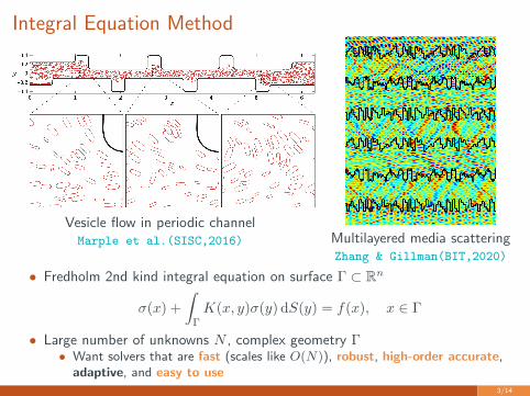
Vesicle flow in periodic channelMarple et al.(SISC,2016) Multilayered media scattering
Zhang & Gillman(BIT,2020)
• Fredholm 2nd kind integral equation on surface Γ ⊂ Rn
σ(x) +
∫Γ
K(x, y)σ(y) dS(y) = f(x), x ∈ Γ
• Large number of unknowns N , complex geometry Γ• Want solvers that are fast (scales like O(N)), robust, high-order accurate,
adaptive, and easy to use3/14
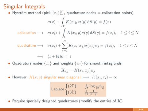
Singular Integrals• Nystrom method (pick {xi}Ni=1 quadrature nodes = collocation points)
σ(x) +
∫Γ
K(x, y)σ(y) dS(y) = f(x)
collocation −→ σ(xi) +
∫Γ
K(xi, y)σ(y) dS(y) = f(xi), 1 ≤ i ≤ N
quadrature −→ σ(xi) +
N∑j=1
K(xi, xj)σ(xj)wj = f(xi), 1 ≤ i ≤ N
−→ (I + K)σ = f
• Quadrature nodes {xi} and weights {wi} for smooth integrands
Ki,j = K(xi, xj)wj
• However, K(x, y) singular near diagonal =⇒ K(xi, xi) =∞
Laplace
{(2D) 1
2π log 1|x−y|
(3D) 14π
1|x−y|
• Require specially designed quadratures (modify the entries of K)
4/14

Singular Quadrature By Correcting The Regular
• global vs panel quadrature
• global vs local correction
• on-grid vs off-grid (auxiliary nodes) correction
• Compatibility with fast algorithms
• Fast Multipole Method (FMM)(I+K)σ in O(N) time
Fast Direct Solver (FDS)(I+K)−1f in O(N) time
• FMM/FDS-compatible:Ki,j = K(xi, xj)wj except for O(N) entries
Martinsson (SIAM,2019)5/14
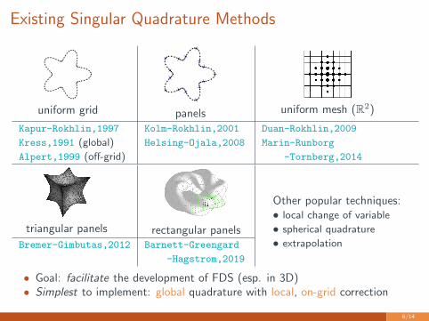
Existing Singular Quadrature Methods
uniform grid panels uniform mesh (R2)
Kapur-Rokhlin,1997 Kolm-Rokhlin,2001 Duan-Rokhlin,2009
Kress,1991 (global) Helsing-Ojala,2008 Marin-Runborg
Alpert,1999 (off-grid) -Tornberg,2014
triangular panels rectangular panels
Other popular techniques:• local change of variable
• spherical quadrature
• extrapolationBremer-Gimbutas,2012 Barnett-Greengard
-Hagstrom,2019
• Goal: facilitate the development of FDS (esp. in 3D)• Simplest to implement: global quadrature with local, on-grid correction
6/14
Outline
1. Integral Equations And Singular Quadrature
2. Zeta Quadrature On Curves And Surfaces
7/14
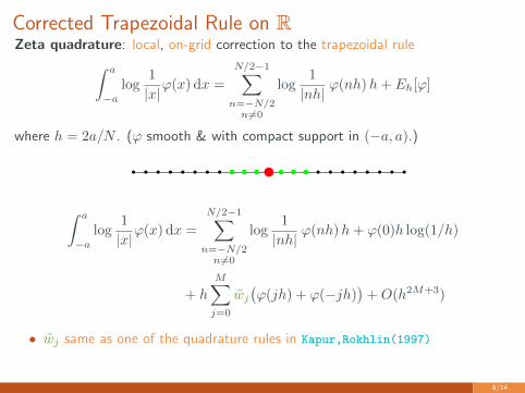
Corrected Trapezoidal Rule on RZeta quadrature: local, on-grid correction to the trapezoidal rule∫ a
−alog
1
|x|ϕ(x) dx =
N/2−1∑n=−N/2n 6=0
log1
|nh|ϕ(nh)h+ Eh[ϕ]
where h = 2a/N . (ϕ smooth & with compact support in (−a, a).)
∫ a
−alog
1
|x|ϕ(x) dx =
N/2−1∑n=−N/2n6=0
log1
|nh|ϕ(nh)h+ ϕ(0)h log(1/h)
+ h
M∑j=0
wj(ϕ(jh) + ϕ(−jh)
)+O(h2M+3)
• wj same as one of the quadrature rules in Kapur,Rokhlin(1997)
8/14
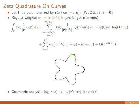
Zeta Quadrature On Curves• Let Γ be parameterized by r(x) on [−a, a). (WLOG, r(0) = 0)
• Regular weights wn = |r′(nh)|h (arc length elements)∫Γ
log1
|r|ϕ(r) ds =
N/2−1∑n=−N/2n 6=0
log1
|r(nh)|ϕ(r(nh))wn + ϕ(0)w0 log(1/w0)
+
M∑j=0
wj(ϕ(jh)wj + ϕ(−jh)w−j
)+O(h2M+3)
• Geometric analysis: log |r(x)| ≈ log |r′(0)x| for x ≈ 0
9/14
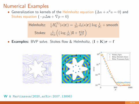
Numerical Examples• Generalization to kernels of the Helmholtz equation (∆u+ κ2u = 0) and
Stokes equation (−µ∆u +∇p = 0)
Helmholtz: i4H
(1)0 (κ|r|) = 1
2πJ0(κ|r|) log 1|r| + smooth
Stokes: 14πµ
((log 1|r|)I + r⊗r
|r|2
)• Examples: BVP solve. Stokes flow & Helmholtz, (I + K)σ = f
0 500 100010-15
10-10
10-5
100
W & Martinsson(2020,arXiv:2007.13898)
10/14
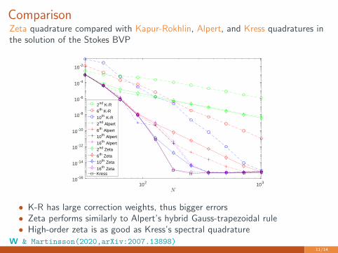
ComparisonZeta quadrature compared with Kapur-Rokhlin, Alpert, and Kress quadratures inthe solution of the Stokes BVP
102 10310-16
10-14
10-12
10-10
10-8
10-6
10-4
10-2
2nd K-R
6th K-R
10th K-R
2nd Alpert
6th Alpert
10th Alpert
16th Alpert
2nd Zeta
6th Zeta
10th Zeta
16th ZetaKress
• K-R has large correction weights, thus bigger errors• Zeta performs similarly to Alpert’s hybrid Gauss-trapezoidal rule• High-order zeta is as good as Kress’s spectral quadrature
W & Martinsson(2020,arXiv:2007.13898)11/14
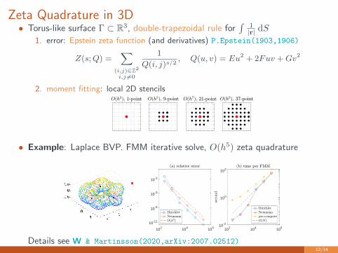
Zeta Quadrature in 3D• Torus-like surface Γ ⊂ R3, double-trapezoidal rule for
∫1|r| dS
1. error: Epstein zeta function (and derivatives) P.Epstein(1903,1906)
Z(s;Q) =∑
(i,j)∈Z2
i,j 6=0
1
Q(i, j)s/2, Q(u, v) = Eu2 + 2Fuv +Gv2
2. moment fitting: local 2D stencils
• Example: Laplace BVP. FMM iterative solve, O(h5) zeta quadrature
102 104 106
10-11
10-8
10-5
10-2
102 104 10610-2
100
102
Details see W & Martinsson(2020,arXiv:2007.02512)12/14
Historical Comments• I.Navot (J.Math.Phys.,1961 & 1962)
• extended Euler-Maclaurin formula for∫ 1
0x−sg(x) dx and
∫ 1
0g(x) log xdx
• A.Sidi,M.Israeli (J.Sci.Comput.,1988)
• high-order quadrature for∫ 1
0g(x) log x dx via extrapolation
• Celorrio,Sayas (BIT,1998)
• a proof for∫ 1/2
−1/2g(x) log x2 dx; mentioned Navot & ζ in the end.
• Kapur,Rokhlin (1997): another proof of the Navot(1962) result
• Marin,Runborg,Tornberg (2014)
• another proof of the Navot(1961) result; partial proof for∫
1|r| in R2.
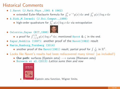
• Looks like Navot’s results had been rediscovered many times! (us included!)• Our path: surfaces (Epstein zeta) −→ curves (Riemann zeta)• Borwein et al.(2013) Lattice sums then and now
• Epstein zeta function, Wigner limits.
13/14
Conclusion
• Zeta functions are connected to trapezoidal quadrature errors
• Geometric analysis is the key to zeta quadratures on curves & surfaces
• Zeta quadratures are simple & robust, ideal for developing FDS
• Currently non-adaptive
• Codes available:
(2D) https://github.com/bobbielf2/ZetaTrap2D
(3D) https://github.com/bobbielf2/ZetaTrap3D
• More at the SIAM CSE21 conference
14/14

backup slides
15/14
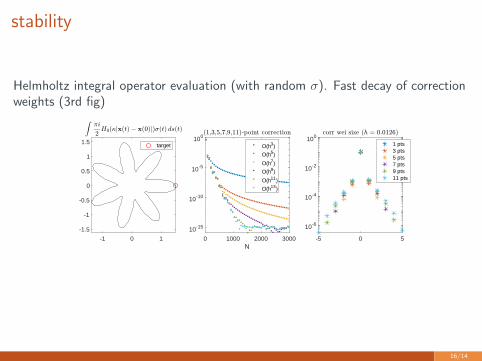
stability
Helmholtz integral operator evaluation (with random σ). Fast decay of correctionweights (3rd fig)
-5 0 5
10-6
10-4
10-2
100
1 pts3 pts5 pts7 pts9 pts11 pts
0 1000 2000 3000N
10-15
10-10
10-5
100
O(h3)
O(h5)
O(h7)
O(h9)
O(h11)
O(h13)
-1 0 1
-1.5
-1
-0.5
0
0.5
1
1.5 target
16/14
Top Related