


γλώσσες
Σελίδες
Νομικός

Programs to Calculate some Mathematical
Constants to Large Precision
Document Version 1.50
Prepared Using LATEX
by
Stefan Spannare
E-mail: [email protected]
September 19, 2007
1
Contents
1 Introduction
2 Disclaimer
3 General information
4 Some numerical values
5 Algorithms for π5.1 π, Borwein’s 4-th order5.2 π, Borwein’s 2-th order5.3 π, Gauss-Legendre, AGM5.4 π, Ramanujan series5.5 π, Chudnovsky series
6 Algorithms for ex = exp (x) and e = exp (1)6.1 ex = exp (x), Newton’s Iteration6.2 e = exp (1), using the series
∑
1/k!6.3 e = exp (1),
∑
1/k! using FEE
7 Algorithms for ln (x) and ln (2)7.1 ln (x), AGM7.2 ln (2), arctanh(x) based methods
8 Algorithms for Euler C, γ
9 Algorithms for Γ(1/3) and Γ(1/4)9.1 Γ(1/3)9.2 Γ(1/4)9.3 AGM
10 Algorithms for Catalan’s constant G
11 Algorithms for Apery’s constant ζ(3)
12 Algorithms for ζ(s)
13 Algorithms for inversion, division, square and cube roots13.1 Inversion 1/v and division13.2 1/
√v and
√v
13.3 1/v13 and v
13
13.4 1/v14 and v
14
14 Time complexity of algorithms
15 Accuracy and benchmarks15.1 Accuracy of calculations15.2 Benchmarks
16 References16.1 Book and article references16.2 Internet references
2
1 Introduction
Note, this document is under development. Please look back for updated versions.
This documents describes algorithms to calculate some mathematical constants used by some of the C-programs in the program package SSPROG. Some timings, benchmarks and references are also given.The programs are not so fast (much faster programs exist especially for π) but they demonstrates theprinciple of multi precision calculations. See also the header of each C-program source code for moreinformation.
At present algorithms used by the programs sspi, sseln2, ssgamma, ssgam134, sscatal, sszeta3,
sszeta and sspieln2 (in the NUMBERS directory) are described in this document.
The home page of the author and the web page of the program package and this document are foundhere:
http://www.spaennare.se/index.html
http://www.spaennare.se/ssprog.html
2 Disclaimer
For all the programs in this package the following statement is valid:
I make no warranties that this program is (1) free of errors, (2) consistent with any standard merchantabil-ity, or (3) meeting the requirements of a particular application. This software shall not, partly or as awhole, participate in a process, whose outcome can result in injury to a person or loss of property. Itis solely designed for analytical work. Permission to use, copy, and distribute is hereby granted withoutfee, providing that the header above including this notice appears in all copies.
Please report comments and bugs in both the programs and this document to:
E-mail: [email protected]
3 General information
The mathematical constants are calculated to desired precision (i.e. n decimal digits). Functions formulti precision calculations are included in the programs in this package. Especially fast FFT basedmultiplication must be used for large numbers. This presentation of the algorithms is quite brief (onlythe formulas). To put the constants in a wider context see for example reference [6]. This is the defaultreference throughout this document.
The natural logarithm is sometimes denoted log (x) and sometimes ln (x). The author prefers ln (x) whichis used in this document.
A comment regarding the FEE (Fast E-function Evaluation) method for very fast evaluation of transcen-dental functions (series). The method was invented 1991 by Ekatherina A. Karatsuba, Russia. Anothermethod called ”divide and conquer” was invented earlier by Anatoly Karatsuba. This method was thencalled ”binary splitting” by some people. However, by later years it seems as if ”binary splitting” hasbeen erroneously taken as a name also for the FEE method by some people preferably in the westerncountries. The correct name FEE is used throughout this document. See also references [1], [7] and [8].
3
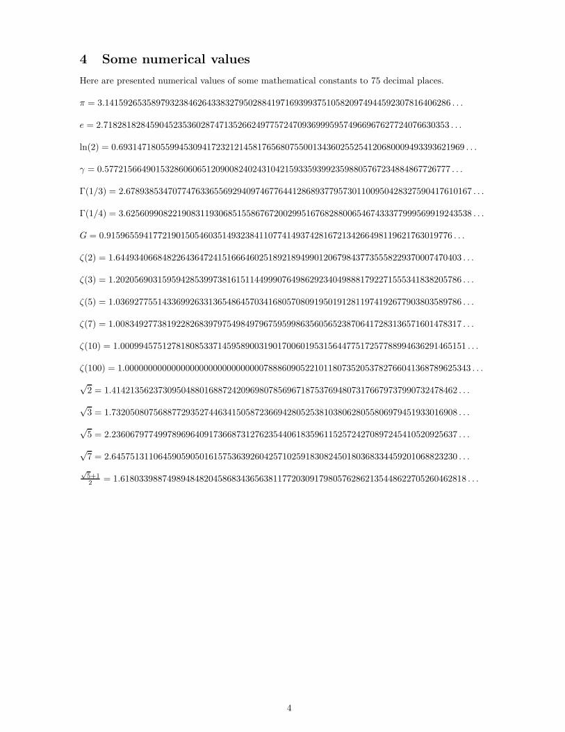
4 Some numerical values
Here are presented numerical values of some mathematical constants to 75 decimal places.
π = 3.141592653589793238462643383279502884197169399375105820974944592307816406286 . . .
e = 2.718281828459045235360287471352662497757247093699959574966967627724076630353 . . .
ln(2) = 0.693147180559945309417232121458176568075500134360255254120680009493393621969 . . .
γ = 0.577215664901532860606512090082402431042159335939923598805767234884867726777 . . .
Γ(1/3) = 2.678938534707747633655692940974677644128689377957301100950428327590417610167 . . .
Γ(1/4) = 3.625609908221908311930685155867672002995167682880065467433377999569919243538 . . .
G = 0.915965594177219015054603514932384110774149374281672134266498119621763019776 . . .
ζ(2) = 1.644934066848226436472415166646025189218949901206798437735558229370007470403 . . .
ζ(3) = 1.202056903159594285399738161511449990764986292340498881792271555341838205786 . . .
ζ(5) = 1.036927755143369926331365486457034168057080919501912811974192677903803589786 . . .
ζ(7) = 1.008349277381922826839797549849796759599863560565238706417283136571601478317 . . .
ζ(10) = 1.000994575127818085337145958900319017006019531564477517257788994636291465151 . . .
ζ(100) = 1.000000000000000000000000000000788860905221011807352053782766041368789625343 . . .
√2 = 1.414213562373095048801688724209698078569671875376948073176679737990732478462 . . .
√3 = 1.732050807568877293527446341505872366942805253810380628055806979451933016908 . . .
√5 = 2.236067977499789696409173668731276235440618359611525724270897245410520925637 . . .
√7 = 2.645751311064590590501615753639260425710259183082450180368334459201068823230 . . .
√5+1
2= 1.618033988749894848204586834365638117720309179805762862135448622705260462818 . . .
4
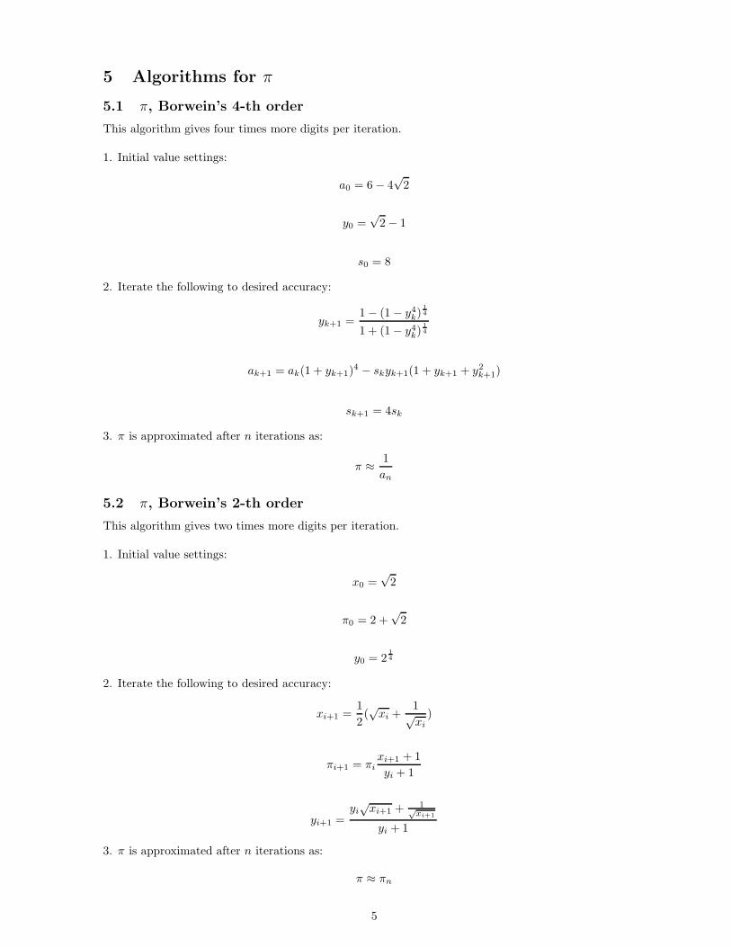
5 Algorithms for π
5.1 π, Borwein’s 4-th order
This algorithm gives four times more digits per iteration.
1. Initial value settings:
a0 = 6 − 4√
2
y0 =√
2 − 1
s0 = 8
2. Iterate the following to desired accuracy:
yk+1 =1 − (1 − y4
k)14
1 + (1 − y4k)
14
ak+1 = ak(1 + yk+1)4 − skyk+1(1 + yk+1 + y2
k+1)
sk+1 = 4sk
3. π is approximated after n iterations as:
π ≈1
an
5.2 π, Borwein’s 2-th order
This algorithm gives two times more digits per iteration.
1. Initial value settings:
x0 =√
2
π0 = 2 +√
2
y0 = 214
2. Iterate the following to desired accuracy:
xi+1 =1
2(√
xi +1
√xi
)
πi+1 = πixi+1 + 1
yi + 1
yi+1 =yi√
xi+1 + 1√xi+1
yi + 1
3. π is approximated after n iterations as:
π ≈ πn
5
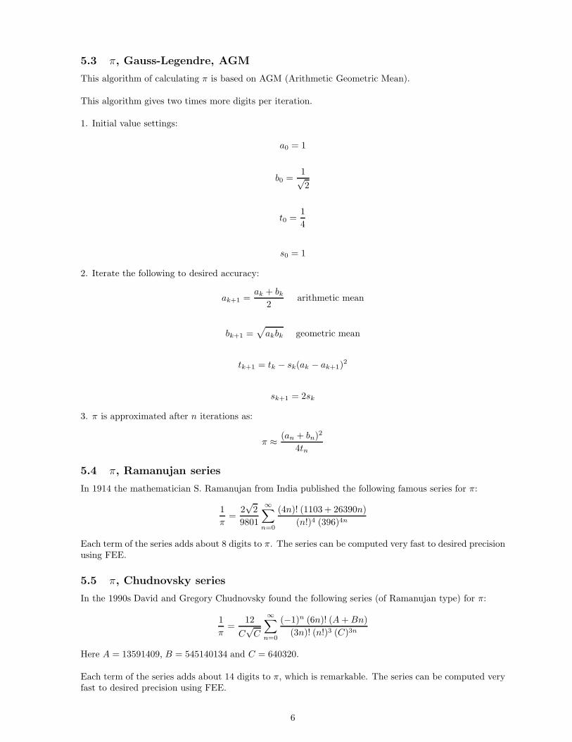
5.3 π, Gauss-Legendre, AGM
This algorithm of calculating π is based on AGM (Arithmetic Geometric Mean).
This algorithm gives two times more digits per iteration.
1. Initial value settings:
a0 = 1
b0 =1√
2
t0 =1
4
s0 = 1
2. Iterate the following to desired accuracy:
ak+1 =ak + bk
2arithmetic mean
bk+1 =√
akbk geometric mean
tk+1 = tk − sk(ak − ak+1)2
sk+1 = 2sk
3. π is approximated after n iterations as:
π ≈(an + bn)2
4tn
5.4 π, Ramanujan series
In 1914 the mathematician S. Ramanujan from India published the following famous series for π:
1
π=
2√
2
9801
∞∑
n=0
(4n)! (1103 + 26390n)
(n!)4 (396)4n
Each term of the series adds about 8 digits to π. The series can be computed very fast to desired precisionusing FEE.
5.5 π, Chudnovsky series
In the 1990s David and Gregory Chudnovsky found the following series (of Ramanujan type) for π:
1
π=
12
C√
C
∞∑
n=0
(−1)n (6n)! (A + Bn)
(3n)! (n!)3 (C)3n
Here A = 13591409, B = 545140134 and C = 640320.
Each term of the series adds about 14 digits to π, which is remarkable. The series can be computed veryfast to desired precision using FEE.
6
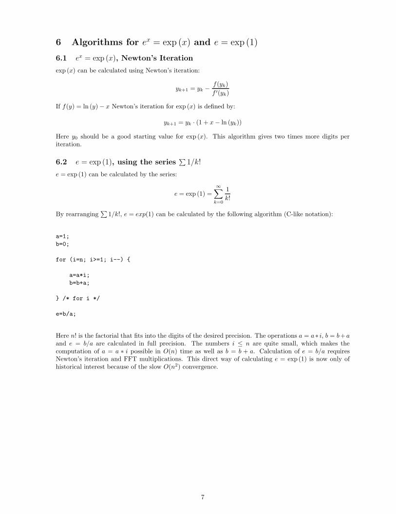
6 Algorithms for ex = exp (x) and e = exp (1)
6.1 ex = exp (x), Newton’s Iteration
exp (x) can be calculated using Newton’s iteration:
yk+1 = yk −f(yk)
f ′(yk)
If f(y) = ln (y) − x Newton’s iteration for exp (x) is defined by:
yk+1 = yk · (1 + x − ln (yk))
Here y0 should be a good starting value for exp (x). This algorithm gives two times more digits periteration.
6.2 e = exp (1), using the series∑
1/k!
e = exp (1) can be calculated by the series:
e = exp (1) =
∞∑
k=0
1
k!
By rearranging∑
1/k!, e = exp(1) can be calculated by the following algorithm (C-like notation):
a=1;
b=0;
for (i=n; i>=1; i--) {
a=a*i;
b=b+a;
} /* for i */
e=b/a;
Here n! is the factorial that fits into the digits of the desired precision. The operations a = a∗ i, b = b+aand e = b/a are calculated in full precision. The numbers i ≤ n are quite small, which makes thecomputation of a = a ∗ i possible in O(n) time as well as b = b + a. Calculation of e = b/a requiresNewton’s iteration and FFT multiplications. This direct way of calculating e = exp (1) is now only ofhistorical interest because of the slow O(n2) convergence.
7
6.3 e = exp (1),∑
1/k! using FEE
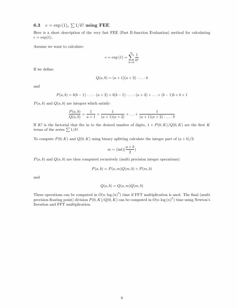
Here is a short description of the very fast FEE (Fast E-function Evaluation) method for calculatinge = exp(1).
Assume we want to calculate:
e = exp (1) =
∞∑
k=0
1
k!
If we define:
Q(a, b) = (a + 1)(a + 2) · . . . · b
and
P (a, b) = b(b − 1) · . . . · (a + 2) + b(b − 1) · . . . · (a + 3) + . . . + (b − 1)b + b + 1
P (a, b) and Q(a, b) are integers which satisfy:
P (a, b)
Q(a, b)=
1
a + 1+
1
(a + 1)(a + 2)+ . . . +
1
(a + 1)(a + 2) · . . . · b
If K! is the factorial that fits in to the desired number of digits, 1 + P (0, K)/Q(0, K) are the first Kterms of the series
∑
1/k!.
To compute P (0, K) and Q(0, K) using binary splitting calculate the integer part of (a + b)/2:
m = (int)(a + b
2)
P (a, b) and Q(a, b) are then computed recursively (multi precision integer operations):
P (a, b) = P (a, m)Q(m, b) + P (m, b)
and
Q(a, b) = Q(a, m)Q(m, b)
These operations can be computed in O(n log (n)3) time if FFT multiplication is used. The final (multi
precision floating point) division P (0, K)/Q(0, K) can be computed in O(n log (n)2) time using Newton’s
Iteration and FFT multiplication.
8
7 Algorithms for ln (x) and ln (2)
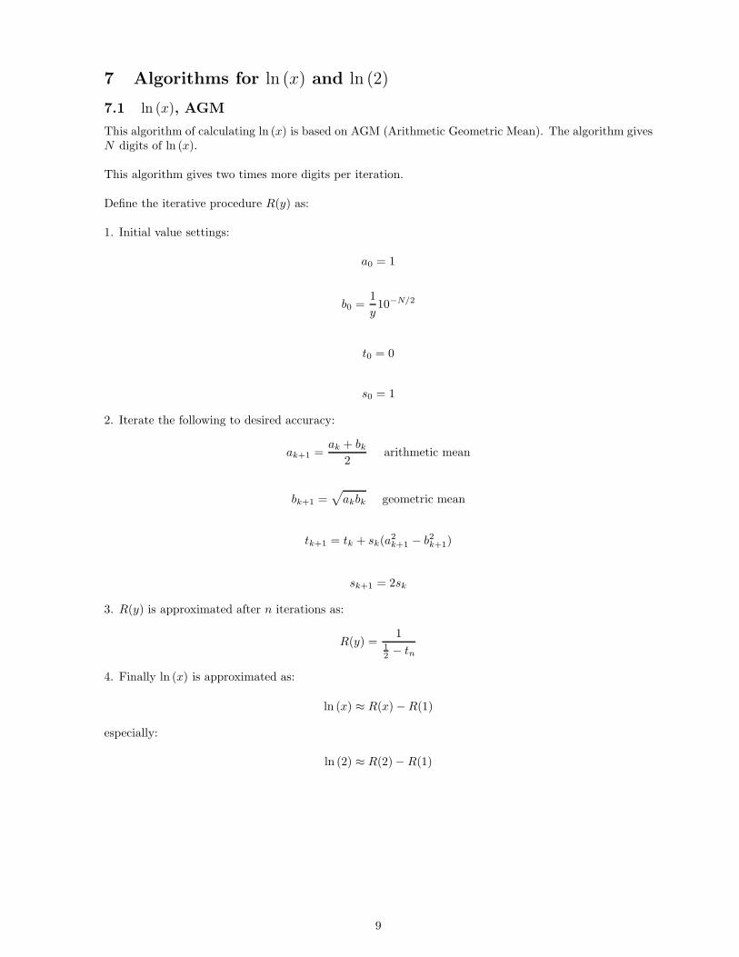
7.1 ln (x), AGM
This algorithm of calculating ln (x) is based on AGM (Arithmetic Geometric Mean). The algorithm givesN digits of ln (x).
This algorithm gives two times more digits per iteration.
Define the iterative procedure R(y) as:
1. Initial value settings:
a0 = 1
b0 =1
y10−N/2
t0 = 0
s0 = 1
2. Iterate the following to desired accuracy:
ak+1 =ak + bk
2arithmetic mean
bk+1 =√
akbk geometric mean
tk+1 = tk + sk(a2k+1 − b2
k+1)
sk+1 = 2sk
3. R(y) is approximated after n iterations as:
R(y) =1
1
2− tn
4. Finally ln (x) is approximated as:
ln (x) ≈ R(x) − R(1)
especially:
ln (2) ≈ R(2) − R(1)
9
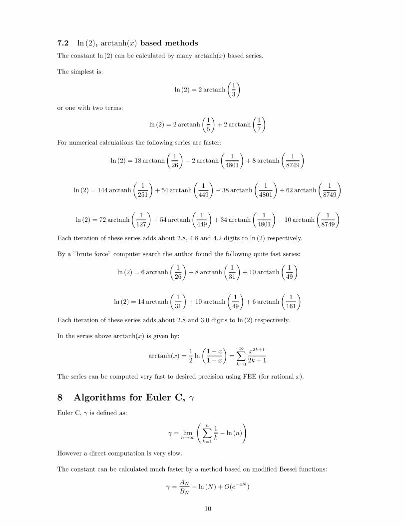
7.2 ln (2), arctanh(x) based methods
The constant ln (2) can be calculated by many arctanh(x) based series.
The simplest is:
ln (2) = 2 arctanh
(
1
3
)
or one with two terms:
ln (2) = 2 arctanh
(
1
5
)
+ 2 arctanh
(
1
7
)
For numerical calculations the following series are faster:
ln (2) = 18 arctanh
(
1
26
)
− 2 arctanh
(
1
4801
)
+ 8 arctanh
(
1
8749
)
ln (2) = 144 arctanh
(
1
251
)
+ 54 arctanh
(
1
449
)
− 38 arctanh
(
1
4801
)
+ 62 arctanh
(
1
8749
)
ln (2) = 72 arctanh
(
1
127
)
+ 54 arctanh
(
1
449
)
+ 34 arctanh
(
1
4801
)
− 10 arctanh
(
1
8749
)
Each iteration of these series adds about 2.8, 4.8 and 4.2 digits to ln (2) respectively.
By a ”brute force” computer search the author found the following quite fast series:
ln (2) = 6 arctanh
(
1
26
)
+ 8 arctanh
(
1
31
)
+ 10 arctanh
(
1
49
)
ln (2) = 14 arctanh
(
1
31
)
+ 10 arctanh
(
1
49
)
+ 6 arctanh
(
1
161
)
Each iteration of these series adds about 2.8 and 3.0 digits to ln (2) respectively.
In the series above arctanh(x) is given by:
arctanh(x) =1
2ln
(
1 + x
1 − x
)
=
∞∑
k=0
x2k+1
2k + 1
The series can be computed very fast to desired precision using FEE (for rational x).
8 Algorithms for Euler C, γ
Euler C, γ is defined as:
γ = limn→∞
(
n∑
k=1
1
k− ln (n)
)
However a direct computation is very slow.
The constant can be calculated much faster by a method based on modified Bessel functions:
γ =AN
BN− ln (N) + O(e−4N )
10
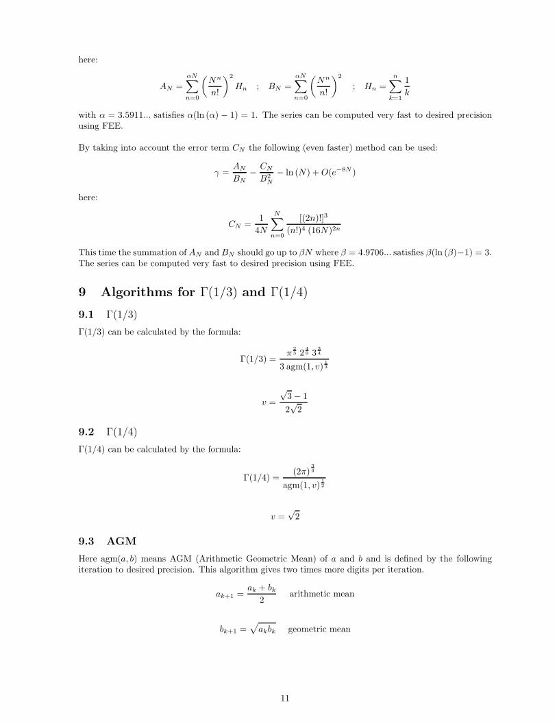
here:
AN =αN∑
n=0
(
Nn
n!
)2
Hn ; BN =αN∑
n=0
(
Nn
n!
)2
; Hn =n∑
k=1
1
k
with α = 3.5911... satisfies α(ln (α) − 1) = 1. The series can be computed very fast to desired precisionusing FEE.
By taking into account the error term CN the following (even faster) method can be used:
γ =AN
BN−
CN
B2N
− ln (N) + O(e−8N )
here:
CN =1
4N
N∑
n=0
[(2n)!]3
(n!)4 (16N)2n
This time the summation of AN and BN should go up to βN where β = 4.9706... satisfies β(ln (β)−1) = 3.The series can be computed very fast to desired precision using FEE.
9 Algorithms for Γ(1/3) and Γ(1/4)
9.1 Γ(1/3)
Γ(1/3) can be calculated by the formula:
Γ(1/3) =π
23 2
49 3
34
3 agm(1, v)13
v =
√3 − 1
2√
2
9.2 Γ(1/4)
Γ(1/4) can be calculated by the formula:
Γ(1/4) =(2π)
34
agm(1, v)12
v =√
2
9.3 AGM
Here agm(a, b) means AGM (Arithmetic Geometric Mean) of a and b and is defined by the followingiteration to desired precision. This algorithm gives two times more digits per iteration.
ak+1 =ak + bk
2arithmetic mean
bk+1 =√
akbk geometric mean
11
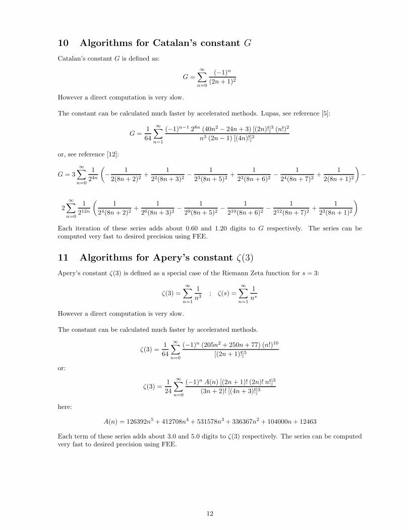
10 Algorithms for Catalan’s constant G
Catalan’s constant G is defined as:
G =∞∑
n=0
(−1)n
(2n + 1)2
However a direct computation is very slow.
The constant can be calculated much faster by accelerated methods. Lupas, see reference [5]:
G =1
64
∞∑
n=1
(−1)n−1 28n (40n2 − 24n + 3) [(2n)!]3 (n!)2
n3 (2n − 1) [(4n)!]2
or, see reference [12]:
G = 3
∞∑
n=0
1
24n
(
−1
2(8n + 2)2+
1
22(8n + 3)2−
1
23(8n + 5)2+
1
23(8n + 6)2−
1
24(8n + 7)2+
1
2(8n + 1)2
)
−
2
∞∑
n=0
1
212n
(
1
24(8n + 2)2+
1
26(8n + 3)2−
1
29(8n + 5)2−
1
210(8n + 6)2−
1
212(8n + 7)2+
1
23(8n + 1)2
)
Each iteration of these series adds about 0.60 and 1.20 digits to G respectively. The series can becomputed very fast to desired precision using FEE.
11 Algorithms for Apery’s constant ζ(3)
Apery’s constant ζ(3) is defined as a special case of the Riemann Zeta function for s = 3:
ζ(3) =∞∑
n=1
1
n3; ζ(s) =
∞∑
n=1
1
ns
However a direct computation is very slow.
The constant can be calculated much faster by accelerated methods.
ζ(3) =1
64
∞∑
n=0
(−1)n (205n2 + 250n + 77) (n!)10
[(2n + 1)!]5
or:
ζ(3) =1
24
∞∑
n=0
(−1)n A(n) [(2n + 1)! (2n)! n!]3
(3n + 2)! [(4n + 3)!]3
here:
A(n) = 126392n5 + 412708n4 + 531578n3 + 336367n2 + 104000n + 12463
Each term of these series adds about 3.0 and 5.0 digits to ζ(3) respectively. The series can be computedvery fast to desired precision using FEE.
12
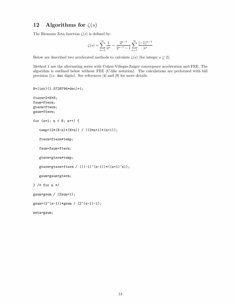
12 Algorithms for ζ(s)
The Riemann Zeta function ζ(s) is defined by:
ζ(s) =
∞∑
n=1
1
ns=
2s−1
2s−1 − 1
∞∑
n=1
(−1)n−1
ns
Below are described two accelerated methods to calculate ζ(s) (for integer s ≥ 2).
Method 1 use the alternating series with Cohen-Villegas-Zaiger convergence acceleration and FEE. Thealgorithm is outlined below without FEE (C-like notation). The calculations are performed with fullprecision (i.e. dec digits). See references [4] and [9] for more details.
N=(int)(1.5728794*dec)+1;
fterm=2*N*N;
fsum=fterm;
gterm=fterm;
gsum=fterm;
for (n=1; n < N; n++) {
temp=(2*(N-n)*(N+n)) / ((2*n+1)*(n+1));
fterm=fterm*temp;
fsum=fsum+fterm;
gterm=gterm*temp;
gterm=gterm+fterm / (((-1)^(n-1))*((n+1)^s));
gsum=gsum+gterm;
} /* for n */
gsum=gsum / (fsum+1);
gsum=(2^(s-1))*gsum / (2^(s-1)-1);
zeta=gsum;
13
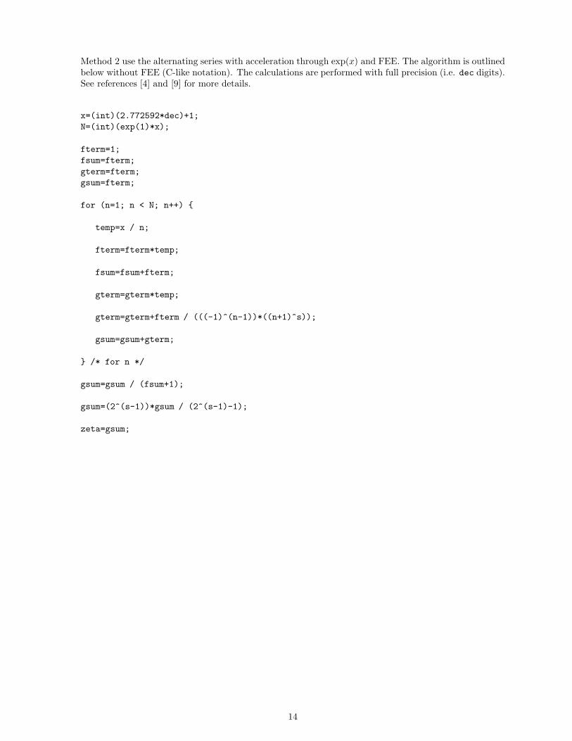
Method 2 use the alternating series with acceleration through exp(x) and FEE. The algorithm is outlinedbelow without FEE (C-like notation). The calculations are performed with full precision (i.e. dec digits).See references [4] and [9] for more details.
x=(int)(2.772592*dec)+1;
N=(int)(exp(1)*x);
fterm=1;
fsum=fterm;
gterm=fterm;
gsum=fterm;
for (n=1; n < N; n++) {
temp=x / n;
fterm=fterm*temp;
fsum=fsum+fterm;
gterm=gterm*temp;
gterm=gterm+fterm / (((-1)^(n-1))*((n+1)^s));
gsum=gsum+gterm;
} /* for n */
gsum=gsum / (fsum+1);
gsum=(2^(s-1))*gsum / (2^(s-1)-1);
zeta=gsum;
14
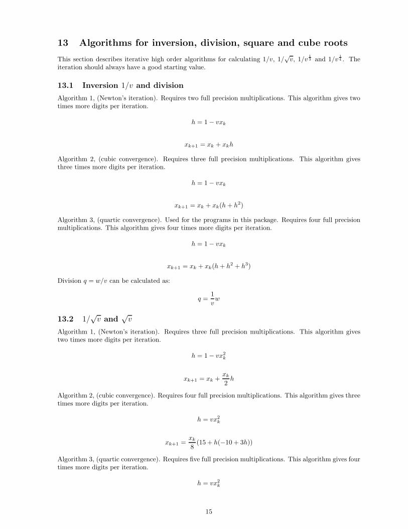
13 Algorithms for inversion, division, square and cube roots
This section describes iterative high order algorithms for calculating 1/v, 1/√
v, 1/v13 and 1/v
14 . The
iteration should always have a good starting value.
13.1 Inversion 1/v and division
Algorithm 1, (Newton’s iteration). Requires two full precision multiplications. This algorithm gives twotimes more digits per iteration.
h = 1 − vxk
xk+1 = xk + xkh
Algorithm 2, (cubic convergence). Requires three full precision multiplications. This algorithm givesthree times more digits per iteration.
h = 1 − vxk
xk+1 = xk + xk(h + h2)
Algorithm 3, (quartic convergence). Used for the programs in this package. Requires four full precisionmultiplications. This algorithm gives four times more digits per iteration.
h = 1 − vxk
xk+1 = xk + xk(h + h2 + h3)
Division q = w/v can be calculated as:
q =1
vw
13.2 1/√
v and√
v
Algorithm 1, (Newton’s iteration). Requires three full precision multiplications. This algorithm givestwo times more digits per iteration.
h = 1 − vx2k
xk+1 = xk +xk
2h
Algorithm 2, (cubic convergence). Requires four full precision multiplications. This algorithm gives threetimes more digits per iteration.
h = vx2k
xk+1 =xk
8(15 + h(−10 + 3h))
Algorithm 3, (quartic convergence). Requires five full precision multiplications. This algorithm gives fourtimes more digits per iteration.
h = vx2k
15
xk+1 =xk
16(35 + h(−35 + h(21 − 5h)))
A more efficient way to write this is (used for the programs in this package):
h = 1 − vx2k
xk+1 = xk +xk
16(8h + 6h2 + 5h3)
√v can then be calculated as:
√v ≈ vxn
13.3 1/v1
3 and v1
3
Algorithm 1, (Newton’s iteration). Requires four full precision multiplications. This algorithm gives twotimes more digits per iteration.
h = 1 − vx3k
xk+1 = xk +xk
3h
Algorithm 2, (quartic convergence). Used for for the programs in this package. Requires six full precisionmultiplications. This algorithm gives four times more digits per iteration.
h = 1 − vx3k
xk+1 = xk +xk
162(54h + 36h2 + 28h3)
v13 can then be calculated as:
v13 ≈ vx2
n
13.4 1/v1
4 and v1
4
Algorithm 1, (Newton’s iteration). Requires four full precision multiplications. This algorithm gives twotimes more digits per iteration.
h = 1 − vx4k
xk+1 = xk +xk
4h
Algorithm 2, (quartic convergence). Requires six full precision multiplications. This algorithm gives fourtimes more digits per iteration.
h = vx4k
xk+1 =xk
128(195 + h(−117 + h(65 − 15h)))
A more efficient way to write this is (used for the programs in this package):
h = 1 − vx4k
xk+1 = xk +xk
128(32h + 20h2 + 15h3)
v14 can then be calculated as:
v14 ≈ vx3
n
16
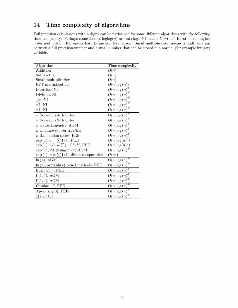
14 Time complexity of algorithms
Full precision calculations with n digits can be performed for some different algorithms with the followingtime complexity. Perhaps some factors loglog(n) are missing. NI means Newton’s Iteration (or higherorder methods). FEE means Fast E-function Evaluation. Small multiplication means a multiplicationbetween a full precision number and a small number that can be stored in a normal (for example integer)variable.
Algorithm Time complexityAddition O(n)Subtraction O(n)Small multiplication O(n)FFT multiplication O(n log (n))
Inversion, NI O(n log (n)2)
Division, NI O(n log (n)2)√
x, NI O(n log (n)2)
x13 , NI O(n log (n)2)
x14 , NI O(n log (n)2)
π Borwein’s 4-th order O(n log (n)3)
π Borwein’s 2-th order O(n log (n)3)
π Gauss Legendre, AGM O(n log (n)3)
π Chudnovsky series, FEE O(n log (n)3)
π Ramanujan series, FEE O(n log (n)3)
exp (1), e =∑
1/k!, FEE O(n log(n)3)exp (1), 1/e =
∑
(−1)k/k!, FEE O(n log(n)3)
exp (x), NI (using ln (x) AGM) O(n log (n)4)
exp (1), e =∑
1/k!, direct computation O(n2)
ln (x), AGM O(n log (n)3)
ln (2), arctanh(x) based methods, FEE O(n log (n)3)
Euler C, γ, FEE O(n log (n)3)
Γ(1/3), AGM O(n log (n)3)
Γ(1/4), AGM O(n log (n)3)
Catalan, G, FEE O(n log (n)3)
Apery’s, ζ(3), FEE O(n log (n)3)
ζ(s), FEE O(n log (n)3)
17
15 Accuracy and benchmarks
15.1 Accuracy of calculations
The programs in this package calculate the mathematical constants below to many decimal places. Allprinted digits are supposed to be correct. The programs use a very fast FFT (fftsg h.c) by Takuya Ooura(see reference [10]).
Warning! If you want to calculate more than 224 (about 16 million) digits set the constant mulversion= 2 in the file ”mulver.txt” to avoid errors in the FFT multiplication. At least this must be done if ”FFTmax error” > 0.25. This makes the programs two times slower and requires more memory.
15.2 Benchmarks
Some other good web-pages about benchmarks of mathematical constants are found in references [13]and [14].
In these benchmarks the FFT multiplication variable (mulversion) was set to 1 (i.e. fastest method).
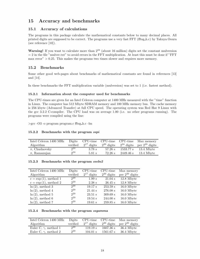
15.2.1 Information about the computer used for benchmarks
The CPU-times are given for an Intel Celeron computer at 1400 MHz measured with the ”time” functionin Linux. The computer has 512 Mbyte SDRAM memory and 100 MHz memory bus. The cache memoryis 256 kbyte (Advanced Transfer) at full CPU speed. The operating system was Red Hat 9 Linux withthe gcc 3.2.2 C-compiler. The CPU load was on average 1.00 (i.e. no other programs running). Theprograms were compiled using the line:
>gcc -O3 -o program program.c fftsg h.c -lm
15.2.2 Benchmarks with the program sspi
Intel Celeron 1400 MHz Digits CPU-time CPU-time CPU-time Max memoryAlgorithm verified 217 digits 220 digits 224 digits per 220 digitsπ, Chudnovsky 224 3.78 s 57.26 s 1533.77 s 13.4 Mbyteπ, Ramanujan 224 5.81 s 72.26 s 2449.46 s 13.4 Mbyte
15.2.3 Benchmarks with the program sseln2
Intel Celeron 1400 MHz Digits CPU-time CPU-time Max memoryAlgorithm verified 217 digits 220 digits per 220 digitse = exp (1), method 1 220 1.99 s 21.04 s 12.8 Mbytee = exp (1), method 2 220 2.38 s 26.45 s 12.8 Mbyteln (2), method 3 220 19.17 s 253.59 s 16.0 Mbyteln (2), method 4 220 21.44 s 276.08 s 16.0 Mbyteln (2), method 5 220 23.51 s 309.69 s 16.0 Mbyteln (2), method 6 220 19.54 s 244.00 s 16.0 Mbyteln (2), method 7 220 19.61 s 259.85 s 16.0 Mbyte
15.2.4 Benchmarks with the program ssgamma
Intel Celeron 1400 MHz Digits CPU-time CPU-time Max memoryAlgorithm verified 217 digits 220 digits per 220 digitsEuler C, γ, method 1 220 119.19 s 1607.36 s 36.4 MbyteEuler C, γ, method 2 220 104.01 s 1561.67 s 36.4 Mbyte
18
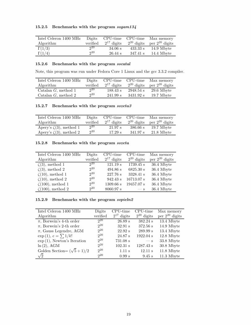
15.2.5 Benchmarks with the program ssgam134
Intel Celeron 1400 MHz Digits CPU-time CPU-time Max memoryAlgorithm verified 217 digits 220 digits per 220 digitsΓ(1/3) 220 34.06 s 433.33 s 14.9 MbyteΓ(1/4) 220 26.44 s 347.41 s 14.4 Mbyte
15.2.6 Benchmarks with the program sscatal
Note, this program was run under Fedora Core 1 Linux and the gcc 3.3.2 compiler.
Intel Celeron 1400 MHz Digits CPU-time CPU-time Max memoryAlgorithm verified 217 digits 220 digits per 220 digitsCatalan G, method 1 220 188.43 s 2948.54 s 29.6 MbyteCatalan G, method 2 220 241.99 s 3431.92 s 19.7 Mbyte
15.2.7 Benchmarks with the program sszeta3
Intel Celeron 1400 MHz Digits CPU-time CPU-time Max memoryAlgorithm verified 217 digits 220 digits per 220 digitsApery’s ζ(3), method 1 220 21.97 s 386.66 s 19.7 MbyteApery’s ζ(3), method 2 220 17.29 s 341.97 s 21.8 Mbyte
15.2.8 Benchmarks with the program sszeta
Intel Celeron 1400 MHz Digits CPU-time CPU-time Max memoryAlgorithm verified 217 digits 220 digits per 220 digitsζ(3), method 1 220 121.19 s 1739.45 s 36.4 Mbyteζ(3), method 2 220 494.86 s 6825.30 s 36.4 Mbyteζ(10), method 1 220 227.76 s 3328.41 s 36.4 Mbyteζ(10), method 2 220 942.43 s 16713.07 s 36.4 Mbyteζ(100), method 1 220 1309.66 s 19457.07 s 36.4 Mbyteζ(100), method 2 220 8060.97 s — s 36.4 Mbyte
15.2.9 Benchmarks with the program sspieln2
Intel Celeron 1400 MHz Digits CPU-time CPU-time Max memoryAlgorithm verified 217 digits 220 digits per 220 digitsπ, Borwein’s 4-th order 220 26.89 s 382.24 s 13.4 Mbyteπ, Borwein’s 2-th order 220 32.91 s 372.56 s 14.9 Mbyteπ, Gauss Legendre, AGM 220 22.92 s 289.99 s 13.4 Mbyteexp (1), e =
∑
1/k! 220 24.87 s 1922.04 s 12.8 Mbyteexp (1), Newton’s Iteration 220 731.08 s — s 33.8 Mbyteln (2), AGM 220 102.31 s 1287.43 s 30.8 Mbyte
Golden Section= (√
5 + 1)/2 220 1.11 s 12.11 s 11.8 Mbyte√2 220 0.99 s 9.45 s 11.3 Mbyte
19
16 References
16.1 Book and article references
[1] Ekatherina A. Karatsuba, ”Fast evaluation of transcendental functions”, Problems of Information
Transmission, vol. 27, (1991), p. 339-360.
[2] ”Pi and the AGM, A Study in Analytic Number Theory and Computational Complexity”, Volume 4,by Jonathan M. Borwein and Peter B. Borwein, 1987. A Wiley-Interscience Publication, JOHN WILEY& SON INC.
[3] ”Fast multiprecision evaluation of series of rational numbers”, by Bruno Haible and Thomas Pa-panikolaou, 1997.
[4] ”Convergence Acceleration of Alternating Series”, by H. Cohen, F. R. Villegas and D. Zaiger, Bonn,(1991).
[5] ”Formulae for some classical constants”, (to appear in Proceedings of ROGER-2000), by AlexandruLupas.
16.2 Internet references
The iterative (high order) formulas for calculating 1/√
v and 1/v14 and the rearranged method to calculate
e = exp (1) =∑
1/k! were derived by the author of this document. The home page of the author andthe web page of the program package and this document are found here:
http://www.spaennare.se/index.html
http://www.spaennare.se/ssprog.html
Most other information is found on Internet. Many people are calculating different mathematical con-stants (mostly π) to many decimal places just for fun or scientific purposes. Different algorithms forcalculating the constants can be found on many places on Internet.
[6] ”Mathematical constants and computation”, by Xavier Gourdon and Pascal Sebah. Here is describedalmost everything you want to know about mathematical constants and how to compute them. One ofthe fastest programs for calculating π and other constants on a PC is also found here.
http://numbers.computation.free.fr/Constants/constants.html
[7] ”Fast Algorithms and the FEE Method”, by Ekatherina A. Karatsuba.
http://www.ccas.ru/personal/karatsuba/algen.htm
[8] ”The Karatsuba Method ’Divide and Conquer’”, by Ekatherina A. Karatsuba.
http://www.ccas.ru/personal/karatsuba/divcen.htm
[9] ”CLN - Class Library for Numbers”, by Bruno Haible et. al.
http://www.ginac.de/CLN/
20
[10] ”Ooura’s Mathematical Software Packages”, by Takuya Ooura. Among other things many fast FFTswritten in C and Fortran.
http://www.kurims.kyoto-u.ac.jp/∼ooura/
[11] ”Plouffe’s Inverter”, by Simon Plouffe. Some interesting digit records. Files containing differentnumbers to many decimal places can also be found here. These files can be used for verification purposes.
http://pi.lacim.uqam.ca/eng/
[12] ”The Wolfram Functions Site”. Created with Mathematica by Wolfram Research. Very goodinformation about mathematics.
http://functions.wolfram.com
[13] ”Dara’s π Pages”. Comparison of different π calculating programs etc.
http://www.myownlittleworld.com/miscellaneous/computers/pilargetable.html
[14] ”Stu’s Pi page”. Record page for the fastest π programs for PC. The record holder can also bedownloaded here.
http://home.istar.ca/∼lyster/pi.html
21
Top Related