


γλώσσες
Σελίδες
Νομικός

PROBABILITY AND STATISTICAL INFERENCE
Probability vs. Statistics – Standard Viewpoint:
“Probability” postulates a probability model and uses this to predict thebehavior of observed data.
“Statistics” uses observed data to infer the probability model (= distribu-tion) from which the data was generated.
1. Probability Distributions and Random Variables.
1.1. The components (Ω,S, P ) of a probability model (≡ randomexperiment):
Ω := sample space = set of all possible outcomes of the random experiment.
Ω either discrete (finite or countable) or continuous (≈ open subset of Rn).
Example 1.1. Toss a coin n times: Ω = all sequences HHTH . . . TH oflength n (H = Heads, T = Tails). Thus |Ω| = 2n (finite), so Ω is discrete.
Example 1.2. Toss a coin repeatedly until Heads appears and record thenumber of tosses needed: Ω = 1, 2, . . . (countable) so Ω is again discrete.
Example 1.3. Spin a pointer and record the angle where the pointer comesto rest: Ω = [0, 2π) ⊂ R1, an entire interval, so Ω is continuous.
Example 1.4. Toss a dart at a circular board of radius d and recordthe impact point: Ω = (x, y) | x2 + y2 ≤ d2 ⊂ R2, a solid disk; Ω iscontinuous.
Example 1.5. Toss a coin infinitely many times: Ω = all infinite sequencesHHTH . . .. Here Ω 1−1←→ [0, 1] ⊂ R1 [why?], so Ω is continuous.
Example 1.6. (Brownian motion) Observe the path of a particle sus-pended in a liquid or gaseous medium: Ω is the set of all continuous paths(functions), so Ω is continuous but not finite-dimensional.
Note: Examples 1.5 and 1.6 are examples of discrete-time and continuous-time stochastic processes, respectively.
1
S := class of (measurable) events A ⊆ Ω.
We assume that S is a σ-field ( ≡ σ-algebra), that is:
(a) ∅,Ω ∈ S;
(b) A ∈ S ⇒ Ac ∈ S;
(c) Ai ⊆ S ⇒ ∪∞i=1Ai ∈ S.
In the discrete case, S = 2Ω = all possible subsets of Ω is a σ-field.
In the continuous case, usually S = Bn(Ω), the Borel σ-field generated byall open subsets of Ω. (Write Bn for Bn(Rn).)
(For stochastic processes, must define B∞ carefully.)
P := a probability measure: P (A) = probability that A occurs. Require:
(a) 0 ≤ P (A) ≤ 1;
(b) P (∅) = 0, P (Ω) = 1.
(c) Ai ⊆ S, disjoint, ⇒ P (∪∞i=1Ai) =
∑∞i=1 P (Ai). (count’le additivity)
(c) ⇒ P (Ac) = 1 − P (A).
In the discrete case where Ω = ω1, ω2, . . ., P is completely determinedby the elementary probabilities pk ≡ P (ωk), k = 1, 2, . . .. This is becausecountable additivity implies that
(1.1) P (A) =∑ω∈A
P (ω) ∀ A ∈ S ≡ 2Ω.
Conversely, given any set of numbers p1, p2, . . . that satisfy
(a) pk ≥ 0,
(b)∑∞
k=1 pk = 1,
we can define a probability measure P on 2Ω via (1.1) [verify countableadditivity.] Here, p1, p2, . . . is called a probability mass function (pmf).
Example 1.7. The following pk are pmfs [verify (a) and (b)]:(n
k
)pk(1 − p)n−k, k = 0, 1, . . . , n (0 < p < 1) [Binomial(n, p)];(1.2)
(1 − p)k−1p, k = 1, 2, . . . (0 < p < 1) [Geometric(p)];(1.3)e−λλk/k!, k = 0, 1, . . . (λ > 0) [Poisson(λ)].(1.4)
2
The binomial distribution occurs in Example 1.1; the geometric distributionoccurs in Example 1.2; the Poisson distribution arises as the limit of thebinomial distributions Bin(n, p) when n → ∞ and p → 0 such that np → λ;[Discuss details].
In the continuous case where (Ω,S) = (Rn,Bn), let f(·) be a (Borel-measurable) function on Rn that satisfies
(a) f(x1, . . . , xn) ≥ 0 ∀(x1, . . . , xn) ∈ Rn,
(b)∫
. . .∫
Rnf(x1, . . . , xn) dx1 . . . dxn = 1.
Then f(·) defines a probability measure P on (Rn,Bn) by
(1.5) P (B) =∫
. . .
∫B
f(x1, . . . , xn) dx1 . . . dxn ∀B ∈ Bn.
The function f(·) is called a probability density function (pdf) on Rn. Notethat in the continuous case, unlike the discrete case, it follows from (1.5)that singleton events x have probability 0.
Example 1.8. The following f(x) are pdfs on R1 or Rn [verify all]:
λe−λxI(0,∞)(x) (λ > 0) [Exponential(λ)];(1.6)1√2πσ
e−(x−µ)2/2σ2(σ > 0) [Normal(µ, σ2) ≡ N(µ, σ2)];(1.7)
1πσ
11 + (x − µ)2/σ2
(σ > 0) [Cauchy(µ, σ2) ≡ C(µ, σ2)];(1.8)
λα
Γ(α)xα−1e−λxI(0,∞)(x) (α, λ > 0) [Gamma(α, λ)];(1.9)
3
Γ(α + β)Γ(α)Γ(β)
xα−1(1 − x)β−1I(0,1)(x) (α, β > 0) [Beta(α, β)];(1.10)
ex
(1 + ex)2=
e−x
(1 + e−x)2[standard Logistic].(1.11)
1b − a
I(a,b)(x) ((a, b) ⊂ R1) [Uniform(a, b)].(1.12)
1volume(C)
IC(x) (x = (x1, . . . , xn), C ⊂ Rn) [Uniform(C)].(1.13)
Here, IA is the indicator function of the set A: IA(x) = 1(0) if x ∈ (/∈)A.
For the Uniform(C) pdf in (1.13), it follows from (1.5) that for any A ⊆ C,
(1.14) P (A) =volume(A)volume(C)
.
The exponential distribution appears as the distribution of waiting timesbetween events in a Poisson process – cf. §3.5. According to the CentralLimit Theorem (cf. §3.5), the normal ≡ Gaussian distribution occurs as thelimiting distribution of sample averages (suitably standarized).
1.2. Random variables, pmfs, cdfs, and pdfs.
Often it is convenient to represent a feature of the outcome of a randomexperiment by a random variable (rv), usually denoted by a capital letterX, Y, Z, etc. Thus in Example 1.1, X ≡ the total number of Heads in then trials and Y ≡ the length of the longest run of Tails in the same n trialsare both random variables. This shows already that two or more randomvariables may arise from the same random experiment. Additional randomvariables may be constructed by arithmetic operations, e.g., Z ≡ X + Yand W ≡ XY 3 are also random variables arising in Example 1.1.
Formally, a random variable defined from a probability model (Ω,S, P )is simply a (measurable) function defined on Ω. Each random variable Xdetermines its own induced probability model (ΩX ,SX , PX), where ΩX isthe range of possible values of X, SX the appropriate σ-field of measurableevents in Ω, and PX the probability distribution induced on (ΩX ,SX) fromP by X: for any B ∈ SX ,
(1.15) PX(B) ≡ P [X ∈ B] := P [X−1(B)] ≡ P [ω ∈ Ω | X(ω) ∈ B].
4
If in Example 1.5 we define X := the number of trials needed to obtainthe first Head, then the probability model for X is exactly that of Example1.2. This shows that the same random experiment can give rise to differentprobability models.
A multivariate rv (X1, . . . , Xn) is called a random vector (rvtr). It isimportant to realize that the individual rvs X1, . . . , Xn are related in thatthey must arise from the same random experiment. Thus they may (or maynot) be correlated. [Example: (X, Y ) = (height,weight); other examples?]One goal of statistical analysis is to study the relationship among correlatedrvs for purposes of prediction.
The random variable (or random vector) X is called discrete if itsrange ΩX is discrete, and continuous if ΩX is continuous. As in (1.1),the probability distribution PX of a discrete random variable is completelydetermined by its probability mass function (pmf)
(1.16) fX(x) := P [X = x], x ∈ ΩX .
For a univariate continuous random variable X with pdf fX on R1, itis convenient to define the cumulative distribution function (cdf) as follows:
(1.17) FX(x) := P [X ≤ x] =∫ x
−∞fX(t)dt, x ∈ R1,
F :
The pdf fX can be recovered from the cdf FX as follows:
(1.18) fX(x) =d
dxFX(x), x ∈ R1.
5
Clearly FX directly determines the probabilities of all intervals in R1:
(1.19) PX [ (a, b] ] ≡ Pr[X ∈ (a, b] ] = FX(b) − FX(a).
In fact, FX completely determines1 the probability distribution PX on R1.
Note: The cdf FX is also defined for univariate discrete random variablesby (1.17). Now FX determines the pmf pX not by (1.18) but by
(1.20) fX(x) ≡ P [X = x] = FX(x) − FX(x−), x ∈ R1 [verify].
F :
Basic properties of a cdf F on R1:
(i) F (−∞) = 0 ≤ F (x) ≤ 1 = F (+∞).
(ii) F (·) is non-decreasing and right-continuous: F (x) = F (x+).
For a continuous multivariate rvtr (X1, . . . , Xn) the joint cdf is
(1.21) FX1,...,Xn(x1, . . . , xn) := P [X1 ≤ x1, . . . , Xn ≤ xn],
from which the joint pdf f is recovered as follows:
(1.22) fX1,...,Xn(x1, . . . , xn) :
∂n
∂x1 · · · ∂xnFX1,...,Xn
(x1, . . . , xn).
Exercise 1.1. Extend (1.19) to show that for n = 2, the cdf F directlydetermines the probabilities of all rectangles in R2.
1 Since any Borel set B ⊂ R1 can be approximated by finite disjoint unions of
intervals.
6

For a discrete multivariate rvtr (X1, . . . , Xn), the joint cdf FX1,...,Xn isagain defined by (1.21). The joint pmf is given by
(1.23) fX1,...,Xn(x1, . . . , xn) := P [X1 = x1, . . . , Xn = xn],
from which all joint probabilities can be determined as in (1.1).
The marginal pmf or pdf of any Xi can be recovered from the joint pmfor pdf by summing or integrating over the other variables. The marginalcdf can also be recovered from the joint cdf. In the bivariate case (n = 2),for example, if the rvtr (X, Y ) has joint pmf fX,Y or joint pdf fX,Y , andjoint cdf FX,Y , then, respectively,
fX(x) =∑
y
fX,Y (x, y); [verify via countable additivity](1.24)
fX(x) =∫
fX,Y (x, y) dy. [verify via (1.18) and (1.17)](1.25)
FX(x) = FX,Y (x,∞). [verify via (1.21)](1.26)
The joint distribution contains information about X and Y beyond theirmarginal distributions, i.e., information about the nature of any depen-dence between them. Thus, the joint distribution determines all marginaldistributions but not conversely (except under independence – cf. (1.32),(1.33).)
1.3. Conditional probability.
Let (Ω,S, P ) be a probability model. Let B ∈ S be an event such thatP (B) > 0. If we are told that B has occurred but given no other infor-mation, then the original probability model is reduced to the conditionalprobability model (Ω,S, P [· | B]), where for any A ∈ S,
(1.27) P [A | B] =P (A ∩ B)
P (B).
Then P [· | B] is also a probability measure [verify] and P [B | B] = 1, i.e.,P [· | B] assigns probability 1 to B. Thus Ω is reduced to B and, by (1.27),events within B retain the same relative probabilities.
7
Example 1.9. Consider the Uniform(C) probability model (Rn,Bn, PC)determined by (1.13). If B ⊂ C and volume(B) > 0, then the conditionaldistribution PC [·|B] = PB , the Uniform(B) distribution [verify via (1.14)].
Example 1.10. Let X be a random variable whose distribution on [0,∞)is determined by the exponential pdf in (1.6). Then for x, y > 0,
P [X > x + y | X > y] =P [X > x + y]
P [X > y]
=
∫ ∞x+y
λe−λt dt∫ ∞y
λe−λt dt=
e−λ(x+y)
e−λy= e−λx.
Because e−λx = P [X > x], this can be interpreted as follows: the exponen-tial distribution is memory-free; i.e., given that we have waited at least ytime units, the probability of having to wait an additional x time units isthe same as the unconditional probability of waiting at least x units fromthe start.
Exercise 1.2. Show that the exponential distribution is the only distribu-tion on (0,∞) with this memory-free property. That is, show that if X isa continuous rv on (0,∞) such that P [X > x + y | X > y ] = P [X > x] forevery x, y > 0, then fX(x) = λe−λxI(0,∞)(x) for some λ > 0.
1.4. Conditional pmfs and pdfs.
Let (X, Y ) be a discrete bivariate rvtr with joint pmf fX,Y . For any x ∈ ΩX
such that P [X = x] > 0, the conditional pmf of Y given X = x is definedby
(1.28) fY |X(y|x) ≡ P [Y = y | X = x] =fX,Y (x, y)
fX(x),
where the second equality follows from (1.27). As in (1.1), the conditionalpmf completely determines the conditional distribution of Y given X = x:
(1.29) P [Y ∈ B | X = x] =∑y∈B
fY |X(y|x) ∀B. [verify]
8
“Slicing”: discrete case: continuous case:
Next let (X, Y ) be a continuous bivariate rvtr with joint pdf fX,Y . Byanalogy with (1.28), for any x ∈ ΩX such that the marginal pdf fX(x) > 0,the conditional pdf of Y given X = x is defined by
(1.30) fY |X(y|x) =fX,Y (x, y)
fX(x).
As in (1.29), the conditional pdf (1.30) completely determines the condi-tional distribution of Y given X = x:
(1.31) P [Y ∈ B | X = x] =∫
B
fY |X(y|x) dy ∀B.
Note that P [Y ∈ B | X = x] cannot be interpreted as a conditional proba-bility for events via (1.27), since P [X = x] = 0 for every x in the continuouscase. Instead, (1.31) will be given a more accurate interpretation in §4.
1.5. Independence.
Two events A and B are independent under the probability model (Ω,S, P ),denoted as A ⊥⊥ B [P ] or simply A ⊥⊥ B, if any of the following threeequivalent [verify!] conditions hold:
P [A ∩ B] = P [A]P [B];(1.32)P [A | B] = P [A];(1.33)P [B | A] = P [B].(1.34)
Intuitively, A ⊥⊥ B means that information about the occurrence (or non-occurrence!) of either event does not change the probability of occurrenceor non-occurrence for the other.
9
Exercise 1.3. Show that A ⊥⊥ B ⇔ A ⊥⊥ Bc ⇔ Ac ⊥⊥ B ⇔ Ac ⊥⊥ Bc.
B Bc Venn:
A A ∩ B A ∩ Bc
Ac Ac ∩ B Ac ∩ Bc
Two rvs X and Y are independent under the model (Ω,S, P ), denotedas X ⊥⊥ Y [P ] or simply X ⊥⊥ Y , if X ∈ A and Y ∈ B are independentfor each pair of measurable events A ∈ ΩX and B ∈ ΩY . It is straight-forward to show that for a jointly discrete or jointly continuous bivariatervtr (X, Y ), X ⊥⊥ Y iff any of the following four equivalent conditions hold[verify]:
fX,Y (x, y) = fX(x)fY (y) ∀(x, y) ∈ ΩX,Y ;(1.35)fY |X(y|x) = fY (y) ∀(x, y) ∈ ΩX,Y ;(1.36)fX|Y (x|y) = fX(x) ∀(x, y) ∈ ΩX,Y ;(1.37)FX,Y (x, y) = FX(x)FY (y) ∀(x, y) ∈ ΩX,Y .(1.38)
Intuitively, it follows from (1.36) and (1.37) that independence of rvsmeans that information about the values of one of the rvs does not changethe probability distribution of the other rv. It is important to note thatthis requires that the joint range of (X, Y ) is the Cartesian product of themarginal ranges:
(1.39) ΩX,Y = ΩX × ΩY .
10
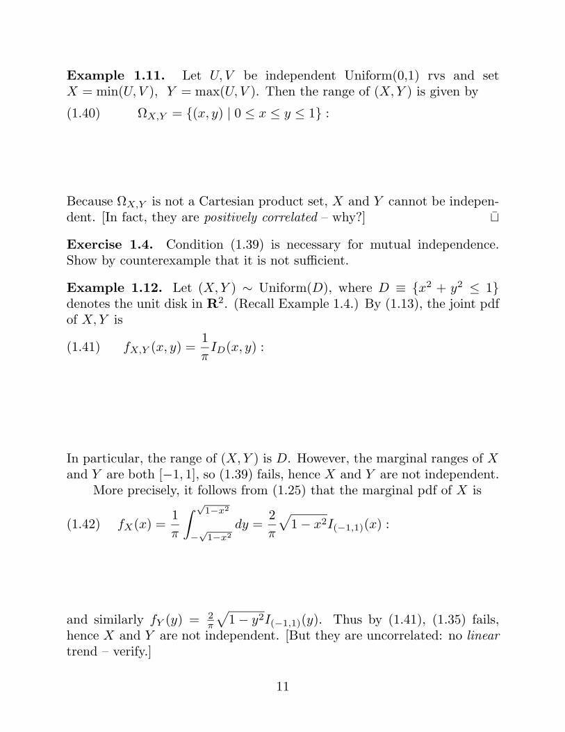
Example 1.11. Let U, V be independent Uniform(0,1) rvs and setX = min(U, V ), Y = max(U, V ). Then the range of (X, Y ) is given by
(1.40) ΩX,Y = (x, y) | 0 ≤ x ≤ y ≤ 1 :
Because ΩX,Y is not a Cartesian product set, X and Y cannot be indepen-dent. [In fact, they are positively correlated – why?]
Exercise 1.4. Condition (1.39) is necessary for mutual independence.Show by counterexample that it is not sufficient.
Example 1.12. Let (X, Y ) ∼ Uniform(D), where D ≡ x2 + y2 ≤ 1denotes the unit disk in R2. (Recall Example 1.4.) By (1.13), the joint pdfof X, Y is
(1.41) fX,Y (x, y) =1π
ID(x, y) :
In particular, the range of (X, Y ) is D. However, the marginal ranges of Xand Y are both [−1, 1], so (1.39) fails, hence X and Y are not independent.
More precisely, it follows from (1.25) that the marginal pdf of X is
(1.42) fX(x) =1π
∫ √1−x2
−√
1−x2dy =
2π
√1 − x2I(−1,1)(x) :
and similarly fY (y) = 2π
√1 − y2I(−1,1)(y). Thus by (1.41), (1.35) fails,
hence X and Y are not independent. [But they are uncorrelated: no lineartrend – verify.]
11
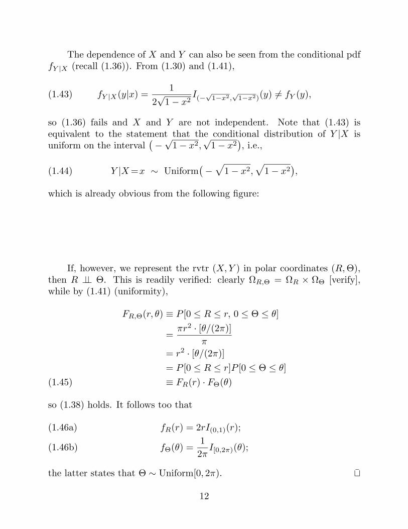
The dependence of X and Y can also be seen from the conditional pdffY |X (recall (1.36)). From (1.30) and (1.41),
(1.43) fY |X(y|x) =1
2√
1 − x2I(−
√1−x2,
√1−x2)(y) = fY (y),
so (1.36) fails and X and Y are not independent. Note that (1.43) isequivalent to the statement that the conditional distribution of Y |X isuniform on the interval
(−
√1 − x2,
√1 − x2
), i.e.,
(1.44) Y |X =x ∼ Uniform(−
√1 − x2,
√1 − x2
),
which is already obvious from the following figure:
If, however, we represent the rvtr (X, Y ) in polar coordinates (R, Θ),then R ⊥⊥ Θ. This is readily verified: clearly ΩR,Θ = ΩR × ΩΘ [verify],while by (1.41) (uniformity),
FR,Θ(r, θ) ≡ P [0 ≤ R ≤ r, 0 ≤ Θ ≤ θ]
=πr2 · [θ/(2π)]
π
= r2 · [θ/(2π)]= P [0 ≤ R ≤ r]P [0 ≤ Θ ≤ θ]≡ FR(r) · FΘ(θ)(1.45)
so (1.38) holds. It follows too that
fR(r) = 2rI(0,1)(r);(1.46a)
fΘ(θ) =12π
I[0,2π)(θ);(1.46b)
the latter states that Θ ∼ Uniform[0, 2π).
12

Mutual independence. Events A1, . . . , An (n ≥ 3) are mutually independentiff
(1.47) P (Aε11 ∩ · · · ∩ Aεn
n ) = P (Aε11 ) · · ·P (Aεn
n ) ∀(ε1, . . . , εn) ∈ 0, 1n,
where A1 := A and A0 := Ac. A finite family2 of rvs X1, . . . , Xn aremutually independent iff X1 ∈ B1, . . . , Xn ∈ Bn are mutually indepen-dent for every choice of measurable events B1, . . . , Bn. An infinite familyX1, X2, . . . of rvs are mutually independent iff every finite subfamily is mu-tually independent. Intuitively, mutual independence of rvs means thatinformation about the values of some of the rvs does not change the (joint)probability distribution of the other rvs.
Exercise 1.5. (i) For n ≥ 3 events A1, . . . , An, show that mutual inde-pendence implies pairwise independence. (ii) Show by counterexample thatpairwise independence does not imply mutual independence. (iii) Show that
(1.48) P (A ∩ B ∩ C) = P (A)P (B)P (C)
is not by itself sufficient for mutual independence of A, B, C.
Example 1.13. In Example 1.1, suppose that the n trials are mutuallyindependent and that p : P (H) and q ≡ (1 − p) ≡ P (T ) do not vary fromtrial to trial. Let X denote the total number of Heads in the n trials. Thenby independence, X ∼ Binomial(n, p), i.e., the pmf pX of X is given by(1.2). [Verify!].
Example 1.14. In Example 1.2, suppose that the entire infinite sequenceof trials are mutually independent and that p := P (H) does not vary fromtrial to trial. Let X denote the number of trials needed to obtain the firstHead. Then by independence, X ∼ Geometric(p), i.e., the pmf pX is givenby (1.3). [Verify!]
Mutual independence of rvs X1, . . . , Xn can be expressed in terms oftheir joint pmf (discrete case), joint pdf (continuous case), or joint cdf (both
2 More precisely, (X1, . . . , Xn) must be a rvtr, i.e., X1, . . . , Xn arise from the
same random experiment.
13
cases): X1, . . . , Xn are mutually independent iff either
fX1,...,Xn(x1, . . . , xn) = fX1(x1) · · · fXn(xn);(1.49)FX1,...,Xn(x1, . . . , xn) = FX1(x1) · · ·FXn(xn).(1.50)
Again, these conditions implicity require that the joint range of X1, . . . , Xn
is the Cartesian product of the marginal ranges:
(1.51) ΩX1,...,Xn = ΩX1 × · · · × ΩXn .
Example 1.15. Continuing Example 1.13, let X1, . . . , Xn be indicatorvariables (≡ Bernoulli variables) that denote the outcomes of trials 1, . . . , n:Xi = 1 or 0 according to whether Heads or Tails occurs on the ith trial. HereX1, . . . , Xn are mutually independent and identically distributed (i.i.d.) rvs,and X can be represented as their sum: X = X1 + · + Xn. Therefore weexpect that X and X1 are not independent. In fact, the joint range
ΩX,X1 = (x, x1) | x = 0, 1, . . . , n, x1 = 0, 1, x ≥ x1.
The final inequality implies that this is not a Cartesian product of an x-setand an x1-set [verify], hence by (1.39), X and X1 cannot be independent.
1.6. Composite events and total probability.
Equation (1.27) can be rewritten in the following useful form(s):
(1.52) P (A ∩ B) = P [A | B]P (B)(
= P [B | A]P (A)).
By (1.28) and (1.30), similar formulas hold for joint pmfs and pdfs:
(1.53) f(x, y) = f(x|y)f(y)(
= f(y|x)f(x)).
Now suppose that the sample space Ω is partitioned into a finite or countableset of disjoint events: Ω = ∪∞
i=1Bi. Then by the countable additivity of Pand (1.52), we have the law of total probability:
P (A) = P[A ∩
(∪∞
i=1 Bi
)]= P
[∪∞
i=1
(A ∩ Bi
)]=
∞∑i=1
P [A ∩ Bi] =∞∑
i=1
P [A | Bi]P (Bi).(1.54)
14
Example 1.16. Let X ∼ Poisson(λ), where λ > 0 is unknown and is to beestimated. (For example, λ might be the decay rate of a radioactive processand X the number of emitted particles recorded during a unit time interval.)We shall later see that the expected value of X is given by E(X) = λ, so ifX were observed then we would estimate λ by λ ≡ X.
Suppose, however, that we do not observe X but instead only observethe value of Y , where
(1.55) Y |X =x ∼ Binomial(n = x, p).
(This would occur if each particle emitted has probability p of being ob-served, independently of the other emitted particles.) If p is known then wemay still obtain a reasonable estimate of λ based on Y , namely λ = 1
pY .To obtain the distribution of Y , apply (1.54) as follows (set q = (1−p)):
P [Y = y] = P [Y = y, X = y, y + 1, . . .] [since X ≥ Y ]
=∞∑
x=y
P [Y = y | X = x] · P [X = x] [by (1.54)]
=∞∑
x=y
(x
y
)pyqx−y · e−λ λx
x![by (1.2), (1.4)]
=e−λ(pλ)y
y!
∞∑k=0
(qλ)k
k![let k = x − y]
=e−pλ(pλ)y
y!.(1.56)
This implies that Y ∼ Poisson(pλ), so
E(λ) ≡ E(1pY ) =
1pE(Y ) =
1p(pλ) = λ,
which justifies λ as an estimate of λ based on Y .
15
1.7. Bayes formula.
If P (A) > 0 and P (B) > 0, then (1.27) yields Bayes formula for events:
(1.57) P [A | B] =P [A ∩ B]
P (B)=
P [B | A]P (A)P (B)
.
Similarly, (1.28) and (1.30) yield Bayes formula for joint pmfs and pdfs:
(1.58) f(x|y) =f(y|x)f(x)
f(y)if f(x), f(y) > 0.
[See §4 for extensions to the mixed cases where X is discrete and Y iscontinuous, or vice versa.]
Example 1.17. In Example 1.16, what is the conditional distribution ofX given that Y = y? By (1.58), the conditional pmf of X | Y = y is
f(x|y) =
(xy
)pyqx−y · e−λλx/x!
e−pλ(pλ)y/y!
=e−qλ(qλ)x−y
(x − y)!, x = y, y + 1, . . . .
Thus, if we set Z = X − Y , then
(1.59) P [Z = z | Y = y] =e−qλ(qλ)z
z!, z = 0, 1, . . . ,
so Z | Y =y ∼ Poisson(qλ). Because this conditional distribution does notdepend on y, it follows from (1.36) that X − Y ⊥⊥ Y . (In the radioactivityscenario, this states that the number of uncounted particles is independentof the number of counted particles.)Note: this also shows that if U ∼ Poisson(µ) and V ∼ Poisson(ν) with Uand V independent, then U + V ∼ Poisson(µ + ν). [Why?]
16
Exercise 1.6. (i) Let X and Y be independent Bernoulli rvs with
P [X = 1] = p, P [X = 0] = 1 − p;P [Y = 1] = r, P [Y = 0] = 1 − r.
Let Z = X + Y , a discrete rv with range 0, 1, 2. Do there exist p, r suchthat Z is uniformly distributed on its range, i.e., such that P [Z = k] = 1
3for k = 0, 1, 2? (Prove or disprove.)
(ii)* (unfair dice.) Let X and Y be independent discrete rvs, each havingrange 1, 2, 3, 4, 5, 6, with pmfs
pX(k) = pk, pY (k) = rk, k = 1, . . . , 6.
Let Z = X + Y , a discrete rv with range 2, 3, 4, 5, 6, 7, 8, 9, 10, 11, 12.First note that if X and Y are the outcomes of tossing two fair dice, i.e.pX(k) = pY (k) = 1
6 for k = 1, . . . , 6, then the pmf of Z is given by
136
,236
,336
,436
,536
,636
,536
,436
,336
,236
,136
,
which is not uniform over its range. Do there exist unfair dice such thatZ is uniformly distributed over its range, i.e., such that P [Z = k] = 1
11 fork = 2, 3, . . . , 12? (Prove or disprove.)
1.8. Conditional independence.
Consider three events A, B, C with P (C) > 0. We say that A and Bare conditionally independent given C, written A ⊥⊥ B | C, if any of thefollowing three equivalent conditions hold (recall (1.32) - (1.34)):
P [A ∩ B | C] = P [A | C]P [B | C];(1.60)P [A | B, C] = P [A | C];(1.61)P [B | A, C] = P [B | C].(1.62)
As with ordinary independence, A ⊥⊥ B | C ⇔ A ⊥⊥ Bc | C ⇔ Ac ⊥⊥ B | C⇔ Ac ⊥⊥ Bc | C (see Exercise 1.3). However, A ⊥⊥ B | C ⇔ A ⊥⊥ B | Cc
[Examples are easy – verify].
17
The rvs X and Y are conditionally independent given Z, denoted asX ⊥⊥ Y | Z, if
(1.63) X ∈ A ⊥⊥ Y ∈ B | Z ∈ C
for each triple of (measurable) events A, B, C. It is straightforward to showthat for a jointly discrete or jointly continuous trivariate rvtr (X, Y, Z),X ⊥⊥ Y | Z iff any of the following three equivalent conditions hold [verify]:
f(x, y | z) = f(x | z)f(y | z);(1.64)f(y | x, z) = f(y | z);(1.65)f(x | y, z) = f(x | z);(1.66)
f(x, y, z)f(z) = f(x, z)f(y, z);(1.67)
Exercise 1.7. Conditional independence ⇔ independence.
(i) Construct (X, Y, Z) such that X ⊥⊥ Y | Z but X ⊥⊥ Y .
(ii) Construct (X, Y, Z) such that X ⊥⊥ Y but X ⊥⊥ Y | Z.
Graphical Markov model representation of X ⊥⊥ Y | Z:
(1.68) X < −−−Z −−− > Y.
18
2. Transforming Continuous Distributions.
2.1. One function of one random variable.
Let X be a continuous rv with pdf fX on the range ΩX = (a, b)(−∞ ≤ a < b ≤ ∞). Define the new rv Y = g(X), where g is a strictlyincreasing and continuous function on (a, b). Then the pdf fY is determinedas follows:
Theorem 2.1.
(2.1) fY (y) =
fX(g−1(y))g′(g−1(y)) , g(a) < y < g(b);0, otherwise.
Proof.
fY (y) =d
dyFY (y)
=d
dyP [Y ≤ y]
=d
dyP [g(X) ≤ y](2.2)
=d
dyP [X ≤ g−1(y)]
=d
dyFX(g−1(y))
= fX(g−1(y))d
dyg−1(y)
= fX(g−1(y))1
g′(g−1(y)). [why?]
Example 2.1. Consider g(x) = x2. In order that this g be strictly increas-ing we must have 0 ≤ a. Then g′(x) = 2x and g−1(y) =
√y, so from (2.1)
with Y = X2,
(2.3) fY (y) =1
2√
yfX(
√y), a2 < y < b2.
19
In particular, if X ∼ Uniform(0, 1) then Y ≡ X2 has pdf
(2.4) fY (y) =1
2√
y, 0 < y < 1. [decreasing]
Example 2.2a. If X has cdf F then Y ≡ F (X) ∼ Uniform(0, 1). [Verify]
Example 2.2b. How to generate a rv Y with a pre-specified pdf f :
Solution: Let F be the cdf corresponding to f . Use a computer to generateX ∼ Uniform(0, 1) and set Y = F−1(X). Then Y has cdf F . [Verify]
Note: If g is strictly decreasing then (2.1) remains true with g′(g−1(y))replaced by |g′(g−1(y))| [Verify].
Now suppose that g is not monotone. Then (2.2) remains valid, butthe region g(X) ≤ y must be specifically determined before proceeding.
Example 2.3. Again let Y = X2, but now suppose that the range of X is(−∞,∞). Then for y > 0,
fY (y) =d
dyP [Y ≤ y]
=d
dyP [X2 ≤ y]
=d
dyP [−√
y ≤ X ≤ √y]
=d
dy
[FX(
√y) − FX(−√
y)]
=1
2√
y
[fX(
√y) + fX(−√
y)].(2.5)
If in addition the distribution of X is symmetric about 0, i.e., fX(x) =fX(−x), then (2.5) reduces to
(2.6) fY (y) =1√yfX(
√y).
20
Note that this is similar to (2.3) (where the range of X was restricted to(0,∞)) but without the factor 1
2 . To understand this, consider
X1 ∼ Uniform(0, 1), X2 ∼ Uniform(−1, 1).
ThenfX1(x) = I(0,1)(x), fX2(x) = 1
2I(−1,1)(x),
but Yi = X2i has pdf 1
2√
y I(0,1) for i = 1, 2. [Verify – recall (2.4)].
Example 2.4. Let X ∼ N(0, 1), i.e., fX(x) = 1√2π
e−x2/2I(−∞,∞)(x) andY = X2. Then by (2.6),
(2.7) fY (y) =1√2π
y−1/2e−y/2I(0,∞)(y),
the Gamma( 12 , 1
2 ) pdf, which is also called the chi-square pdf with one degreeof freedom, denoted as χ2
1 (see Remark 6.3). Note that (2.7) shows that[verify!]
(2.8) Γ(
12
)=
√π.
Exercise 2.1. Let Θ ∼ Uniform(0, 2π), so we may think of Θ as a randomangle. Define X = cos Θ. Find the pdf fX .
Hint: Always begin by specifying the range of X, which is [−1, 1] here. Onthis range, what shape do you expect fX to have, among the following threepossibilities? (Compare this fX to that in Example 1.12, p. 11.)
21
Exercise 2.1 suggests the following problem. A bivariate pdf fX,Y onR2 is called radial if it has the form
(2.9) fX,Y (x, y) = g(x2 + y2)
for some (non-negative) function g on (0,∞). Note that the condition∫∫R2
f(x, y)dxdy = 1
requires that
(2.10)∫ ∞
0
rg(r2)dr =12π
[why?]
Exercise 2.2*. Does there exist a radial pdf fX,Y on the unit disk in R2
such that the marginal distribution of X is Uniform(−1, 1)? More precisely,does there exist g on (0, 1) that satisfies (2.10) and
(2.11) fX(x) ≡∫ √
1−x2
−√
1−x2g(x2 + y2)dy = 1
2I(−1,1)(x)?
Note: if such a radial pdf fX,Y on the unit disk exists, it could be called abivariate uniform distribution, since both X and Y (by symmetry) have theUniform(−1, 1) distribution. Of course, there are simpler bivariate distri-butions with these uniform marginal distributions but which are not radialon the unit disk. [Can you think of two?]
22
2.2. One function of two or more random variables.
Let (X, Y ) be a continuous bivariate rvtr with pdf fX,Y on a subset of R2.Define a new rv
U = g(X, Y ), e.g., U = X + Y, X − Y,X
Y,
1 + exp (X + Y )1 + exp (X − Y )
.
Then the pdf fU can be determined via two methods:
Method One: Apply
(2.12) fU (u) =d
duFU (u) =
d
duP [U ≤ u] =
d
duP [g(X, Y ) ≤ u],
then determine the region (X, Y ) | g(X, Y ) ≤ u.
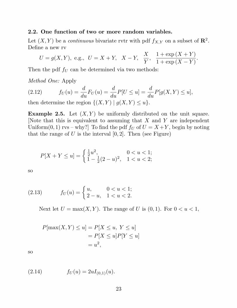
Example 2.5. Let (X, Y ) be uniformly distributed on the unit square.[Note that this is equivalent to assuming that X and Y are independentUniform(0, 1) rvs – why?] To find the pdf fU of U = X+Y , begin by notingthat the range of U is the interval [0, 2]. Then (see Figure)
P [X + Y ≤ u] =
12u2, 0 < u < 1;1 − 1
2 (2 − u)2, 1 < u < 2;
so
(2.13) fU (u) =
u, 0 < u < 1;2 − u, 1 < u < 2.
Next let U = max(X, Y ). The range of U is (0, 1). For 0 < u < 1,
P [max(X, Y ) ≤ u] = P [X ≤ u, Y ≤ u]= P [X ≤ u]P [Y ≤ u]
= u2,so
(2.14) fU (u) = 2uI(0,1)(u).
23
Finally, let V = min(X, Y ). Again the range of V is [0, 1], and for0 < v < 1,
P [min(X, Y ) ≤ v] = 1 − P [min(X, Y ) > v]= 1 − P [X > v, Y > v]= 1 − P [X > v]P [Y > v]
= 1 − (1 − v)2,so
(2.15) fV (v) = 2(1 − v)I(0,1)(v).
Exercise 2.3*. Let X, Y, Z be independent, identically distributed (i.i.d.)Uniform(0, 1) rvs. Find the pdf of U ≡ X + Y + Z. [What is range(U)?]
Example 2.6. Let X, Y be i.i.d. Exponential(1) rvs and set U = X + Y .Then for 0 < u < ∞,
P [X + Y ≤ u] =∫∫
x+y≤u
e−x−ydxdy
=∫ u
0
e−x[ ∫ u−x
0
e−ydy]dx
=∫ u
0
e−x[1 − e−(u−x)
]dx
=∫ u
0
e−xdx − e−u
∫ u
0
dx
= 1 − e−u − ue−u,
so by (2.12),
(2.16) fU (u) =d
du[1 − e−u − ue−u] = ue−u.
Next let V = min(X, Y ). Then for 0 < v < ∞,
P [min(X, Y ) ≤ v] = 1 − P [min(X, Y ) > v]= 1 − P [X > v, Y > v]
= 1 −[ ∫ ∞
v
e−xdx][ ∫ ∞
v
e−ydy]
= 1 − e−2v,
24
so
(2.17) fV (v) = 2e−2v,
that is, V ≡ min(X, Y ) ∼ Exponential(2).
More generally: If X1, . . . , Xn are i.i.d. Exponential(λ) rvs, then [verify!]
(2.18) min(X1, . . . , Xn) ∼ Exponential(nλ).
However: if T = max(X, Y ), then T is not an exponential rv [verify!]:
(2.19) fT (t) = 2(e−t − e−2t
).
Now let Z = |X − Y | ≡ max(X, Y ) − min(X, Y ). The range of Z is(0,∞). For 0 < z < ∞,
P [|X − Y | ≤ z]=1 − P [Y ≥ X + z] − P [Y ≤ X − z]=1 − 2P [Y ≥ X + z] [by symmetry]
=1 − 2∫ ∞
0
e−x[ ∫ ∞
x+z
e−ydy]dx
=1 − 2∫ ∞
0
e−xe−(x+z)dx
=1 − 2e−z
∫ ∞
0
e−2xdx
=1 − e−z,
so
(2.20) fZ(z) = e−z.
That is, Z ≡ max(X, Y )−min(X, Y ) ∼ Exponential(1), the same as X andY themselves.
Note: This is another “memory-free” property of the exponential distri-bution. It is stronger in that it involves a random starting time, namelymin(X, Y ).
25
Finally, let W = XX+Y . The range of W is (0, 1). For 0 < w < 1,
P[ X
X + Y≤ w
]=P [X ≤ w(X + Y )]
=P[Y ≥
(1 − w
w
)X
]=
∫ ∞
0
[ ∫ ∞(1−w
w
)x
e−y]e−xdx
=∫ ∞
0
[e−
(1−w
w
)xe−xdx
]=
∫ ∞
0
e−xw dx
= w,
so
(2.21) fW (w) = I(0,1)(w),
that is, W ≡ XX+Y ∼ Uniform(0, 1).
Note: In Example 6.3 we shall show that XX+Y ⊥⊥ (X + Y ). Then (2.21)
can be viewed as a “backward” memory-free property of the exponentialdistribution: given X + Y , the location of X is uniformly distributed overthe interval (0, X + Y ).
Method Two: Introduce a second rv V = h(X, Y ), where h is chosen cleverlyso that it is relatively easy to find the joint pdf fU,V via the “Jacobianmethod”, then marginalize to find fU . (This method appears in §6.2.)
26
3. Expected Value of a RV: Mean, Variance, Covariance; MomentGenerating Function; Normal & Poisson Approximations.
The expected value (expectation, mean) of a rv X is defined by
EX =∑
x
xfX(x), [discrete case](3.1)
EX =∫
xfX(x) dx, [continuous case](3.2)
provided that the sum or integral is absolutely convergent. If not convergent,then the expectation does not exist.
The Law of Large Numbers states that if EX exists, then for i.i.d.copies X1, X2, . . . , of X the sample averages Xn ≡ 1
n
∑ni=1 Xi converge to
EX as n → ∞. If the sum in (3.1) or integral in (3.2) equals +∞ (−∞),then Xn → +∞ (−∞). If the sum or integral has no value (i.e. has theform ∞−∞), then Xn will oscillate indefinitely.
If the probability distribution of X is thought of as a (discrete or con-tinuous) mass distribution on R1, then EX is just the center of gravity ofthe mass. With this interpretation, we can often use symmetry to find theexpected value without actually calculating the sum or integral; however,absolute convergence still must be verified! [Eg. Cauchy distribution]
Example 3.1: [verify, including convergence; for Var see (3.9) and (3.10)]
X ∼ Binomial(n, p) ⇒ EX = np, VarX = np(1 − p); [sum]
X ∼ Geometric(p) ⇒ EX = 1/p, VarX = (1 − p)2/p; [sum]X ∼ Poisson(λ) ⇒ EX = λ, VarX = λ; [sum]
X ∼ Exponential(λ) ⇒ EX = 1/λ, VarX = 1/λ2; [integrate]X ∼ Normal N(0, 1) ⇒ EX = 0, VarX = 1; [symmetry, integrate]X ∼ Cauchy C(0, 1) ⇒ EX and VarX do not exist;
X ∼ Gamma(α, λ) ⇒ EX = α/λ, VarX = α/λ2; [integrate]X ∼ Beta(α, β) ⇒ EX = α/(α + β); [integrate]
X ∼ std. Logistic ⇒ EX = 0 [symmetry]
X ∼ Uniform(a, b) ⇒ EX =a + b
2,VarX =
(b − a)2
12; [symm., integ.]
27
The expected value E[g(X)] of a function of a rv X is defined similarly:
E[g(X)] =∑
x
g(x)fX(x), [discrete case](3.3)
E[g(X)] =∫
g(x)fX(x) dx, [continuous case](3.4)
In particular, the rth moment of X (if it exists) is defined as E(Xr), r ∈ R1.
Expectations of functions of random vectors are defined similarly. Forexample in the bivariate case,
E[g(X, Y )] =∑
x
∑y
g(x, y)fX,Y (x, y), [discrete case](3.5)
E[g(X, Y )] =∫ ∫
g(x, y)fX,Y (x, y) dxdy, [continuous case](3.6)
Linearity: It follows from (3.5) and (3.6) that expectation is linear:
(3.7) E[ag(X, Y ) + bh(X, Y )] = aE[g(X, Y )] + bE[h(X, Y )]. [verify]
Order-preserving: X ≥ 0 ⇒ EX ≥ 0 (and EX = 0 iff X ≡ 0).
X ≥ Y ⇒ EX ≥ EY (and EX = EY iff X ≡ Y ). [Pf: EX−EY = E(X−Y )]
Linearity (≡ additivity) simplifies many calculations:
Binomial mean: We can find the expected value of X ∼ Binomial(n, p) eas-ily as follows: Because X is the total number of successes in n independentBernoulli trials, i.e., trials with exactly two outcomes (H,T, or S,F, etc.),we can represent X as
(3.8) X = X1 + · · · + Xn,
where Xi = 1 (or 0) if S (or F) occurs on the ith trial. (Recall Example1.15.) Thus by linearity,
EX = E(X1 + · · · + Xn) = EX1 + · · · + EXn = p + · · · + p = np.
28
Variance. The variance of X is defined to be
(3.9) VarX = E[(X − EX)2],
the average of the square of the deviation of X about its mean. The standarddeviation of X is
sd (X) =√
VarX.
Properties.(a) VarX ≥ 0; equality holds iff X is degenerate (constant).
Var(aX + b) = a2 VarX;(b) location − scale :sd (aX + b) = |a| · sd (X).
VarX ≡ E[(X − EX)2] = E[X2 − 2XEX + (EX)2](c)= E(X2) − 2(EX)(EX) + (EX)2
= E(X2) − (EX)2.(3.10)
The standard deviation is a measure of the spread ≡ dispersion of thedistribution of X about its mean value. An alternative measure of spreadis E[|X − EX|]. Another measure of spread is the difference between the75th and 25th percentiles of the distribution of X.
Covariance: The covariance between X and Y indicates the nature of thelinear dependence (if any) between X and Y :
(3.11) Cov(X, Y ) = E[(X − EX)(Y − EY )]. [interpret; also see §4]
29
Properties of covariance:
(a) Cov(X, Y ) = Cov(Y, X).
Cov(X, Y ) = E[XY − XEY − Y EX + (EX)(EY )](b)= E(XY ) − 2(EX)(EY ) + (EX)(EY )= E(XY ) − (EX)(EY ).(3.12)
(c) Cov(X, X) = VarX.
(d) If X or Y is a degenerate rv (a constant), then Cov(X, Y ) = 0.
(e) Bilinearity: Cov(aX, bY + cZ) = ab Cov(X, Y ) + ac Cov(X, Z).
Cov(aX + bY, cZ) = ac Cov(X, Z) + bc Cov(Y, Z).
(f) Variance of a sum or difference:
(3.13) Var(X ± Y ) = VarX + VarY ± 2 Cov(X, Y ). [verify]
(g) Product rule. If X and Y are independent it follows from (1.35), (3.5)and (3.6) that
(3.14) E[g(X)h(Y )] = E[g(X)] · E[h(Y )]. [verify]
Thus, by (3.12) and (3.13),
X ⊥⊥ Y ⇒ Cov(X, Y ) = 0,(3.15)X ⊥⊥ Y ⇒ Var(X ± Y ) = VarX + VarY.(3.16)
Exercise 3.1. Show by counterexample that the converse of (3.15) is nottrue. [Example 1.12 provides one counterexample: Suppose that (X, Y )is uniformly distributed over the unit disk D. Then by the symmetry ofD, (X, Y ) ∼ (X,−Y ). Thus Cov(X, Y ) = Cov(X,−Y ) = −Cov(X, Y ), soCov(X, Y ) = 0. But we have already seen that X/⊥⊥Y .]
Binomial variance: We can find the variance of X ∼ Binomial(n, p) easilyas follows (recall Example 1.12):
VarX = Var(X1 + · · · + Xn) [by (3.8)]= VarX1 + · · · + VarXn [by (3.16)]= p(1 − p) + · · · + p(1 − p) [by (3.10)]= np(1 − p).(3.17)
30
Variance of a sample average ≡ sample mean: Let X1, . . . , Xn be i.i.d. rvs,each with mean µ and variance σ2 < ∞ and set Xn = 1
n (X1 + · · · + Xn).Then by (3.16),
(3.18) E(Xn) = µ, Var(Xn) =Var(X1 + · · · + Xn)
n2=
nσ2
n2=
σ2
n.
3.1. The Weak Law of Large Numbers (WLLN).
Let X1, . . . , Xn be i.i.d. rvs, each with mean µ and variance σ2 < ∞. ThenXn converges to µ in probability (Xn
p→ µ), that is, for each ε > 0,
P [|Xn − µ| ≤ ε] → 1 as n → ∞.
Proof. By Chebyshev’s Inequality (below) and (3.18),
P [|Xn − µ| ≥ ε] ≤ Var(Xn)ε2
=σ2
nε2→ 0 as n → ∞.
Lemma 3.1. Chebyshev’s Inequality. Let EY = ν, VarY = τ2. Then
(3.19) P [|Y − ν| ≥ ε] ≤ τ2
ε2.
Proof. Let X = Y − ν, so E(X) = 0. Assume that X is continuous withpdf f . (The discrete case is similar, with sums replacing integrals.) Then
τ2 ≡ E(X2) =∫|x|≥ε
x2f(x)dx +∫|x|<ε
x2f(x)dxy
≥∫|x|≥ε
ε2f(x)dx = ε2P [|X| ≥ ε].
Example 3.2. Sampling without replacement - the hypergeometricdistribution.
Suppose an urn contains r red balls and w white balls. Draw n balls atrandom from the urn and let X denote the number of red balls obtained.If the balls are sampled with replacement, then clearly X ∼ Binomial(n, p),where p = r/(r + w), so EX = np, VarX = np(1 − p).
31
Suppose, however, that the balls are sampled without replacement.Note that we now require that n ≤ r + w. The probability distributionof X is described as follows: its range is max(0, n − w) ≤ x ≤ min(r, n)[why?], and its pmf is given by
(3.20) P [X = x] =
(rx
)(w
n−x
)(r+w
n
) , max(0, n − w) ≤ x ≤ min(r, n).
[Verify the range and verify the pmf. This probability distribution is calledhypergeometric because these ratios of binomial coefficients occurs as thecoefficients in the expansion of hypergeometric functions such as Besselfunctions. The name is unfortunate because it has no relationship to theprobability model that gives rise to (3.20).]
To determine EX and VarX, rather than combining (3.1) and (3.20),it is easier again to use the representation
X = X1 + · · · + Xn,
where, as in (3.8), Xi = 1 (or 0) if a red (or white) ball is obtained onthe ith trial. Unlike (3.13), however, clearly X1, . . . , Xn are not mutuallyindependent. [Why?] Nonetheless, the joint distribution of (X1, . . . , Xn) isexchangeable ≡ symmetric ≡ permutation-invariant, that is
(X1, . . . , Xn) ∼ (Xi1 , . . . , Xin)
for every permutation (i1, . . . , in) of (1, . . . , n). This is intuitively evidentbut we will not prove it. As supporting evidence, however, note that
P [X2 = 1] = P [X2 = 1|X1 = 1]P [X1 = 1] + P [X2 = 1|X1 = 0]P [X1 = 0]
=r − 1
r + w − 1· r
r + w+
r
r + w − 1· w
r + w
=r
r + w≡ P [X1 = 1],(3.21)
so X1 ∼ X2. Note too that since X1X2 has range 0, 1,E(X1X2) = P [X1X2 = 1]
= P [X1 = 1, X2 = 1]= P [X2 = 1|X1 = 1]P [X1 = 1]
=r − 1
r + w − 1r
r + w,
32
Cov(X1, X2) = E(X1X2) − (EX1)(EX2)
=r − 1
r + w − 1r
r + w−
[ r
r + w
]2
=r
r + w
[ r − 1r + w − 1
− r
r + w
]=
−rw
(r + w)2(r + w − 1).(3.22)
[Thus X1 and X2 are negatively correlated, which is intuitively clear. [Why?]
By (3.21) and exchangeability, EXi = rr+w ≡ p for i = 1, . . . , n, so
(3.23) EX = EX1 + · · ·EXn = n( r
r + w
)≡ np,
the same as for sampling with replacement.
Key question: do we expect VarX also to be the same as for sampling withreplacement, namely, np(1 − p)? Larger? Smaller?
Answer: By (3.22) and exchangeability,
VarX =n∑
i=1
VarXi + 2∑
1≤i<j≤n
Cov(Xi, Xj)
= np(1 − p) + n(n − 1)Cov(X1, X2)
= nr
r + w
w
r + w+ n(n − 1)
[ −rw
(r + w)2(r + w − 1)
]=
nrw
(r + w)2[1 − n − 1
r + w − 1
]= np(1 − p)
[1 − n − 1
N − 1
],(3.24)
where N ≡ r + w is the total number of balls in the urn. [Discuss n−1N−1 .]
By comparing (3.24) to (3.17), we see that sampling without replace-ment from a finite population reduces the variability of the outcome. This isto be expected from the representation X = X1 + · · ·+Xn and the fact thateach pair (Xi, Xj) is negatively correlated (by (3.22) and exchangeability).
33
3.2. Correlated and conditionally correlated events.
The events A and B are positively correlated if any of the following threeequivalent conditions hold:
P [A ∩ B] > P [A]P [B];(3.25)P [A | B] > P [A];(3.26)P [B | A] > P [B].(3.27)
Note that (3.25) is equivalent to Cov(IA, IB) > 0. Negative correlation isdefinined similarly with > replaced by <.
It is easy to see that A and B are positively correlated iff [verify:]
either P [A | B] > P [A | Bc](3.28)or P [B | A] > P [B | Ac].(3.29)
The events A and B are conditionally positively correlated given C ifany of the following three equivalent conditions hold:
P [A ∩ B | C] > P [A | C]P [B | C];(3.30)P [A | B, C] > P [A | C];(3.31)P [B | A, C] > P [B | C].(3.32)
Then A and B are positively correlated given C iff [verify:]
either P [A | B, C] > P [A | Bc, C](3.33)or P [B | A, C] > P [B | Ac, C].(3.34)
Example 3.3: Simpson’s paradox.
(3.35)
P [A | B, C] > P [A | Bc, C]
P [A | B, Cc] > P [A | Bc, Cc]
⇒ P [A | B] > P [A | Bc] !
To see this, consider the famous Berkeley Graduate School Admissions data.To simplify, assume there are only two graduate depts, Physics and English.
34
LetA = Applicant is Accepted to Berkeley Grad SchoolB = Applicant is Female ≡ F
Bc = Applicant is Male ≡ M
C = Applied to Physics Department ≡ Ph
Cc = Applied to English Department ≡ En.
Physics: 100 F Applicants, 60 Accepted: P [A | F, Ph] = 0.6.
Physics: 100 M Applicants, 50 Accepted: P [A | M, Ph] = 0.5.
English: 1000 F Applicants, 250 Accepted: P [A | F, En] = 0.25.
English: 100 M Applicants, 20 Accepted: P [A | M, En] = 0.2.
Total: 1100 F Applicants, 310 Accepted: P [A | F ] = 0.28.
Total: 200 M Applicants, 70 Accepted: P [A | M ] = 0.35.
Therefore: P [A | F ] < P [A | M ]. Is this evidence of discrimination?
No :P [A | F, Ph] > P [A | M, Ph],P [A | F, En] > PA | M, En],
so F’s are more likely to be accepted into each dept Ph and En separately!
Explanation: Most F’s applied to English, where the overall acceptance rateis low:
P [A | F ] = P [A | F, Ph]P [Ph | F ] + P [A | F, En]P [En | F ],
P [A | M ] = P [A | M, Ph]P [Ph | M ] + P [A | M, En]P [En | M ].
Exercise 3.2. Show that the implication (3.35) does hold if B ⊥⊥ C.
35
3.3. Moment generating functions: they uniquely determine mo-ments, distributions, and convergence of distributions.
The moment generating function (mgf) of (the distribution of) the rv X is:
(3.36) mX(t) = E(etX
), −∞ < t < ∞.
Clearly mX(0) = 1 and 0 < mX(t) ≤ ∞, with ∞ possible. If mX(t) < ∞for |t| < δ then the Taylor series expansion of etX yields
(3.37) mX(t) = E[ ∞∑
k=0
(tX)k
k!
]=
∞∑k=0
tk
k!E(Xk), |t| < δ,
a power series whose coefficients are the kth moments of X. In this case themoments of X are recovered from the mgf mX by differentiation at t = 0:
(3.38) E(Xk) = m(k)X (0), k = 1, 2, .... [verify]
Location-scale:
(3.39) maX+b(t) = E(et(aX+b)
)= ebtE
(eatX
)= ebtmX(at).
Multiplicativity: X, Y independent ⇒
(3.40) mX+Y (t) = E(et(X+Y )
)= E
(etX
)E
(etY
)= mX(t)mY (t).
In particular, if X1, . . . , Xn are i.i.d. then
(3.41) mX1+···+Xn(t) = [mX1(t)]
n.
Example 3.4.
Bernoulli (p): Let X =
1, with probability p;0, with probability 1-p. Then
(3.42) mX(t) = pet + (1 − p).
Binomial (n, p): We can represent X = X1 + · · · + Xn, where X1, . . . , Xn
are i.i.d. Bernoulli(p) 0-1 rvs. Then by (3.41) and (3.42),
(3.43) mX(t) =[pet + (1 − p)
]n.
36
Poisson (λ):
(3.44) mX(t) = e−λ∞∑
k=0
λk
k!etk = e−λeλet
= eλ(et−1).
Standard univariate normal N(0, 1):
mX(t) =1√2π
∫ ∞
−∞etxe−
x22 dx
= et2/2 1√2π
∫ ∞
−∞e−
(x−t)2
2 dx
= et22 .(3.45)
General univariate normal N(µ, σ2): We can represent X = σZ + µ whereZ ∼ N(0, 1). Then by (3.39) (location-scale) and (3.45),
(3.46) mX(t) = eµtmZ(σt) = eµt+ σ2t22 .
Gamma(α, λ) (includes Exponential (λ)):
mX(t) =λα
Γ(α)
∫ ∞
0
etx · xα−1e−λxdx
=λα
(λ − t)α· (λ − t)α
Γ(α)
∫ ∞
0
xα−1e−(λ−t)xdx
=λα
(λ − t)α, −∞ < t < λ. (3.47)
Uniqueness: The moment generating function mX(t) (if finite for someinterval |t| < δ) uniquely determines the distribution of X.
That is, suppose that mX(t) = mY (t) < ∞ for |t| < δ. Then Xdistn= Y , i.e.,
P [X ∈ A] = P [Y ∈ A] for all events A. [See §3.3.1]
Application 3.3.1: The sum of independent Poisson rvs is Poisson. Supposethat X1, . . . , Xn are independent, Xi ∼ Poisson(λi). Then by (3.40), (3.44),
mX1+·+Xn(t) = eλ1(e
t−1) · · · eλn(et−1) = e(λ1+···+λn)(et−1),
so X1 + · + Xn ∼ Poisson(λ1 + · · · + λn).
37
Application 3.3.2: The sum of independent normal rvs is normal. SupposeX1, . . . , Xn are independent, Xi ∼ N(µi, σ
2i ). Then by (3.40) and (3.46),
mX1+·+Xn(t) = eµ1t+
σ21t2
2 · · · eµnt+σ2
nt2
2 = e(µ1+···+µn)t+(σ2
1+···+σ2n)t2
2 ,
so X1 + · + Xn ∼ N(µ1 + · · · + µn, σ21 + · · ·σ2
n).
Application 3.3.3: The sum of independent Gamma rvs with the same scaleparameter is Gamma. Suppose that X1, . . . , Xn are independent rvs withXi ∼ G(αi, λ). Then by (3.40) and (3.47),
mX1+·+Xn(t) =λα1
(λ − t)α1· · · λαn
(λ − t)αn=
λα1+···αn
(λ − t)α1+···+αn, −∞ < t < λ,
so X1 + · + Xn ∼ Gamma(α1 + · · · + αn, λ).
Convergence in distribution: A sequence of rvs Xn converges in dis-tribution to X, denoted as Xn
d→ X, if P [Xn ∈ A] → P [X ∈ A] for every3
event A. Then if mX(t) < ∞ for |t| < δ, we have
(3.48) Xnd→ X ⇐⇒ mXn(t) → mX(t) ∀|t| < δ. [See §3.4.1]
Application 3.3.4: The normal approximation to the binomial distribution(≡ the Central Limit Theorem for Bernoulli rvs).
Let Sn ∼ Binomial(n, p), that is, Sn represents the total number of successesin n independent trials with P [Success] = p, 0 < p < 1. (This is called asequence of Bernoulli trials.) Since E(Sn) = np and Var(Sn) = np(1−p),thestandardized version of Sn is
Yn ≡ Sn − np√np(1 − p)
,
so E(Yn) = 0, Var(Yn) = 1. We apply (3.48) to show that Ynd→ N(0, 1), or
equivalently, that
(3.49) Xn ≡√
p(1 − p) Ynd→ N(0, p(1 − p)) :
3 Actually A must be restricted to be such that P [X ∈ ∂A] = 0; see §10.2.
38
mXn(t) = E[e
t(Sn−np)√n
]= e−tp
√nE
[e
tSn√n
]= e−tp
√n[pe
t√n + (1 − p)
]n
[by (3.43)]
=[pe
t(1−p)√n + (1 − p)e−
tp√n
]n
=[p(1 +
t(1 − p)√n
+t2(1 − p)2
2n+ O
( 1n3/2
))+ (1 − p)
(1 − tp√
n+
t2p2
2n+ O
( 1n3/2
))]n
=[1 +
t2p(1 − p)2n
+ O( 1n3/2
)]n
→ et2p(1−p)
2 [by CB Lemma 2.3.14.]
Since et2p(1−p)
2 is the mgf of N(0, p(1 − p)), (3.49) follows from (3.48).
Application 3.3.5: The Poisson approximation to the binomial distributionfor “rare” events.
Let Xn ∼ Binomial(n, pn), where pn = λn for some λ ∈ (0,∞). Thus
E(Xn) ≡ npn = λ remains fixed while P [Success] ≡ pn → 0, so “Success”becomes a rare event as n → ∞. From (3.43),
mXn(t) =[(λ
n
)et +
(1 − λ
n
)]n
=[1 +
(λ
n
)(et − 1
)]n
→ eλ(et−1),
so by (3.44) and (3.48), Xnd→ Poisson(λ) as n → ∞.
Note: This also can be proved directly: for k = 0, 1, . . .,
P [Xn = k] =(nk
)(λn
)k(1 − λ
n
)n−k
= n(n−1)···(n−k+1)nk
λk
k!
(1 − λ
n
)n−k → λk
k! e−λ as n → ∞.
39
3.3.1. Proofs of the uniqueness and convergence properties ofmgfs for discrete distributions with finite support.
Consider rvs X, Y , and Xn with a common, finite support 1, 2 . . . , s.The probability distributions of X, Y , and Xn are given by the vectors
pX ≡
p1...ps
, pY ≡
q1...qs
pXn≡
pn,1
...pn,s
,
respectively, where pj = P [X = j], qj = P [Y = j], pn,j = P [Xn = j],j = 1, . . . , s. Choose any s distinct points t1 < · · · < ts and let
mX =
mX(t1)...
mX(ts)
, mY =
mY (t1)...
mY (ts)
, mXn =
mXn(t1)
...mXn(ts)
.
Since
mX(ti) =s∑
j=1
etijpj ≡ (eti , e2ti . . . , esti)pX ,
etc., we can write [verify!]
(3.50) mX = ApX , mY = ApY , mXn = ApXn ,
where A is the s × s matrix given by
A =
et1 e2t1 . . . est1
......
...ets e2ts . . . ests
.
Exercise 3.3*. Show that A is a nonsingular matrix, so A−1 exists.Hint: show that det(A) = 0. Thus
(3.51) pX = A−1mX and pY = A−1mY ,
40
so if mX(ti) = mY (ti) ∀ i = 1, . . . , s then mX = mY , hence pX = pY
by (3.51), which establishes the uniqueness property of mgfs in this specialcase. Also, if mXn(ti) → mX(ti) ∀ then mXn → mX , hence pXn → pX by(3.51), which established the convergence property of mgfs in this case.
Remark 3.1. (3.50) simply shows that the mgf is a nonsingular lineartransform of the probability distribution. In engineering, the mgf would becalled the Laplace transform of the probability distribution. An alternativetransformation is the Fourier transform defined by φX(t) = E(eitX), wherei =
√−1, which we call the characteristic function of (the distribution of)
X. φX is complex-valued, but has the advantage that it is always finite. Infact, since |eiu| = 1 for all real u, |φX(t)| ≤ 1 for all real t.
3.4. Multivariate moment generating functions.
Let X ≡
X1...
Xp
and t ≡
t1...tp
. The moment generating function (mgf)
of (the distribution of) the rvtr X is
(3.52) mX(t) = E(et′X
)≡ E
(et1X1+···+tpXp
).
Again, mX(0) = 1 and 0 < mX(t) ≤ ∞, with ∞ possible. Note that ifX1, . . . , Xp are independent, then
mX(t) ≡ E(et1X1+···+tpXp
)= E
(et1X1
)· · ·E
(etpXp
)≡ mX1(t1) · · ·mXp
(tp).(3.53)
All properties of the mgf, including uniqueness, convergence in dis-tribution, the location-scale formula, and multiplicativity, extend to themultivariate case. For example:
If mX(t) < ∞ for ‖t‖ < δ then the multiple Taylor series expansion of et′X
yields
(3.54) mX(t) =∞∑
k=0
∑k1+···+kp=k
tk11 · · · tkp
p E(Xk11 · · ·Xkp
p )k1! · · · kp!
, ‖t‖ < δ,
41

so
(3.55) E(Xk11 · · ·Xkp
p ) = m(k1,...,kp)X (0), k1, . . . , kp ≥ 0. [verify]
Multivariate location-scale: For any fixed q × p matrix A and q × 1vector b,
(3.56) mAX+b(t) = E(et′(AX+b)
)= et′bE
(et′AX
)= et′bmX(A′t).
Example 3.5. The multivariate normal distribution Np(µ,Σ).
First suppose that Z1, . . . , Zq are i.i.d. standard normal N(0, 1) rvs. Thenby (3.45) and (3.53) the rvtr Z ≡ (Z1, . . . , Zq)′ has mgf
(3.57) mZ(t) = et21/2 · · · et2q/2 = et′t/2.
Now let X = AZ + µ, with A : p × q and µ : p × 1. Then by (3.56) and(3.57),
mX(t) = et′µmZ(A′t)
= et′µe(A′t)′(A′t)/2
= et′µet′(AA′)t/2
≡ et′µ+t′Σt/2,(3.58)
where Σ = AA′. We shall see in §8.3 that Σ = Cov(X), the covariancematrix of X. Thus the distribution of X ≡ AZ + µ depends on (µ, A)only through (µ,Σ), so we denote this distribution by Np(µ,Σ), the p-dimensional multivariate normal distribution (MVND) with mean vector µand covariance matrix Σ. We shall derive its pdf in §8.3. However, we canuse the representation X = AZ + µ to derive its basic linearity property:
Linearity of Np(µ,Σ): If X ∼ Np(µ,Σ) then for C : r × p and d : r × 1,
Y ≡ CX + d = (CA)Z + (Cµ + d)∼ Nr
(Cµ + d, (CA)(CA)′
)= Nr(Cµ + d, CΣC ′).(3.59)
In particular, if r = 1 then for c : p × 1 and d : 1 × 1,
(3.60) c′X + d ∼ N1(c′µ + d, c′Σc).
42
3.5. The Central Limit Theorem (CLT) ≡ normal approximation.
The normal approximation to the binomial distribution (see Application3.3.4) can be viewed as an approximation to the distribution of the sum ofi.i.d. Bernoulli (0-1) rvs. This extends to any sum of i.i.d. rvs with finitesecond moments. We will state the result here and defer the proof to (???).
Theorem 3.2. Let Yn be a sequence of i.i.d. rvs with finite mean µ andvariance σ2. Set Sn = Y1 + · · · + Yn and Yn = Sn
n . Their standardizeddistributions converge to the standard normal N(0, 1) distribution: for anya < b,
P[a ≤ Sn − nµ√
n σ≤ b
]→ P [a ≤ N(0, 1) ≤ b] ≡ Φ(b) − Φ(a),(3.61)
P[a ≤
√n (Yn − µ)
σ≤ b
]→ P [a ≤ N(0, 1) ≤ b] ≡ Φ(b) − Φ(a),(3.62)
where Φ is the cdf of N(0, 1). Thus, if n is “large”, for any c < d we have
P [ c ≤ Sn ≤ d ] = P[c − nµ√
n σ≤ Sn − nµ√
n σ≤ d − nµ√
n σ
]≈ Φ
[d − nµ√n σ
]− Φ
[c − nµ√n σ
].(3.63)
Continuity correction: Suppose that Yn are integer-valued, hence sois Sn. Then if c, d are integers, the accuracy of (3.63) can be improvedsignificantly as follows:
P [ c ≤ Sn ≤ d ] = P [ c − 0.5 ≤ Sn ≤ d + 0.5 ]
≈ Φ[d + 0.5 − nµ√
n σ
]− Φ
[c − 0.5 − nµ√n σ
].(3.64)
43
3.6. The Poisson process.
We shall construct the Poisson process (PP) as a limit of Bernoulli pro-cesses. First, we restate the Poisson approximation to the binomial distri-bution (recall Application 3.3.5):
Lemma 3.2. Let Y (n) ∼ Binomial(n, pn). Assume that n → ∞ and pn → 0s.t. E(Y (n)) ≡ npn = λ > 0. Then Y (n) d→ Poisson (λ) as n → ∞.
[Note that the range of Y (n) is 0, 1, . . . , n, which converges to the Poissonrange 0, 1, . . . as n → ∞.]
This result says that if a very large number (n) of elves toss identi-cal coins independently, each with a very small success probability pn, sothat the expected number of successes npn = λ, then the total number ofsuccesses approximately follows a Poisson distribution. Suppose now thatthese n elves are spread uniformly over the unit interval [0, 1), and that nmore elves with identical coins are spread uniformly over the interval [1, 2),and n more spread over [2, 3), and so on:
For 0 < t < ∞, let Y(n)t denote the total number of successes occurring in
the interval [0, t]. Considered as a function of t,
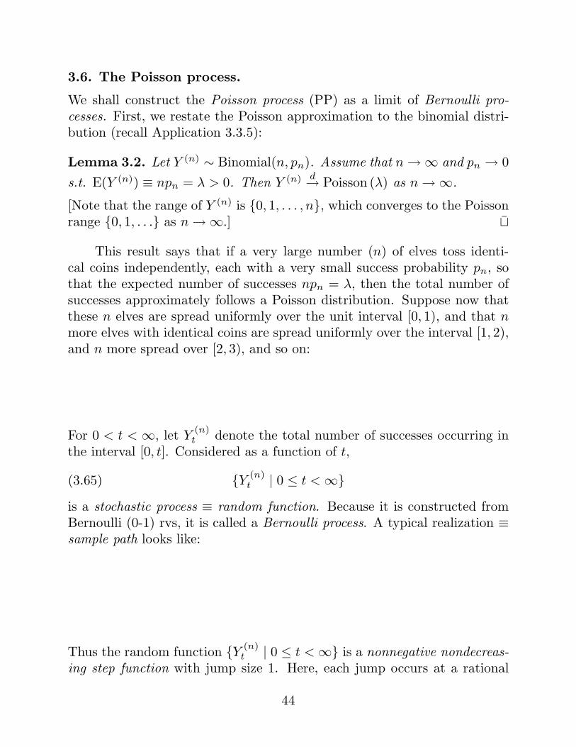
(3.65) Y (n)t | 0 ≤ t < ∞
is a stochastic process ≡ random function. Because it is constructed fromBernoulli (0-1) rvs, it is called a Bernoulli process. A typical realization ≡sample path looks like:
Thus the random function Y (n)t | 0 ≤ t < ∞ is a nonnegative nondecreas-
ing step function with jump size 1. Here, each jump occurs at a rational
44
point t = rn corresponding to the location point of a lucky elf who achieves
a success. Furthermore, because all the elves are probabilistically indepen-dent, for any 0 < t0 < t1 < t2 · · ·, the successive increments Y
(n)t1 − Y
(n)t0 ,
Y(n)t2 − Y
(n)t1 , ..., are mutually independent. Thus the Bernoulli process has
independent increments. Furthermore, for each increment
(3.66) Y(n)ti
− Y(n)ti−1
∼ Binomial((ti − ti−1)n, pn).
In particular,
(3.67) E[Y (n)ti
− Y(n)ti−1
] = (ti − ti−1)npn ≡ (ti − ti−1)λ,
which does not depend on n. In fact, here it depends only on λ and thelength of the interval (ti−1, ti).
Now let n → ∞ and let
(3.68) Yt | 0 ≤ t < ∞
be the limiting stochastic process. Since independence is preserved underlimits in distribution [cf. §10], for any 0 < t0 < t1 < t2 · · · the incrementsYt1 −Yt0 , Yt2 −Yt1 , ...of the limiting process remain mutually independent,and by Lemma 3.2 each increment
(3.69) Yti − Yti−1 ∼ Poisson((ti − ti−1)λ).
The process (3.68) is called a Poisson process (PP) with intensity λ. Itssample paths are again nonnegative nondecreasing step functions, againwith jump size 1. Such a process is called a point process because thesample path is completely determined by the locations of the jump pointsT1, T2, . . ., and these jump points can occur anywhere on (0,∞) (not justat rational points).
45

Note that (3.67) continues to hold for Yt:
(3.70) E[Y (ti) − Y (ti−1)] = (ti − ti−1)λ,
which again depends only on λ and the length of the interval (ti−1, ti).
[Such a process is called homogeneous. Non-homogeneous Poisson pro-cesses also can be defined, with λ replaced by an intensity function λ(t) ≥ 0.A non-homogeneous PP retains all the above properties of a homogeneousPP except that in (3.69) and (3.70), (ti − ti−1)λ is replaced by
∫ ti
ti−1λ(t)dt.
A non-homogeneous PP can be thought of as the limit of non-homogeneousBernoulli processes, where the success probabilities vary (continuously)along the sequence of elves.]
There is a duality between a (homogeneous) PP Yt | 0 ≤ t < ∞and sums of i.i.d. exponential random variables. This is (partially) seen asfollows. Let T1, T2, . . . be the times of the jumps of the PP.4
Proposition 3.1. T1, T2 − T1, T3 − T2, . . . are i.i.d. Exponential (λ) rvs.In particular, E(Ti − Ti−1) = 1
λ , which reflects the intuitive fact that theexpected waiting time to the next success is inversely proportional to theintensity rate λ.
Partial Proof. P [T1 > t] = P [no successes occur in (0, t] ] = P [Yt = 0]= e−λt, since Yt ∼ Poisson(λt). (The proof continues with Exercise 6.4.)
Note: Tk ∼ Gamma(k, λ), because the sum of i.i.d. exponential rvs has aGamma distribution. Since Tk > t = Yt ≤ k−1, this implies a relationbetween the cdfs of the Gamma and Poisson distributions: see CB Example3.3.1 and CB Exercise 3.19; also Ross Exercise 26, Ch. 4.]
In view of Proposition 3.1 and the fact that a PP is completely de-termined by the location of the jumps, a PP can be constructed froma sequence of i.i.d. Exponential (λ) rvs V1, V2, . . .: just define T1 = V1,
4 There must be infinitely many jumps in (0,∞). This follows from the Borel-
Cantelli Theorem, which says that if An is a sequence of independent events, then
P [infinitely many An occur] is 0 or 1 according to whether∑
P (An) is < ∞ or = ∞.
Now let An be the event that at least one success occurs in the interval (n − 1, n].
46
T2 = V1 + V2, T3 = V1 + V2 + X3, etc. Then T1, T2, T3, . . . determine thejump points of the PP, from which the entire sample path can be con-structed.
PPs arise in many applications, for example as a model for radioactivedecay over time. Here, an “elf” is an individual atom – each atom has atiny probability p of decaying (a ”success”) in unit time, but there are alarge number n of atoms. PPs also serve as models for the number of trafficaccidents over time (or location) on a busy freeway.
PPs can be extended in several ways: from homogeneous to non-homogeneous as mentioned above, and/or to processes indexed by morethan one parameter, e.g., t1, . . . , tk, so the process is written as
(3.71) Yt1,...,tk| t1 ≥ 0, . . . , tk ≥ 0.
This can be thought of as a limit of Bernoulli processes where the elves aredistributed in a k-dimensional space rather than along a 1-dimensional line.
The basic properties continue to hold, i.e., the number of successes occurringin non-overlapping regions are independent Poisson variates determined byan intensity function λ(t1, . . . , tk) ≥ 0, as follows: for any region R, thenumber of counts occurring in R has a Poisson distribution with parameter∫
Rλ(t1, . . . , tk)dt1, . . . , dtk. Examples of 2-dimensional random processes
that may be PPs include the spatial distribution of weeds in a field, of oredeposits in a region, or of erroneous pixels in a picture transmitted froma Mars orbiter. These are called “spatial” processes because the param-eters (t1, . . . , tk) determine a location, not because the process originatesfrom outer space. They are only “possibly” PP because the independenceproperty may not hold if spatial correlation is present.
47

The waiting-time paradox for a homogeneous Poisson Process.
Does it seem that your waiting time for a bus is usually longer than youhad expected? This can be explained by the memory-free property of theexponential distribution of the waiting times.
We will model the bus arrival times as the jump times T1 < T2 < · · · ofa homogeneous PP Yt on [0, ∞) with intensity λ. Thus the interarrivaltimes Vi ≡ Ti − Ti−1 (i ≥ 1, T0 ≡ 0) are i.i.d Exponential (λ) rvs and
(3.72) E(Vi) =1λ
, i ≥ 1.
Now suppose that you arrive at the bus stop at a fixed time t∗ > 0.Let the index j ≥ 1 be such that Tj−1 < t∗ < Tj (j ≥ 1), so Vj is the lengthof the interval that contains your arrival time. We expect from (3.72) that
E(Vj) =1λ
.(3.73)
Paradoxically, however [see figure],
E(Vj) = E(Tj − t∗) + E(t∗ − Tj−1) > E(Tj − t∗) =1λ
,(3.74)
since Tj − t∗ ∼ Expo (λ) by the memory-free property of the exponentialdistribution: if the next bus has not arrived by time t∗ then the additionalwaiting time to the next bus still has the Expo (λ) distribution. Thus youappear always to be unlucky to arrive at the bus stop during a longer-than-average interarrival time!
This paradox is resolved by noting that the index j is random, not fixed:it is the random index such that Vj includes t∗. The fact that this intervalincludes a prespecified point t∗ tends to make Vj larger than average: alarger interval is more likely to include t∗ than a shorter one! Thus it isnot so suprising that E(Vj) > 1
λ .
Exercise 3.4. A simpler example of this phenomenon can be seen asfollows. Let U1 and U2 be two random points chosen independently anduniformly on the (circumference of the) unit circle and let L1 and L2 bethe lengths of the two arcs thus obtained:
48
Thus, L1 + L2 = 2π and L1distn= L2 by symmetry, so
(3.76) E(L1) = E(L2) = π.
(i) Find the distributions of L1 and of L2.
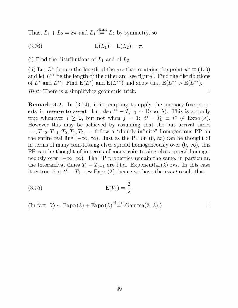
(ii) Let L∗ denote the length of the arc that contains the point u∗ ≡ (1, 0)and let L∗∗ be the length of the other arc [see figure]. Find the distributionsof L∗ and L∗∗. Find E(L∗) and E(L∗∗) and show that E(L∗) > E(L∗∗).Hint: There is a simplifying geometric trick.
Remark 3.2. In (3.74), it is tempting to apply the memory-free prop-erty in reverse to assert that also t∗ − Tj−1 ∼ Expo (λ). This is actuallytrue whenever j ≥ 2, but not when j = 1: t∗ − T0 ≡ t∗ ∼ Expo (λ).However this may be achieved by assuming that the bus arrival times. . . , T−2, T−1, T0, T1, T2, . . . follow a “doubly-infinite” homogeneous PP onthe entire real line (−∞, ∞). Just as the PP on (0, ∞) can be thought ofin terms of many coin-tossing elves spread homogeneously over (0, ∞), thisPP can be thought of in terms of many coin-tossing elves spread homoge-neously over (−∞, ∞). The PP properties remain the same, in particular,the interarrival times Ti − Ti−1 are i.i.d. Exponential (λ) rvs. In this caseit is true that t∗ − Tj−1 ∼ Expo (λ), hence we have the exact result that
(3.75) E(Vj) =2λ
.
(In fact, Vj ∼ Expo (λ) + Expo (λ) distn= Gamma(2, λ).)
49
4. Conditional Expectation and Conditional Distribution.
Let (X, Y ) be a bivariate rvtr with joint pmf (discrete case) or joint pdf(continuous case) f(x, y) . The conditional expectation of Y given X = x isdefined by
E[Y | X = x] =∑
y
yf(y|x), [discrete case](4.1)
E[Y | X = x] =∫
yf(y|x) dy, [continuous case](4.2)
provided that the sum or integral exists, where f(y|x) is given by (1.28) or(1.30). More generally, for any (measurable) function g(x, y),
E[g(X, Y ) | X = x] =∑
y
g(x, y)f(y|x), [discrete case](4.3)
E[g(X, Y ) | X = x] =∫
g(x, y)f(y|x) dy, [continuous case](4.4)
Note that (1.29) and (1.31) are special cases of (4.3) and (4.4), respectively,with g(x, y) = IB(y). For simplicity, we often omit “=x” when writing aconditional expectation or conditional probability.
Because f(·|x) is a bona fide pmf or pdf, conditional expectation enjoysall the properties of ordinary expectation, in particular, linearity:
(4.5) E[ag(X, Y ) + bh(X, Y ) | X] = aE[g(X, Y ) | X] + bE[h(X, Y ) | X].
The key iteration formula follows from (4.3), (1.28), (3.5) or (4.4),(1.30), (3.6):
(4.6) E[g(X, Y )] = E(E[g(X, Y ) | X]
). [verify]
As a special case (set g(x, y) = IC(x, y)), for any (measurable) event C,
(4.7) P [(X, Y ) ∈ C] = E(P [(X, Y ) ∈ C | X]
).
50
We now discuss the extension of these results to the two “mixed” cases.
(i) X is discrete and Y is continuous.
First, (4.6) and(4.7) continue to hold: (4.7) follows immediately fromthe law of total probability (1.54) [verify], then (4.6) follows since any (mea-surable) g can be approximated as g(x, y) ≈
∑ciICi(x, y). Thus, although
we cannot calculate P [(X, Y ) ∈ C] or E[g(X, Y )] directly since we do nothave a joint pmf or joint pdf, we can obtain them by the iteration formulasin (4.6) and (4.7). For this we can apply a formula analogous to (4.4), whichrequires us to determine f(y|x) as follows.
For any event B and any x s.t. P [X = x] > 0,
(4.8) P [Y ∈ B | X = x] ≡ P [Y ∈ B, X = x]P [X = x]
is well defined by the usual conditional probability formula (1.27). Thus wecan define
(4.9) f(y|x) =d
dyF (y|x) ≡ d
dyP [Y ≤ y | X = x].
Clearly f(y|x) ≥ 0 and∫
f(y|x)dy = 1 for each x s.t. P [X = x] > 0. Thusfor each such x, f(·|x) determines a bona fide pdf. Furthermore (cf. (1.31))
(4.10) P [Y ∈ B | X = x] =∫
B
f(y|x) dy ∀B.
so this f(y|x) does in fact represent the conditional distribution of Y givenX = x. [Using (4.9), verify (4.10) for B = (−∞, y], then extend to all B.]Now (4.10) can be extended by the approximation g(y) ≈
∑biIBi
(y) togive
(4.11) E[g(Y ) | X = x] =∫
g(y)f(y|x)dy
and similarly to give (4.4) (since E[g(X, Y ) | X = x] = E[g(x, Y ) | X = x].)
Note: In applications, f(y|x) is not found via (4.9) but instead is eitherspecified directly or else is found using f(x|y) and Bayes formula (4.14) –see Example 4.3.
51
(ii) X is continuous and Y is either discrete or continuous.
For any (measurable) event C and any x such that f(x) > 0, we definethe conditional probability
P [(X, Y ) ∈ C|X = x] = limδ↓0
P [(X, Y ) ∈ C | x ≤ X ≤ x + δ](4.12)
= limδ↓0
P [(X, Y ) ∈ C, x ≤ X ≤ x + δ]P [x ≤ X ≤ x + δ]
=1
f(x)limδ↓0
P [(X, Y ) ∈ C, x ≤ X ≤ x + δ]δ
≡ 1f(x)
d
dxP [(X, Y ) ∈ C, X ≤ x].(4.13)
Then the iteration formulas (4.6) and (4.7) continue to hold. For (4.7),
E(P [(X, Y ) ∈ C | X]
)=
∫ ∞
−∞
( d
dxP [(X, Y ) ∈ C, X ≤ x]
)dx [by (4.13)]
= P [(X, Y ) ∈ C].
Again (4.6) follows by the approximation g(x, y) ≈∑
ciICi(x, y).
In particular, if X is continuous and Y is discrete, then by (4.13),f(y|x) is given by
f(y|x) ≡ P [Y = y | X = x]
=1
f(x)d
dxP [Y = y, X ≤ x]
=1
f(x)d
dxP [X ≤ x | Y = y] · P [Y = y]
≡ f(x|y)f(y)f(x)
. [by (4.9)](4.14)
This is Bayes formula for pdfs in the mixed case, and extends (1.58).
Remark 4.1. By (4.14),
(4.15) f(y|x)f(x) = f(x|y)f(y),
52
even in the mixed cases where a joint pmf or pdf f(x, y) does not exist. Insuch cases, the joint distribution is specified either by specifying f(y|x) andf(x), or f(x|y) and f(y) – see Example 4.3.
Remark 4.2. If (X, Y ) is jointly continuous then we now have two defi-nitions of f(y|x): the “slicing” definition (1.30): f(y|x) = f(x,y)
f(x) , and thefollowing definition (4.16) obtained from (4.13):
f(y|x) ≡ d
dyF (y|x)
≡ d
dyP [Y ≤ y | X = x]
=d
dy
[ 1f(x)
d
dxP [Y ≤ y, X ≤ x]
][by (4.13)](4.16)
=1
f(x)∂2
∂x∂yF (x, y)
≡ f(x, y)f(x)
.
Thus the two definitions coincide in this case.
Remark 4.3. To illustrate the iteration formula (4.6), we obtain the fol-lowing useful result:
Cov(g(X), h(Y )) = E(g(X)h(Y )) − (Eg(X))(Eh(Y ))= E
(E[ g(X)h(Y ) | X]
)− (Eg(X))
[E(E[h(Y ) | X])
]= E
(g(X)E[h(Y ) | X]
)− (Eg(X))
[E(E[h(Y ) | X])
]= Cov(g(X), E[h(Y )|X]).(4.17)
Here we have used the Product Formula:
(4.18) E[g(X) h(Y ) | X] = g(X)E[h(Y ) | X].
Example 4.1. (Example 1.12 revisited.) Let (X, Y ) ∼ Uniform(D), whereD is the unit disk in R2. In (1.44) we saw that
Y |X ∼ Uniform(−
√1 − X2,
√1 − X2
),
53
which immediately implies E[Y |X] ≡ 0. Thus the iteration formula (4.6)and the covariance formula (4.17) yield, respectively,
E(Y ) = E(E[Y |X]
)= E(0) = 0,
Cov(X, Y ) = Cov(X, E[Y |X]) = Cov(X, 0) = 0,
which are also clear from considering the joint distribution of (X, Y ).
Example 4.2. Let (X, Y ) ∼Uniform(T ), where T is the triangle below, so
(4.19) f(x, y) =
2, 0 < x < 1, 0 < y < x;0, otherwise.
Thus
(4.20) f(x) = 2xI(0,1)(x),
hence
f(y|x) =
1x , 0 < y < x;0, otherwise.
That is,
(4.21) Y |X ∼ Uniform(0, X)
[verify from the figure by “slicing”], so
(4.22) E[Y | X] =X
2.
From (4.20) we have E(X) = 23 [verify], so the iteration formula gives
(4.23) E(Y ) = E(E[Y |X]
)= E
(X
2
)=
12· 23
=13.
Also from (4.17), (4.22), and the bilinearity of covariance,
Cov(X, Y ) =12
Cov(X, X) ≡ 12
Var(X).
But [verify from (4.20)]
(4.24) Var(X) = E(X2) − (E(X))2 =12−
(23
)2
=118
,
so Cov(X, Y ) = 136 > 0. Thus X and Y are positively correlated.
54
Example 4.3. (A “mixed” joint distribution: Binomial-Uniform). Sup-pose that the joint distribution of (X, Y ) is specified by the conditionaldistribution of X|Y and the marginal distribution of Y (≡ “p”) as follows:
(4.25)X|Y ∼ Binomial(n, Y ), (discrete)
Y ∼ Uniform (0, 1), (continuous)so
(4.26)f(x|y) =
(n
x
)yx(1 − y)n−x, x = 0, . . . , n,
f(y) = 1, 0 < y < 1.
Here, X is discrete and Y is continuous, and their joint range is
(4.25) ΩX,Y = ΩX × ΩY = 0, 1, . . . , n × (0, 1).
However, (4.25) shows that X ⊥⊥ Y , since the conditional distribution ofX|Y varies with Y . In particular,
(4.28) E[X | Y ] = nY.
Suppose that only X is observed and we wish to estimate Y by E[Y |X].For this we first need to find f(y|x) via Bayes formula (4.14). First,
f(x) ≡ P [X = x] = E(P [X = x | Y ]
)= E
[(n
x
)Y x(1 − Y )n−x
]=
(n
x
) ∫ 1
0
yx(1 − y)n−xdy
=(
n
x
) ∫ 1
0
y(x+1)−1(1 − y)(n−x+1)−1dy
=(
n
x
)Γ(x + 1)Γ(n − x + 1)
Γ(n + 2)[see (1.10)]
=n!
x!(n − x)!· x!(n − x)!
(n + 1)!
=1
n + 1, x = 0, 1, . . . , n.(4.29)
55
This shows that, marginally, X has the discrete uniform distribution overthe integers 0, . . . , n. Then from (4.14),
f(y|x) =
(nx
)yx(1 − y)n−x · 1
1n+1
=(n + 1)!
x!(n − x)!yx(1 − y)n−x
≡ Γ(n + 2)Γ(x + 1)Γ(n − x + 1)
yx(1 − y)n−x, 0 < y < 1.(4.30)
Thus, the conditional (≡ posterior) distribution of Y given X is
(4.31) Y |X ∼ Beta (X + 1, n − X + 1),
so the posterior ≡ Bayes estimator of Y |X is given by
E[Y | X] =∫ 1
0
y ·[ Γ(n + 2)Γ(X + 1)Γ(n − X + 1)
yX(1 − y)n−X]
=Γ(n + 2)
Γ(X + 1)Γ(n − X + 1)
∫ 1
0
y(X+2)−1(1 − y)(n−X+1)−1
=Γ(n + 2)
Γ(X + 1)Γ(n − X + 1)· Γ(X + 2)Γ(n − X + 1)
Γ(n + 3)
=(n + 1)!(X + 1)!
X!(n + 2)!
=X + 1n + 2
. (4.32)
Remark 4.4. If we observe X = n successes (so no failures), then the Bayesestimator is n+1
n+2 , not 1. In general, the Bayes estimator can be written as
(4.33)X + 1n + 2
=n
n + 2
(X
n
)+
2n + 2
(12
),
which is a convex combination of the usual estimate Xn and the a priori
estimate 12 ≡ E(Y ). Thus the Bayes estimator adjusts the usual estimate
to reflect the a priori assumption that Y ∼ Uniform(0, 1). Note, however,that the weight n
n+2 assigned to Xn increases to 1 as the sample size n → ∞,
i.e., the prior information becomes less influential as n → ∞. (See §16.)
56
Example 4.4: Borel’s Paradox. (This example shows the need forthe limit operation (4.12) in the definition of the conditional probabilityP [(X, Y ) ∈ C|X = x] when X is continuous:)
As in Examples 1.12 and 4.1, let (X, Y ) be uniformly distributed overthe unit disk D in R2 and consider the conditional distribution of |Y | givenX = 0. The “slicing” formula (1.30) applied to f(x, y) ≡ ID(x, y) gives
Y∣∣ X = 0 ∼ Uniform(−1, 1),
so [verify]
(4.34) |Y |∣∣ X = 0 ∼ Uniform(0, 1).
However, if we represent (X, Y ) in terms of polar coordinates (R, Θ) as inExample 1.12, then the event X = 0 is equivalent to Θ = π
2 or 3π2 ,
while under this event, |Y | = R. However, we know that R ⊥⊥ Θ andf(r) = 2rI(0,1)(r) (recall (1.45) and (1.46a)), hence the “slicing” formula(1.30) applied to f(r, θ) ≡ f(r)f(θ) shows that
(4.35) R∣∣∣
Θ =π
2or
3π
2
∼ f(r) = Uniform(0, 1).
Since the left sides of (4.34) and (4.35) appear identical, this yieldsBorel’s Paradox. The paradox is resolved by noting that, according to(4.12), conditioning on X is not equivalent to conditioning on Θ:
Conditioning on X = 0 Conditioning on
Θ = π2 or 3π
2
57
5. Correlation, Prediction, and Regression.
5.1. Correlation. The covariance Cov(X, Y ) indicates the nature (posi-tive or negative) of the linear relationship (if any) between X and Y , butdoes not indicate the strength, or exactness, of this relationship. The Pear-son correlation coefficient
(5.1) Cor(X, Y ) =Cov(X, Y )√VarX
√VarY
≡ ρX,Y ,
the standardized version of Cov(X, Y ), does serve this purpose.
Properties:
(a) Cor(X, Y ) = Cor(Y, X).
(b) location-scale: Cor(aX + b, cY + d) = sgn(ac) · Cor(X, Y ).
(c) −1 ≤ ρX,Y ≤ 1. Equality holds (ρX,Y = ±1) iff Y = aX + b for somea, b, i.e., iff X and Y are perfectly linearly related.
Proof. Let U = X − EX, V = Y − EY , and
g(t) = E[(tU + V )2
]= t2E(U2) + 2tE(UV ) + E(V 2).
Since this quadratic function is always ≥ 0, its discriminant is ≤ 0, i.e.
(5.2)[E(UV )
]2 ≤ E(U2) · E(V 2),
so
(5.3)[Cov(X, Y )
]2 ≤ VarX · VarY,
which is equivalent to ρ2X,Y ≤ 1. [(5.2) is the Cauchy-Schwartz Inequality.]
Next, equality holds in (5.2) iff the discriminant of g is 0, so g(t0) = 0for some t0. But g(t0) = E
[(t0U + V )2
], hence t0U + V ≡ 0, so V must be
exactly a linear function of U , i.e., Y is exactly a linear function of X.
Property (c) suggests that the closer ρ2X,Y is to 1, the closer the rela-
tionship between X and Y is to exactly linear. (Also see (5.22).)
58

5.2. Mean-square error prediction (general regression).
For any rv Y s.t. E(Y 2) < ∞ and any −∞ < c < ∞,
E[(Y − c)2
]= E
([(Y − EY ) + (EY − c)
]2)= E
[(Y − EY )2
]+ (EY − c)2 + 2(EY − c)E(Y − EY )
= VarY + (EY − c)2.(5.4)
Thus c = EY is the best predictor of Y w.r.to mean-square error (MSE) inthe absence of any other information, and the minimum MSE is
(5.5) min−∞<c<∞
E[(Y − c)2
]= VarY.
Now consider a bivariate rvtr (X, Y ) with E(Y 2) < ∞. How can webest use the information in X to obtain a better predictor g(X) of Y thanEY ? That is, what function g(X) minimizes the MSE
(5.6) E[(Y − g(X))2] = E(E
[(Y − g(X))2 | X
])?
But this follows immediately if we hold X fixed and in (5.4) and (5.5),replace the marginal distribution of Y by the conditional distribution of Ygiven X and replace c by g(X):
E[(Y − g(X))2 | X
]= Var[Y |X] +
(E[Y |X] − g(X)
)2;(5.7)
min−∞<g(X)<∞
E[(Y − g(X))2 | X
]= Var[Y |X].(5.8)
Thus g(X) = E[Y |X] is the best predictor of Y based on X, and from (5.6)the minimum (unconditional) MSE is
(5.9) ming(X)
E[(Y − g(X))2
]= E
(Var[Y |X]
).
The best predictor E[Y |X] is often called the regression function [ex-plain] of Y on X. The prediction error Y − E[Y |X] is called the residual.The basic decomposition formula for the prediction of Y by X is:
(5.10) Y = E[Y |X] +(Y − E[Y |X]
)≡ best predictor + residual.
Note that: E(best predictor)=EY and E(residual)=0. [verify]
59
Proposition 5.1. (Variance decomposition). The variance of Y can bedecomposed as follows:
VarY = Var(E[Y |X]
)+ E
(Var [Y |X]
)(5.11)
= Var(best predictor) + Var(residual).
Equivalently, the best predictor and residual are uncorrelated:
(5.12) Cov(E[Y |X], Y − E[Y |X]
)= 0.
Proof. Set g(X) = EY in (5.7) to obtain
E[(Y − EY )2 | X
]= Var[Y |X] +
(E[Y |X] − EY
)2.
Take expectations w.r.to X to obtain (5.11) (since E(E[Y |X]) = EY ). Now
Var(Y − E[Y |X]
)= E
[(Y − E[Y |X]
)2] [verify]
= E(E
[(Y − E[Y |X]
)2] | X)
= E(Var [Y |X]
), [verify](5.13)
so (5.12) follows from (3.13), (5.11), and (5.13).
Exercise 5.1. Prove (5.12) directly from (3.11) or (3.12) by conditioningon X and using the iteration formula.
Remark 5.1. Consider a rvtr (X1, . . . , Xk, Y ) with E(Y 2) < ∞. Thenthe best predictor g(X1, . . . , Xk) of Y | (X1, . . . , Xk) is E[Y | X1, . . . , Xk].All of the results above remain valid with X replaced by X1, . . . , Xk. Forexample, (5.9) becomes
(5.14) ming(X1,...,Xk)
E[(Y − g(X1, . . . , Xk))2
]= E
(Var[Y |X1, . . . , Xk]
),
which implies that
(5.15) E(Var[Y |X1, . . . , Xk]
)≤ · · · ≤ E
(Var[Y |X1]
)≤ VarY.
60
5.3. Linear prediction (≡ linear regression).
In practice, the best predictor ≡ regression function E[Y |X] is unavailable,since to find it would require knowing the entire joint distribution of (X, Y ).As a first step, we might ask to find the linear prediction function g(X) =a + bX that minimizes the MSE
(5.16) E([Y − (a + bX)]2
).
First hold b fixed. From (5.4) with Y replaced by Y − bX, the MSE isminimized when
a = a(b) = E(Y − bX) = E(Y ) − bE(X),(5.17)
mina
E[(Y − (a + bX)]2
)= E
([Y − EY ] − b[X − EX]
)2so
= VarY − 2b Cov(X, Y ) + b2VarX.
This is a quadratic in b and is minimized when
b =Cov(X, Y )
VarX,(5.18)
mina,b
E([Y − (a + bX)]2
)= VarY − 2
[Cov(X, Y )]2
VarX+
[Cov(X, Y )]2
VarXso
= VarY − [Cov(X, Y )]2
VarX.(5.19)
Thus from (5.17) and (5.18), the best linear predictor (BLP) of Y |X is
a(b) + bX =[EY −
(Cov(X, Y )VarX
)EX
]+
[Cov(X, Y )VarX
]X
= EY +(Cov(X, Y )
VarX
)[X − EX].(5.20)
≡ µY + ρX,Y
(σY
σX
)(X − µX),(5.21)
where µX = EX, µY = EY , σX = sd(X), σY = sd(Y ). From (5.19) theMSE of the BLP a + bX is
E([Y − (a + bX)]2
)= σ2
Y −ρ2
X,Y σ2Xσ2
Y
σ2X
= (1 − ρ2X,Y )σ2
Y ,(5.22)
61
The error of linear prediction Y − (a+ bX) is again called the residual.[See scatter plots.] The basic decomposition formula for linear prediction is:
Y = (a + bX) + [Y − (a + bX)](5.23)≡ best linear predictor + residual.
Again: E(best linear predictor)=EY and E(residual)=0. [verify]
Proposition 5.2. (Linear variance decomposition). The variance of Y canbe decomposed as follows:
VarY ≡ ρ2X,Y σ2
Y + (1 − ρ2X,Y )σ2
Y
≡ ρ2X,Y
(σ2Y
σ2X
)σ2
X + (1 − ρ2X,Y )σ2
Y(5.24)
= Var(best linear predictor) + Var(residual).
Equivalently, the best linear predictor and residual are uncorrelated:
(5.25) Cov(a + bX, Y − (a + bX)
)= 0.
Proof. From (5.21) and (5.22) [verify],
Var(BLP) = ρ2X,Y
(σ2Y
σ2X
)σ2
X ,(5.26)
Var(residual) = (1 − ρ2X,Y )σ2
Y ,(5.27)
so (5.24) holds. Then (5.25) follows from (3.13) and (5.24).
Exercise 5.2. Prove (5.25) directly using the bilinearity of covariance.
Remark 5.2. Note that (5.22) gives another proof that −1 ≤ ρX,Y ≤ 1,or equivalently, ρ2
X,Y ≤ 1. Also, it follows from (5.24) that ρ2X,Y , not
|ρX,Y |, expresses the strength of the linear relationship between X and Y :if ρ2
X,Y = 1 then there is an exact linear relationship, while if ρ2X,Y = 0
there is no overall linear relationship and the BLP reduces to the constantEY . Note that it is possible that ρ2
X,Y < 1 even if there is an exact non-linear relationship between X and Y ; for example if Y = eX exactly. (Here,however, there is a perfect linear relationship between log Y and X.)
62

FPP scatter plot 1
63

FPP scatter plot 2
64

Remark 5.3. Suppose we know that E[Y |X] is a linear function, i.e.,E[Y |X] = c + dX. (This holds in multinomial and multivariate normaldistributions – see §7.5 and §8.3). Then necessarily E[Y |X] = a + bX,i.e., the best general predictor must coincide with the best linear predictor[why?]. In this case, all the results in §5.2 reduce to those in §5.3.
Exercise 5.3. Prove or disprove: E[Y |X] is linear ⇒ E[X|Y ] is linear.
Example 5.1. (Another Bayesian example.) Let X = height of father,Y = height of son. Suppose that the joint distribution of (X, Y ) is specifiedby the conditional distribution of Y |X and the marginal distribution of Xas follows:
(5.28)Y |X ∼ Normal(X, τ2),
X ∼ Normal (µ, σ2),
so
(5.29)f(y|x) =
1√2πτ
e−(y−x)2
2τ2 ,
f(x) =1√2πσ
e−(x−µ)2
2σ2 .
Suppose that we observe a son’s height Y and want to estimate ( ≡ predict)his father’s height X using E[X|Y ]. For this we find f(x|y) via Bayes’formula (4.14):
f(x|y) =f(y|x)f(x)
f(y)
=constf(y)
· e−h(x),
where
(5.30) h(x) ≡ (y − x)2
2τ2+
(x − µ)2
2σ2
is a quadratic in x with leading term
(5.31)x2
2
( 1τ2
+1σ2
)≡ x2
2
( 1γ2
).
65
Since h(x) is minimized when
h′(x) ≡ x − y
τ2+
x − µ
σ2= 0,
i.e., when
(5.32) x =yτ2 + µ
σ2
1τ2 + 1
σ2
≡ c(y),
it follows that
h(x) =(x − c(y))2
2γ2+ d(y),
where d(y) does not involve x. Thus f(x|y) must have the following form:
f(x|y) =const · e−d(y)
f(y)· e−
(x−c(y))2
2γ2 .
However, since f(x|y) must be a pdf in x for each fixed y, we conclude that
f(x|y) =1√2πγ
e− (x−c(y))2
2γ2 .
(Note that it was not necessary to find f(y)!) Thus the conditional (≡posterior) distribution of X given Y is
X|Y ∼ N(c(Y ), γ2
)≡ N
(Yτ2 + µ
σ2
1τ2 + 1
σ2
,1
1τ2 + 1
σ2
),(5.33)
so the best estimator ≡ predictor of X|Y is
(5.34) E[X|Y ] =Yτ2 + µ
σ2
1τ2 + 1
σ2
,
a linear function of Y . In fact, this is again a convex combination of the“unbiased” estimate Y (recall (5.30) and the a priori estimate µ ≡ E(X).
66
Note that the weights assigned to Y and µ are inversely proportional to τ2
and σ2, respectively [interpret!]. Also, since E[X|Y ] is a linear function ofY , (5.34) is also the best linear predictor of X|Y (recall Remark 5.3).
How good is E[X|Y ]? From (5.13) (with X and Y interchanged), itsMSE is given by
E[(X − E[X|Y ])2
]= Var
(X − E[X|Y ]
)= E
(Var[X|Y ]
)=
11τ2 + 1
σ2
(5.35)
≈
0, if σ2 ≈ 0 (i.e., if prior info very good);τ2, if σ2 ≈ ∞ (i.e., if prior info not good).
The result (5.35) can also be derived in terms of ρX,Y . First,
VarX = σ2; [by (5.28)]VarY = Var
(E[Y |X]
)+ E
(Var [Y |X]
)[by (5.11)]
= VarX + E(τ2) [by (5.28)]= σ2 + τ2;
Cov(X, Y ) = Cov(X, E[Y |X]) [by (4.17)]= Cov(X, X)= σ2.
Thus
(5.36) 1 − ρ2X,Y = 1 − σ2
σ2 + τ2=
τ2
σ2 + τ2,
so by (5.22) (with X and Y interchanged), the MSE of E[X|Y ] is given by
(5.37) (1 − ρ2X,Y ) σ2 =
τ2σ2
σ2 + τ2,
which agrees with (5.35).
67
Remark 5.4. Consider a rvtr (X1, . . . , Xk, Y ) with E(Y 2) < ∞. Allthe above results remain valid but matrix notation is required – see §8.2.For example, the best linear predictor g(Xk) ≡ a + btXk of Y based onXk ≡ (X1, . . . , Xk)t is given by (compare to (5.20) and (8.76))
(5.38) a + btXk = EY + Cov(Y,Xk)[Cov(Xk)]−1(Xk − E(Xk)),
while (5.24)-(5.27) remain valid if ρ2X,Y is replaced by the multiple correla-
tion coefficient
(5.39) ρ2Xk,Y ≡ Cov(Y,Xk)[Cov(Xk)]−1Cov(Xk, Y )(VarY )−1.
In particular, the extension of (5.22) implies that
(5.40) 1 ≥ ρ2Xk,Y ≥ · · · ≥ ρ2
X1,Y ≥ 0.
Remark 5.5. In practice, the population quantities µX , µY , σ2X , σ2
Y ,and ρX,Y that appear in the BLP a + bX (5.21) are unknown, so must beestimated from a sample (X1, Y1), . . . , (Xn, Yn). The usual estimators are:
(5.41)
µX = Xn, µY = Yn,
σ2X =
1n − 1
n∑i=1
(Xi − Xn)2, σ2Y =
1n − 1
n∑i=1
(Yi − Yn)2,
ρX,Y =∑n
i=1(Xi − Xn)(Yi − Yn)√∑ni=1(Xi − Xn)2
√∑ni=1(Yi − Yn)2
.
When (X, Y ) has a bivariate normal distribution these estimators are theMLEs (CB Exercise 7.18), hence asymptotically optimal by Theorem 14.20.
Remark 5.6. If a linear predictor is not appropriate, i.e., if it is not thecase that Y ≈ a + bX (+ error), it may be the case that a tranformationwill convert the non-linear relation into a linear one. For example,
Y ≈ aebX ⇒ Y ′ ≡ log Y ≈ (log a) + bX(5.42)Y ≈ aXb ⇒ Y ′ ≡ log Y ≈ (log a) + b(log X),(5.43)
Y ≈ a + bX2 ⇒ Y ′ ≡ Y ≈ a + b(X2).(5.44)
68
(Of course, one must assume that the error in Y ′, not Y , is additive.) Note: The examples (5.42) – (5.44) emphasize that the “linearity” in a “lin-ear model” comes from the (approximate) linear dependence of the responseY on the unknown parameters a, b, log a, etc., not on X! (See §8.5.)
5.4. Covariance and Regression.
Proposition 5.3. If E[Y |X] is a strictly increasing function of X, thenCov(X, Y ) > 0.
Proof. This is an immediate consequence of (4.17) and the following lemma.
Lemma 5.1. (Chebyshev’s Other Inequality) If X is a non-degeneraterv and g(X) and h(X) are both strictly increasing in X, then
(5.45) Cov(g(X), h(X)) > 0.
Proof. Let Y be another rv with the same distribution as X and indepen-dent of X. Then
[g(X) − g(Y )][h(X) − h(Y )] ≥ 0,
with strict inequality whenever X = Y , which occurs with positive proba-bility since X and Y are independent and non-degenerate [verify]. Thus
0 < E([g(X) − g(Y )][h(X) − h(Y )]
)= E[g(X)h(X)] − E[g(X)h(Y )] − E[g(Y )h(X)] + E[g(Y )h(Y )]
= 2(E[g(X)h(X)] − E[g(X)]E[h(X)]
),
since X and Y are i.i.d., which yields (5.45).
69
6. Transforming Continuous Multivariate Distributions.
6.1. Two functions of two random variables.
Let (X, Y ) be a continuous random vector with joint pdf fX,Y (x, y) andconsider a transformation (X, Y ) → (U, V ), where
(6.1) U = u(X, Y ), V = v(X, Y ).
The pdf fU,V (u, v) is obtained by differentiating the joint cdf FU,V (u, v):
fU,V (u, v) =∂2
∂u∂vFU,V (u, v)
=∂2
∂u∂vP [U ≤ u, V ≤ v]
=∂2
∂u∂v
∫∫R(u,v)
fX,Y (x, y)dx dy,(6.2)
where R(u, v) is the region (x, y) | u(x, y) ≤ u, v(x, y) ≤ v. If the doubleintegral can be evaluated5 explicitly, then the derivatives can be taken toobtain fU,V (u, v). Three examples of this method6 are now presented.
Example 6.1. Let (X, Y ) be uniformly distributed on the unit square; set
(6.3) U = max(X, Y ), V = min(X, Y ).
In Example 2.5 we found the marginal pdfs of U and V separately. Herewe find the joint pdf of (U, V ) by using (6.2).
First specify the range of (U, V ): this is just the triangle
T ≡ (u, v) | 0 < u < 1, 0 < v < u
from Example 4.2. Then for (u, v) ∈ T ,
5 If the mapping (X, Y ) → (U, V ) given by (6.1) is differentiable and 1-1, then the
integral in (6.2) need not be evaluated – instead, fU,V (u, v) can be obtained by simply
multiplying fX,Y (x, y) by the Jacobian – see §6.2.6 Another example was given earlier – see (1.45).
70
FU,V (u, v) = P [U ≤ u] − P [U ≤ u, V > v]= P [X ≤ u, Y ≤ u] − P [v < X ≤ u, v < Y ≤ u]= u2 − (u − v)2, [by independence − verify]
fU,V (u, v) = 2IT (u, v),(6.4)
which is the same as (4.19). Thus (U, V ) is uniformly distributed on T .
Note:E(UV ) = E(XY ) = (EX)(EY ) =
14,
E(U + V ) = E(X + Y ) = 1,
E(V ) =∫ 1
0
[1 − FV (v)
]dv =
∫ 1
0
(1 − v)2dv =13,
so E(U) = 23 , hence (recall Example 4.2)
Cov(U, V ) =14− (EU)(EV ) =
14−
(23
) (13
)=
136
.
Example 6.2. Let X, Y be i.i.d. Exponential(1) rvs and set
(6.5) V = min(X, Y ), Z = |X − Y | ≡ max(X, Y ) − min(X, Y ).
In Example 2.6 we found the marginal pdfs of V and Z separately. Herewe find the joint pdf of (V, Z) via (6.2).
The range of (V, Z) is (0,∞) × (0,∞). For 0 < v < ∞, 0 < z < ∞,
P [V ≤ v, Z ≤ z] = P [Z ≤ z] − P [V > v, Z ≤ z],
P [V > v, Z ≤ z] = P [X > v, Y > v, |X − Y | ≤ z]= P [(X, Y ) in shaded region]= 2P [(X, Y ) in half of region](6.6)= 2P [X > v, X ≤ Y ≤ X + z]
71
= 2∫ ∞
v
e−x( ∫ x+z
x
e−ydy)dx
= 2∫ ∞
v
e−x(e−x − e−x−z
)dx
= 2(1 − e−z
) ∫ ∞
v
e−2xdx
= e−2v(1 − e−z
),
where (6.6) follows by symmetry: (X, Y ) ∼ (Y, X). Therefore
fV,Z(v, z) = − ∂2
∂v∂z
[e−2v
(1 − e−z
)]=
(2e−2v
)(e−z
)(6.7)
= fV (v) fZ(z), [recall (2.17), (2.20)]
so V and Z are independent, with
V ∼ Exponential(2), Z ∼ Exponential(1).
Interpretation: Suppose that X, Y represent the lifetimes of two lightbulbs.Thus, V ≡ min(X, Y ) is the time to the first burnout (either X or Y ). Oncethe first burnount occurs, the time to the second burnout has the originalexponential distribution Expo(1), not Expo(2). This is another memory-free property of the exponential distribution. It is stronger in that it showsthat the process renews itself at the random time V . (The first memory-freeproperty concerned any fixed renewal time t.)
Exercise 6.1**. (Converse of Example 6.2: a second characterizationof the exponential distribution (compare to Exercise 1.2).) Let X, Y benonnegative i.i.d. rvs with common pdf f on (0,∞). Show that if V ≡min(X, Y ) and Z ≡ |X − Y | are independent, then X and Y must beexponential rvs, i.e., f(x) = λe−λx for some λ > 0.Hint: follow the approach of Example 6.2. For simplicity, you may assumethat f is strictly positive and continuous.
Example 6.3. Again let X, Y be i.i.d. Exponential(1) rvs and set
(6.8) U = X + Y, W =X
X + Y.
72
In Example 2.6 we found the marginal pdfs of U and W separately. Herewe find the joint pdf of (U, W ) via (6.2).
The range of (U, W ) is (0,∞) × (0, 1). For 0 < u < ∞, 0 < w < 1,
P [U ≤ u, W ≤ w] = P [X + Y ≤ u, X ≤ w(X + Y )]
= E(
P[Y ≤ u − X, Y ≥
(1 − w
w
)X
∣∣ X])
=∫ uw
0
e−x( ∫ u−x(
1−ww
)x
e−ydy)dx
=∫ uw
0
(e−
xw − e−u
)dx
= [1 − e−u − ue−u] · w.(6.9)
Therefore
fU,W (u, w) =∂2
∂u∂w[1 − e−u − ue−u] · w
=(ue−u
)· 1(6.10)
= fU (u) fW (w), [recall (2.16), (2.21)]
so U and W are independent, with
U ∼ Gamma(2, 1), W ∼ Uniform(0, 1).
Interpretation: As noted in Example 2.6, (6.9) and (6.10) can be viewed asa “backward” memory-free property of the exponential distribution: givenX+Y , the location of X is uniformly distributed over the interval (0, X+Y ),i.e., over the “past”.
73
6.2. The Jacobian method.
Let A, B be open sets in Rn and
(6.11)T : A → B
x ≡ (x1, . . . , xn) → y ≡ (y1, . . . , yn)
a smooth bijective (1-1 and onto) mapping (≡ diffeomorphism). The Jaco-bian matrix of this mapping is given by
(6.12) JT (x) ≡(∂y
∂x
):=
∂y1∂x1
· · · ∂yn
∂x1
......
∂y1∂xn
· · · ∂yn
∂xn
;
the Jacobian of the mapping is given by
|JT (x)| ≡∣∣∣∂y
∂x
∣∣∣ := |det(∂y
∂x
)| ≥ 0.
Theorem 6.1. (Substitution formula for multiple integrals.) Let A, B beopen sets in Rn and T : A → B a diffeomorphism such that |JT (x)| > 0 for“a.e.” x. Let f be a real-valued integrable function on A. Then
(6.13)∫
A
f(x)dx =∫
B=T (A)
f(T−1(y))∣∣∣∂x
∂y
∣∣∣ dy. [explain]
[See (6.16) for the relation between∣∣∂x∂y
∣∣ and∣∣ ∂y∂x
∣∣.]Corollary 6.2. Let X be a random vector (rvtr) with pdf fX(x) (wrtoLebesgue measure) on Rn. Suppose that A := x | fX(x) > 0 is open andthat T : A → B is a diffeomorphism with JT (x) > 0 a.e. Then the pdf ofY := T (X) is given by
(6.14) fY (y) = fX(T−1(y)) ·∣∣∣∂x
∂y
∣∣∣ · IB(y).
74
Proof. For any (measurable) set C ⊆ Rn,
P [Y ∈ C] =P [X ∈ T−1(C)]
=∫
T−1(C)
fX(x)dx
=∫
C
f(T−1(y))∣∣∣∂x
∂y
∣∣∣dy,
which confirms (6.14) [Why?]
The calculation of Jacobians can be simplified by application of thefollowing rules.
Chain Rule: Suppose that x → y and y → z are diffeomorphisms. Thenx → z is a diffeomorphism and
(6.15)∣∣∣∂z
∂x
∣∣∣ =∣∣∣∂z
∂y
∣∣∣y=y(x)
·∣∣∣∂y
∂x
∣∣∣.[This follows from the chain rule for partial derivatives:
∂zi(y1(x1, . . . , xn), . . . , yn(x1, . . . , xn))∂xj
=∑
k
∂zi
∂yk
∂yk
∂xj=
[(∂z
∂y
)(∂y
∂x
)]ij
.
Therefore(
∂z∂x
)=
(∂z∂y
)(∂y∂x
); now take determinants.]
Inverse Rule: Suppose that x → y is a diffeomorphism. Then∣∣∣∂x
∂y
∣∣∣y=y(x)
=∣∣∣∂y
∂x
∣∣∣−1
.
[Set z = x in (6.15).] Reversing the roles of x and y we obtain
(6.16)∣∣∣∂y
∂x
∣∣∣x=x(y)
=∣∣∣∂x
∂y
∣∣∣−1
.
Combination Rule: Suppose that x → u and y → v are (unrelated) diffeo-morphisms. Then
(6.17)∣∣∣∂(u, v)∂(x, y)
∣∣∣ =∣∣∣∂u
∂x
∣∣∣ · ∣∣∣∂v
∂y
∣∣∣.75
[The Jacobian matrix is given by
(∂(u, v)∂(x, y)
)=
( ∂u∂x 00 ∂v
∂y
). ]
Extended Combination Rule: Suppose that (u, v) → (x, y) is a diffeomor-phism of the form u = u(x), v = v(x, y). Then (6.17) remains valid.
[The Jacobian matrix is given by
(∂(u, v)∂(x, y)
)=
( ∂u∂x
∂v∂x
0 ∂v∂y
). ]
Jacobians of linear mappings. Let A : p × p and B : n × n be nonsingularmatrices and c a nonzero scalar (A, B, L, M, U, V, c fixed.) Then:
(a) vectors: y = cx, x, y : p × 1:∣∣ ∂y∂x
∣∣ = |c|p. [combination rule]
(b) matrices: Y = cX, X, Y : p × n:∣∣ ∂Y∂X
∣∣ = |c|pn. [comb. rule]
(c) symmetric matrices: Y = cX, X, Y : p× p, symmetric:∣∣ ∂Y∂X
∣∣ = |c| p(p+1)2 .
[comb. rule](d) vectors: y = Ax, x, y : p × 1, A : p × p:
∣∣ ∂y∂x
∣∣ = |det A|. [verify]
(e) matrices: Y = AX, X, Y : p × n:∣∣ ∂Y∂X
∣∣ = |det A|n. [comb. rule]
Y = XB, X, Y : p × n:∣∣ ∂Y∂X
∣∣ = |det B|p. [comb. rule]
Y = AXB, X, Y : p × n:∣∣ ∂Y∂X
∣∣ = |det A|n|det B|p. [chainrule]
Example 6.4. The Gamma(α, λ) distribution with shape parameter α > 0and intensity parameter λ > 0 has pdf
(6.18) g(x;α, λ) =λα
Γ(α)xα−1e−λxI(0,∞)(x).
Let X ∼ Gamma(α, λ) and Y ∼ Gamma(β, λ) be independent Gammarandom variables with the same scale parameter and define
(6.19) U = X + Y, W =X
X + Y.
76
Find the joint pdf of (U, W ), find the marginal pdfs of U and W , and showthat U and W are independent. (This extends Example 6.3.)
Solution. The ranges of (X, Y ) and (U, W ) are
A : = (x, y) | x > 0, y > 0 ≡ (0,∞) × (0,∞),B : = (u, w) | u > 0, 0 < w < 1 ≡ (0,∞) × (0, 1),
respectively. Notice that both A and B are Cartesian product sets. Thetransformation
(6.20)T : A → B
(x, y) → (x + y, x/(x + y))
is bijective, with inverse given by
(6.21)T−1 : B → A
(u, w) → (uw, u(1 − w)).
Thus T−1 is continuously differentiable and bijective, and its Jacobian isgiven by [verify!]
(6.22)∣∣∣ ∂(x, y)∂(u, w)
∣∣∣ =∣∣∣ ∂(uw)
∂u∂(uw)
∂w∂(u(1−w))
∂u∂(u(1−w))
∂w
∣∣∣ =∣∣∣ w u1 − w −u
∣∣∣ = u.
Because
(6.23) fX,Y (x, y) =λα+β
Γ(α)Γ(β)xα−1e−λxyβ−1e−λyIA(x, y),
it follows from (6.14) that
fU,W (u, w) =λα+β
Γ(α)Γ(β)(uw)α−1e−λuw(u(1 − w))β−1e−λu(1−w) · u · IB(u, w)
=λα+βuα+β−1e−λu
Γ(α + β)I(0,∞)(u) · Γ(α + β)
Γ(α)Γ(β)wα−1(1 − w)β−1I(0,1)(w)(6.24)
≡fU (u) · fW (w).
77
Thus U ⊥⊥ W , U ∼ Gamma(α + β, λ), W ∼ Beta(α, β).
Remark 6.1. (The converse of Example 6.4 – a characterization of theGamma distribution.) The Gamma family is the only family of distribu-tions on (0,∞) with the property that X + Y and X
X+Y are independent.[References: Hogg (1951 Ann. Math. Statist.); Lukacs (1955 Ann. Math.Statist.); G. Marsaglia (Festschrift for I. Olkin); Kagan, Linnik, Rao (book).
Remark 6.2. Let U and W be independent with U ∼ Gamma(α+β, λ) andW ∼ Beta(α, β). It follows from Example 6.4 that UW ∼ Gamma(α, λ),U(1 − W ) ∼ Gamma(β, λ), and UW ⊥⊥ U(1 − W ) [verify].
Exercise 6.2. Let X, Y, Z be i.i.d. Exponential(1) rvs and let
U =X
X + Y, V =
X + Y
X + Y + Z, W = X + Y + Z.
Show that U ⊥⊥ V ⊥⊥ W and find the distributions of U , V , and W .
Example 6.5. Let X, Y be i.i.d. random variables each having an Expo-nential (λ) distribution on (0,∞) with pdf
(6.25) fλ(x) = λe−λxI(0,∞)(x)
w.r.to Lebesgue measure. Find the joint pdf of (V, Z), where
V = min(X, Y ), Z = X − Y.
(Be sure to specify the range of (V, Z).) Find the marginal pdfs of V andZ, and show they are independent.
Solution. The ranges of (X, Y ) and (V, Z) are
(6.26)A : = (x, y) | x > 0, y > 0 ≡ (0,∞) × (0,∞),B : = (v, z) | v > 0 ≡ (0,∞) × (−∞,∞),
respectively. Notice that both A and B are Cartesian product sets. Thetransformation
(6.27)T : A → B
(x, y) → (min(x, y), x − y) ≡ (v, z)
78
is bijective, with inverse given by
(6.28)T−1 : B → A
(v, z) → (v + z+, v + z−) ≡ (x, y),
where z+ = max(z, 0), z− = −min(z, 0). Then T−1 is continuously differ-entiable on the open set B∗ := B \ N1, where N1 := (v, z) | z = 0 is a(Lebesgue-) null set. The Jacobian of T−1 on B∗ is given by [verify!]
(6.29)∣∣∣∂(x, y)∂(v, z)
∣∣∣ =
+
∣∣∣ 1 11 0
∣∣∣ = 1, if z > 0;
+∣∣∣ 1 10 −1
∣∣∣ = 1, if z < 0.
Because
(6.30) fX,Y (x, y) = λ2e−λ(x+y)IA(x, y),
it follows from (6.14) and (6.28) that
(6.31)
fV,Z(v, z) =λ2e−λ(2v+|z|)IB(v, z)
=2λe−2λvI(0,∞)(v) · λ
2e−λ|z|I(−∞,∞)(z)
≡fV (v) · fZ(z).
Thus, V and Z are independent, V has an Exponential(2λ) distribution on(0,∞), and Z has a “double exponential distribution” on (−∞,∞).
Exercise 6.3**. (Converse of Example 6.5: another characterization ofthe exponential distribution (compare to Exercise 6.1**).) Let X, Y bei.i.d. positive random variables, each having a continuous and positive pdff on (0,∞). Define V, Z as in Example 6.5 and assume that V and Zare independent. Show that X and Y each must have an Exponential(λ)distribution, i.e., f = fλ for some λ > 0, as in (6.25)
Hint: Express the joint pdf fV,Z and the marginal pdfs fV , fZ in terms off . By independence, fV,Z = fV fZ . Deduce that
(6.32) f(v + |z|) = [1 − F (v)]f(|z|) for v > 0, −∞ < u < ∞,
79
where F (v) =∫ v
0f(x)dx. (To be perfectly rigorous, you have to beware of
null sets, i.e., exceptional sets of measure 0.)For extra credit, prove this result without the simplifying assumption
that f is positive (MDP STAT 383). For double super extra credit, provethis result without assuming that f is either positive or continuous.
Exercise 6.4. (Continuation of Proposition 3.1.) Let T1, T2, . . . be thejump times in a homogeneous Poisson process with intensity parameter λ.
(i) Show that T1 and T2 − T1 are independent Exponential(λ) rvs.
(ii) For any n ≥ 3, show that T1, T2 − T1, . . ., Tn − Tn−1 are i.i.d. Expo-nential (λ) rvs.
Example 6.6. (Polar coordinates in R2). Let (X, Y ) be a continuousbivariate rvtr with joint pdf fX,Y (x, y) on R2. Find the joint pdf fR,Θ(r, θ)of (R, Θ), where (X, Y ) → (R, Θ) is the 1-1 transformation [verify] whoseinverse is given by
(6.33) X = R cos Θ, Y = R sin Θ.
Solution. The range of (R, Θ) is (0,∞)× [0, 2π), the Cartesian product ofthe ranges of R and Θ. The Jacobian of (6.33) is
(6.34)∣∣∣∂(x, y)∂(r, θ)
∣∣∣ =∣∣∣ cos θ sin θ−r sin θ r cos θ
∣∣∣ = r,
so from (6.14),
(6.35) fR,Θ(r, θ) = fX,Y (r cos θ, r sin θ) · r .
In the case where fX,Y (x, y) is radial, i.e.,
fX,Y (x, y) = g(x2 + y2)
(recall (2.9),(2.10)), (6.35) becomes
fR,Θ(r, θ) = rg(r2)
= 2πrg(r2) · 12π
.(6.36)
80
This shows that:
(i) R and Θ are independent;
(ii) fR(r) = 2π r g(r2);
(iii) Θ ∼ Uniform[0, 2π).
A special case appeared in Example 1.12, where (X, Y ) was uniformlydistributed over the unit disk D in R2, i.e., (cf. (1.45))
fX,Y (x, y) =1π
ID(x, y) =1π
I(0,1)(x2 + y2) ≡ g(x2 + y2).
Thus R and Θ are independent, Θ ∼ Uniform[0, 2π), and (cf. (1.46a))
fR(r) = 2π r g(r2) = 2rI(0,1)(r).
Another special case occurs when X, Y are i.i.d. N(0, 1) rvs. Here
fX,Y (x, y) =12π
e−x2+y2
2 ≡ g(x2 + y2),
so again R and Θ are independent, Θ ∼ Uniform[0, 2π), and
fR(r) = 2π r g(r2) = re−r22 .
Finally, set S = R2 (= X2 + Y 2). Then dsdr = 2r, so
fS(s) = fR(r(s)) · dr
ds= re−
r22 · 1
2r=
12e−
s2 ,
hence S ∼ Exponential(λ = 1
2
)≡ Gamma
(22 , 1
2
)≡ χ2
2 (see Remark 6.3). These results extend to polar coordinates in Rn. Suppose that
X ≡ (X1, . . . , Xn) is a continuous rvtr with joint pdf f(x1, . . . , xn). ThenX can be represented by polar coordinates R, Θ1, . . . ,Θn−1 in several dif-ferent ways, depending on how the angles Θi are defined. However, in eachcase R =
√X2
1 + · · ·X2n and the Jacobian has the form
(6.37)∣∣∣ ∂(x1, . . . , xn)∂(r, θ1, . . . , θn−1)
∣∣∣ = rn−1 · h(θ1, . . . , θn−1)
81
for some function h. Thus, if f(x1, . . . , xn) = g(x21 + · · · + x2
n), i.e., if f isradial, then by (6.14) the joint pdf of (R, Θ1, . . . ,Θn−1) again factors:
(6.38) fR,Θ1,...,Θn−1(r, θ1, . . . , θn−1) = rn−1g(r2) · h(θ1, . . . , θn−1).
Thus R is independent of (Θ1, . . . ,Θn−1) and has pdf of the form
(6.39) fR(r) = cn · rn−1g(r2).
For example, if X1, . . . , Xn are i.i.d. N(0, 1) then
(6.40) fR(r) = cn · rn−1e−r22 .
Again set S = R2, so [verify]
(6.41) fS(s) = c′n · sn2 −1e−
s2 ,
from which we recognize that
(6.42) S ≡ R2 ≡ X21 + · · · + X2
n ∼ Gamma(
n
2,12
)(= χ2
n).
Remark 6.3. The chi-square distribution with n degrees of freedom, de-noted by χ2
n, is defined as in (6.42) to be the distribution of X21 + · · ·+ X2
n
where X1, . . . , Xn are i.i.d. standard normal N(0, 1) rvs. The pdf of χ21 was
shown directly in (2.7) of Example 2.4 to be that of the Gamma(
12 , 1
2
)dis-
tribution, from which (6.42) also follows from Application 3.3.3 in §3.3 onmoment generating functions, or from Example 6.4 in the present section.
Remark 6.4. The transformations in Examples 6.3 - 6.6 are 1-1, whilethose in Examples 6.1 and 6.2 are 2-1 [verify].
82
7. The Multinomial Distribution.
The multinomial experiment. Consider a random experiment with kpossible outcomes (or “categories”, or “cells”). Let pi = P (Ci). Supposethe experiment is repeated independently n times, i.e., n independent trialsare carried out, resulting in Xi observations in cell Ci:
C1, C2, . . . , Ck,Cells :
p1, p2, . . . , pk,k∑
i=1
pi = 1,Probabilities :
X1, X2, . . . , Xk,k∑
i=1
Xi = n.Counts :
Definition. 7.1. The distribution of (X1, . . . , Xk) is called the multinomialdistribution for k cells, n trials, and cell probabilities p1, . . . , pk. We write
(7.1) (X1, . . . , Xk) ∼ Mk(n; p1, . . . , pk).
The multinomial distribution is a discrete multivariate distribution.Note that the marginal distribution of each Xi is Binomial(n; pi). In fact,when k = 2, M2 essentially reduces to the binomial distribution:
(7.2) X ∼ Binomial(n; p) ⇐⇒ (X, n − X) ∼ M2(n; p, 1 − p).
The multinomial pmf and mgf. For x1 ≥ 0, . . . , xk ≥ 0,∑k
i=1 xi = n(xi’s integers),
(7.3) P [(X1, . . . , Xk) = (x1, . . . , xk)] =n!
x1! · · ·xk!px11 · · · pxk
k .
[Draw picture of range; discuss complete vs. incomplete multinomial dist’n.]
Here the multinomial coefficient
n!x1! · · ·xk!
=(
n
x1, . . . , xk
)83
is the number of ways that the labels “C1, . . . , Ck” can be assigned to 1, . . . nsuch that label Ci occurs xi times, i = 1, . . . , k.[First, the n distinguishable labels C1
1 , . . . , Cx11 , . . . , C1
k , . . . , Cxk
k can be as-signed to 1, . . . , n in n! ways. But there are xi! permutations of C1
i , . . . , Cxii .]
The fact that the probabilities in (7.3) sum to 1 follows either from theirinterpretation as probabilities or from the multinomial expansion
(7.4) (p1 + · · · + pk)n =∑
xi≥0,∑
xi=n
(n
x1, . . . , xk
)px11 · · · pxk
k .
If we replace pi by pieti in (7.4) we obtain the multinomial mgf (7.5):
mX1,...,Xk(t1, . . . , tk) ≡ E
(et1X1+···+tkXk
)=
(p1e
t1 + · · · + pketk)n [pi → pie
ti in (7.4)](7.5)
(alternatively :) = etkn(p1e
t1−tk + · · · + pk−1etk−1−tk + pk
)n
= etknmX1,...,Xk−1(t1−tk,...,tk−1−tk),(7.6)
since Xk = n−X1−· · ·−Xk−1. Expression (7.6) shows that the distributionof (X1, . . . , Xk) is determined by that of (X1, . . . , Xk−1), which must be thecase since Xk = n − X1 − · · · − Xk−1.
Additional trials. Let
(X1, . . . , Xk) ∼ Mk(m; p1, . . . , pk),(Y1, . . . , Yk) ∼ Mk(n; p1, . . . , pk),
denote the cell counts based on m and n independent multinomial trialswith the same k and same pi’s. Then obviously
(7.7) (X1 + Y1, . . . , Xk + Yk) ∼ Mk(m + n; p1, . . . , pk).
Combining cells. Suppose (X1, . . . , Xk) ∼ Mk(n; p1, . . . , pk) and definenew “combined cells” D1, D2, . . . , Dr as follows:
(7.8)
D1︷ ︸︸ ︷C1, . . . , Ck1 ,
D2︷ ︸︸ ︷Ck1+1, . . . , Ck2 , . . . ,
Dr︷ ︸︸ ︷Ckr−1+1, . . . , Ckr ,
84
where 1 ≤ r < k and 1 ≤ k1 < k2 < . . . < kr−1 < kr ≡ k. Define thecombined cell counts to be
Y1 = X1 + · · ·+Xk1 , Y2 = Xk1+1 + · · ·+Xk2 , . . . , Yr = Xkr−1+1 + · · ·+Xkr
and the combined cell probabilities to be
q1 = p1 + · · · + pk1 , q2 = pk1+1 + · · · + pk2 , . . . , qr = pkr−1+1 + · · · + pkr .
Then obviously
(7.9) (Y1, . . . , Yr) ∼ Mr(n; q1, . . . , qr). [same n]
In particular, for any l with 1 ≤ l < k,(7.10)(X1, . . . , Xl, n− (X1 + · · ·+Xl)
)∼ Ml+1
(n; p1, . . . , pl, 1− (p1 + · · ·+ pl)
).
Conditional distributions. First consider k = 4:
(X1, X2, X3, X4) ∼ M4(n; p1, p2, p3, p4).
In (7.8) let r = 2, k1 = 2, k2 = 4, so
Y1 = X1 + X2, Y2 = X3 + X4,
q1 = p1 + p2, q2 = p3 + p4,
hence by (7.9),(Y1, Y2) ∼ M2(n; q1, q2).
Therefore the conditional distribution of (X1, X2, X3, X4) given (Y1, Y2) isas follows: for integers x1, x2, x3, x4 and y1, y2 such that x1 + x2 = y1,x3 + x4 = y2, and y1 + y2 = n,
P[(X1, X2, X3, X4) = (x1, x2, x3, x4) | (Y1, Y2) = (y1, y2)
]=
P[(X1, X2, X3, X4) = (x1, x2, x3, x4)
]P
[(Y1, Y2) = (y1, y2)
]=
n!x1!x2!x3!x4!
px11 px2
2 px33 px4
4
n!y1!y2!
qy11 qy2
2
[by (7.3) and (7.9)]
=y1!
x1!x2!
(p1
q1
)x1(p2
q1
)x2
· y2!x3!x4!
(p3
q2
)x3(p4
q2
)x4
.(7.11)
85
This shows that (X1, X2) and (X3, X4) are conditionally independent givenX1 + X2 and X3 + X4 (≡ n − (X1 + X2)), and that [discuss]
(7.12)(X1, X2) | X1 + X2 ∼ M2
(X1 + X2;
p1
p1 + p2,
p2
p1 + p2
)(X3, X4) | X3 + X4 ∼ M2
(X3 + X4;
p3
p3 + p4,
p4
p3 + p4
).
In particular,
(7.13) X1 | X1 + X2 ∼ Binomial(X1 + X2,
p1
p1 + p2
),
so
(7.14) E[X1 | X1 + X2] = (X1 + X2)( p1
p1 + p2
).
Verify:
np1 = E(X1) = E(E[X1 | X1 + X2]
)= E
[(X1 + X2)
( p1
p1 + p2
)]= np1.
It also follows from (7.12) that
(7.15) (X1, X2) | X3 + X4 ∼ M2
(n − (X3 + X4);
p1
p1 + p2,
p2
p1 + p2
),
which shows the negative (linear!) relation between (X1, X2) and (X3, X4).
Now consider the general case, as in (7.8). Then a similar argumentshows that
(X1, . . . , Xk1), (Xk1+1, . . . , Xk2), . . . , (Xkr−1+1, . . . , Xkr )
are conditionally independent given
X1 + · · · + Xk1 , Xk1+1 + · · · + Xk2 , . . . , Xkr−1+1 + · · · + Xkr ,
with
(7.16) (Xki−1+1, . . . , Xki) | Xki−1+1 + · · · + Xki
∼ Mki−ki−1
(Xki−1+1+· · ·+Xki ;
pki−1+1
pki−1+1 +· · ·+pki
, . . . ,pki
pki−1+1 +· · ·+ pki
)for i = 1, . . . , r, where k0 ≡ 0.
86
In particular, for 2 ≤ l < k,
(7.17) (X1, . . . , Xl) | Xl+1, . . . , Xk
∼ Ml
(n − (Xl+1 + · · · + Xk);
p1
p1 + · · · + pl, . . . ,
pl
p1 + · · · + pl
).
Because X1 + · · ·+Xk = n, we know there is a negative linear relationbetween any Xi and Xj . Let’s verify this explicitly. For i = j,
Xi | Xj ∼ Binomial(n − Xj ;
pi
1 − pj
),(7.18)
E[Xi | Xj ] = (n − Xj)( pi
1 − pj
),(7.19)
Cov(Xi, Xj) = Cov(E[Xi | Xj ], Xj
)= Cov
((n − Xj)
( pi
1 − pj
), Xj
)= −
( pi
1 − pj
)Var(Xj)
= −( pi
1 − pj
)npj(1 − pj)
= −npipj ≤ 0.(7.20)
An alternative derivation is based on the variance formula (3.13):
2 Cov(Xi, Xj) = Var(Xi + Xj) − Var(Xi) − Var(Xj)= n(pi + pj)(1 − pi − pj) − npi(1 − pi) − npj(1 − pj)= −n(pi + pj)2 + np2
i + np2j
= −2npipj ,
which yields (7.20). (The second line follows from the fact thatXi + Xj ∼ Binomial(n; pi + pj).)
Remark 7.1. For k ≥ 3 the range of (Xi, Xj)shown here, indicates the negative relationbetween Xi and Xj :
87
Exercise 7.1. (Representation of a multinomial rvtr in terms of inde-pendent Poisson rvs.) Let Y1, . . . , Yk be independent Poisson rvs withYi ∼ Poisson(λi), i = 1, . . . , k. Show that
(Y1, . . . , Yk)|Y1+· · ·+Yk = n ∼Mk
(n;
λ1
λ1 + · · · + λk, . . . ,
λk
λ1 + · · · + λk
).
Exponential family. From (7.3), the multinomial pmf can be written asan exponential family (see Example 11.11). When x1 + · · · + xk = n,
(7.21)n!
x1! · · ·xk!px11 · · · pxk
k
=n!
x1! · · ·xk!ex1 log p1+···+xk−1 log pk−1+xk log pk
=n!
x1! · · ·xk!en log(1−p1−···−pk−1)e
x1 logp1
1−p1−···−pk−1+···+xk−1 log
pk−11−p1−···−pk−1 .
This is a (k − 1)-parameter exponential family with natural parameters
(7.22) θi = logpi
1 − p1 − · · · − pk−1, i = 1, . . . , k − 1.
(Note that the Binomial(n, p) family is a one-parameter exponential family(see Example 11.10) with natural parameter log p
1−p .)
Maximum likelihood estimates (MLE). The MLE of (p1, . . . , pk) is(p1, . . . , pk) =
(X1n , . . . , Xk
n
). [See Example 14.24.]
Representation of a multinomial rvtr as a sum of i.i.d.Bernoulli (0-1) rvtrs. First recall that a binomial rv X ∼ Bin(n, p)can be represented as the sum of n i.i.d. Bernoulli rvs:
X = U1 + · · · + Un,(7.23)
where Uj =
1, if Success on trial j;0, if Failure on trial j.
88
Now extend this to multinomial trials. Consider a multinomial experi-ment as in §7.1 with n i.i.d. trials and k possible outcomes (cells) C1, . . . , Ck.Again let pi be the probability of cell Ci and Xi be the total number ofoutcomes in cell Ci. Form the column vectors
(7.24) X ≡
X1...
Xk
, p ≡
p1...
pk
,
so we can write X ∼ Mk(n; p). Then the multinomial rvtr X can berepresented as
X = U1 + · · · + Un,(7.25)
where Uj =
U1j
...Ukj
: k × 1
with Uij =
1, if cell Ci occurs on trial j;0, if cell Ci does not occur on trial j.
Note that each Uj is a Bernoulli rvtr: it has exactly one 1 and k − 1 0’s.Clearly (7.25) generalizes (7.23).
The representations (7.23) and(7.25) are very convenient for findingmoments and applying the Central Limit Theorem to obtain normal ap-proximations to the binomial and multinomial distributions. For example,since E(Uj) = p and V (Uj) = p(1 − p) in (7.23), it follows that in thebinomial case, E(X) = np and Var(X) = np(1 − p), and that as n → ∞,
X − np√np(1 − p)
d→ N(0, 1) if 0 < p < 1,(7.26)
or equivalently,X − np√
n
d→ N(0, p(1 − p)).(7.27)
For the multinomial, the mean vector and covariance matrix of Uj are
E(Uj) =
E(U1j)...
E(Ukj)
=
p1...
pk
= p,
89
Cov(Uj) =
Var(U1j) Cov(U1j , U2j) · · · Cov(U1j , Ukj)
Cov(U2j , U1j) Var(U2j) · · · Cov(U2j , Ukj)...
......
Cov(Ukj , U1j) Cov(Ukj , U2j) · · · Var(Ukj)
=
p1(1 − p1) −p1p2 · · · −p1pk
−p2p1 p2(1 − p2) · · · −p2pk
......
...−pkp1 −pkp2 · · · pk(1 − pk)
[verify]
≡ Dp − pp′,
where Dp = diag(p1, . . . , pk). (Note that Dp − pp′ is a singular matrix ofrank k − 1, so it has no inverse.) Thus by (7.25) and the independence ofU1, . . . ,Uk,
(7.28) E(X) = np, Cov(X) = n(Dp − pp′).
Therefore, it follows from the multivariate Central Limit Theorem that
(7.29)X − np√
n
d→ Nk (0, Dp − pp′) .
Now suppose that p1 > 0, . . . , pk > 0. Then Dp is nonsingular, so bythe continuity of convergence in distribution (§10.2),
(7.30) D− 1
2p
(X − np√
n
)d→ Nk (0, Ik − uu′) ,
where D− 1
2p = diag
(p− 1
21 , . . . , p
− 12
k
)and u ≡ D
− 12
p p is a unit vector, i.e.,u′u = 1. Again by the continuity of convergence in distribution,
(7.31)∥∥∥∥D
− 12
p
(X − np√
n
)∥∥∥∥2d→ ‖Nk (0, Ik − uu′) ‖2 ∼ χ2
k−1,
since Ik − uu′ is a projection matrix of rank k − 1 (apply Fact 8.5).
90
But ∥∥∥∥D− 1
2p
(X − np√
n
)∥∥∥∥2
=k∑
i=1
(Xi − npi)2
npi
≡k∑
i=1
(Observedi − Expectedi)2
Expectedi
≡ χ2,(7.32)
which is (Karl) Pearson’s classical chi-square goodness-of-fit statistic fortesting the simple null hypothesis p. Thus we have derived Pearson’s classicresult that χ2 d→ χ2
k−1.(However, Pearson got the degrees of freedom wrong! He first asserted
that χ2 d→ χ2k, but was corrected by Fisher, which Pearson did not entirely
appreciate!)
Remark 7.2. Note that (7.29) is an extension of (7.27), not (7.26), whichhas no extension to the multinomial case since Dp − pp′ is singular, hencehas no inverse. However, if we reduce X to X ≡ (X1, . . . , Xk−1)′, then
(7.33) Cov(X) ≡ n(Dp − pp′)
is nonsingular provided that p1 > 0, . . . , pk > 0 [verify], where Dp =diag(p1, . . . , pk−1) and p = (p1, . . . , pk−1)′. Then (7.26) can be extended:
(7.34)(Dp − pp′
)− 12
(X − np) d→ Nk−1(0, Ik−1),
from which (7.31) can also be obtained (but with more algebra).
91
8. Linear Models and the Multivariate Normal Distribution.
8.1. Review of vectors and matrices. (The results are stated forvectors and matrices with real entries but also hold for complex entries.)
An m × n matrix A ≡ aij is an array of mn numbers:
A =
a11 . . . a1n...
...am1 . . . amn
.
This matrix represents the linear mapping (≡ linear transformation)
(8.1)A : Rn → Rm
x → Ax,
where x ∈ Rn is written as an n × 1 column vector and
Ax ≡
a11 . . . a1n...
...am1 . . . amn
x1...
xn
≡
∑n
j=1 a1jxj
...∑nj=1 amjxj
∈ Rm.
The mapping (8.1) clearly satisfies the linearity property:
A(ax + by) = aAx + bBy.
Matrix addition: If A ≡ aij and B ≡ bij are m × n matrices, then
(A + B)ij = aij + bij .
Matrix multiplication: If A is m × n and B is n × p, then the matrixproduct AB is the m × p matrix AB whose ij-th element is
(8.2) (AB)ij =n∑
k=1
aikbkj .
Then AB is the matrix of the composition Rp B→ Rn A→ Rm of the twolinear mappings determined by A and B [verify]:
(AB)x = A(Bx) ∀x ∈ Rp.
92
Rank of a matrix: The row (column) rank of a matrix A : m × n is thedimension of the linear space spanned by its rows (columns). The rank ofA is the dimension r of the largest nonzero minor (= r×r subdeterminant)of A. Then [verify]
row rank(A) ≤ min(m, n),column rank(A) ≤ min(m, n),
rank(A) ≤ min(m, n),
row rank(A) = m − dim([row space(A)]⊥
),
column rank(A) = n − dim([column space(A)]⊥
),
row rank(A) = column rank(A)= rank(A) = rank(A′)
= rank(AA′) = rank(A′A).
Furthermore, for A : m × n and B : n × p,
rank(AB) ≤ min(rank(A), rank(B)).
Inverse matrix: If A : n × n is a square matrix, its inverse A−1 (if itexists) is the unique matrix that satisfies
AA−1 = A−1A = I,
where I is the n × n identity matrix7 diag(1, . . . , 1). If A−1 exists then Ais called nonsingular (or regular). The following are equivalent:
(a) A is nonsingular.
(b) The n columns of A are linearly independent (i.e., column rank(A) = n).Equivalently, Ax = 0 for every nonzero x ∈ Rn.
(c) The n rows of A are linearly independent (i.e., row rank(A) = n).Equivalently, x′A = 0 for every nonzero x ∈ Rn.
(d) The determinant |A| = 0 (i.e., rank(A) = n). [Define det geometrically.]
7 It is called the “identity” matrix since Ix = x ∀x ∈ Rn.
93
Note that if A is nonsingular then A−1 is nonsingular and (A−1)−1 = A.
If A : m × m and C : n × n are nonsingular and B is m × n, then [verify]
rank(AB) = rank(B) = rank(BC).
If A : n × n and B : n × n are nonsingular then so is AB, and [verify]
(8.3) (AB)−1 = B−1A−1.
If A ≡ diag(d1, . . . , dn) with all di = 0 then A−1 = diag(d−11 , . . . , d−1
n ).
Transpose matrix: If A ≡ aij is m × n, its transpose is the n × mmatrix A′ (also denoted by At) whose ij-th element is aji. That is, them row vectors (n column vectors) of A are the m column vectors (n rowvectors) of A′. Note that [verify]
(A + B)′ = A′ + B′;(8.4)(AB)′ = B′A′ (A : m × n, B : n × p);(8.5)(A−1)′ = (A′)−1 (A : n × n, nonsingular).(8.6)
Trace: For a square matrix A ≡ aij : n × n, the trace of A is
(8.7) tr(A) =∑n
i=1aii,
the sum of the diagonal entries of A. Then
tr(aA + bB) = a tr(A) + b tr(B);(8.8)tr(AB) = tr(BA); (Note : A : m × n, B : n × m)(8.9)tr(A′) = tr(A). (A : n × n)(8.10)
Proof of (8.9):
tr(AB) =∑m
i=1(AB)ii =
∑m
i=1
(∑n
k=1aikbki
)=
∑n
k=1
(∑m
i=1bkiaik
)=
∑n
k=1(BA)kk = tr(BA).
94
Determinant: For a square matrix A ≡ aij : n × n, its determinant is
|A| =∑
πε(π)
∏n
i=1aiπ(i)
= ±Volume(A([0, 1]n)) [discuss],
where π ranges over all n! permutations of 1, . . . , n and ε(π) = ±1 accordingto whether π is an even or odd permutation. Then
|AB| = |A| · |B| (A, B : n × n);(8.11)|A−1| = |A|−1(8.12)|A′| = |A|;(8.13)
|A| =∏n
i=1aii if A is triangular (or diagonal).(8.14)
Orthogonal matrix. An n × n matrix U is orthogonal if
(8.15) UU ′ = I.
This is equivalent to the fact that the n row vectors of U form an orthonor-mal basis for Rn. Note that (8.15) implies that U ′ = U−1, hence alsoU ′U = I, which is equivalent to the fact that the n column vectors of Ualso form an orthonormal basis for Rn.
Note that U preserves angles and lengths, i.e., preserves the usual innerproduct and norm in Rn: for x, y ∈ Rn,
(Ux, Uy) ≡ (Ux)′(Uy) = x′U ′Uy = x′y ≡ (x, y),so
‖Ux‖2 ≡ (Ux, Ux) = (x, x) ≡ ‖x‖2.
In fact, any orthogonal transformation is a product of rotations and reflec-tions. Also, from (8.13) and (8.15), |U |2 = 1, so |U | = ±1.
95
Complex numbers and matrices. For any complex number c ≡ a+ ib ∈C, let c ≡ a − ib denote the complex conjugate of c. Note that ¯c = c and
cc = a2 + b2 ≡ |c|2,cd = cd.
For any complex matrix C ≡ cij, let C = cij and define C∗ = C ′. Notethat
(8.16) (CD)∗ = D∗C∗.
The characteristic roots ≡ eigenvalues of the n × n matrix A are then roots l1, . . . , ln of the polynomial equation
(8.17) |A − l I| = 0.
These roots may be real or complex; the complex roots occur in conjugatepairs. Note that the eigenvalues of a triangular or diagonal matrix are justits diagonal elements.
By (b) (for matrices with possibly complex entries), for each eigenvaluel there exists some nonzero (possibly complex) vector u ∈ Cn s.t.
(A − l I)u = 0,
equivalently,
Au = lu.(8.18)
The vector u is called a characteristic vector ≡ eigenvector for the eigenvaluel. Since any nonzero multiple cu is also an eigenvector for l, we will usuallynormalize u to be a unit vector, i.e., ‖u‖2 ≡ u∗u = 1.
For example, if A is a diagonal matrix, say
A = diag(d1, . . . , dn) ≡
d1 0 · · · 00 d2 · · · 0...
. . ....
0 0 · · · dn
,
96
then its eigenvalues are just d1, . . . , dn, with corresponding eigenvectorsu1, . . . ,un, where
(8.19) ui ≡ (0, . . . , 0, 1︸︷︷︸i
, 0, . . . , 0)′
is the i-th unit coordinate vector.Note, however, that in general, eigenvalues need not be distinct and
eigenvectors need not be unique. For example, if A is the identity matrixI, then its eigenvalues are 1, . . . , 1 and every unit vector u ∈ Rn is aneigenvector for the eigenvalue 1: Iu = 1 · u.
However, eigenvectors u, v associated with two distinct eigenvalues l,m cannot be proportional: if u = cv then
lu = Au = cAv = cmv = mu,
which contradicts the assumption that l = m.
Symmetric matrix. An n × n matrix S ≡ sij is symmetric if S = S′,i.e., if sij = sji ∀i, j.
Fact 8.1. Let S be a real symmetric n × n matrix.
(a) Each eigenvalue l of S is real and has a real eigenvector u ∈ Rn.
(b) If l = m are distinct eigenvalues of S with corresponding real eigenvec-tors u and v, then u ⊥ v, i.e., u′v = 0. Thus if all the eigenvalues of S aredistinct, each eigenvalue l has exactly one real eigenvector u.
Proof. (a) Let l be an eigenvalue of S with eigenvector u = 0. Then
Su = lu ⇒ u∗Su = lu∗u = l.
But S is real and symmetric, so S∗ = S, hence
u∗Su = (u∗Su)∗ = u∗S∗(u∗)∗ = u∗Su.
Thus u∗Su is real, hence l is real. Since S − l I is real, the existence of areal eigenvector u for l now follows from (b), p.93.
97
(b) We have Su = lu and Sv = mv, hence
l(u′v) = (lu)′v = (Su)′v = u′Sv = u′(mv) = m(u′v),
so u′v = 0 since l = m.
Fact 8.2. (Spectral decomposition of a real symmetric matrix.) Let S bea real symmetric n×n matrix with eigenvalues l1, . . . , ln (necessarily real).Then there exists a real orthogonal matrix U such that
(8.20) S = U Dl U′,
where Dl = diag(l1, . . . , ln). Since SU = UDl, the i-th column vector ui ofU is a real eigenvector for li.
Proof. For simplicity we suppose that l1, . . . , ln are distinct. Let u1, . . . , un
be the corresponding unique real unit eigenvectors (apply Fact 8.1b). Sinceu1, . . . , un is an orthonormal basis for Rn, the matrix
(8.21) U ≡ ( u1 · · · un ) : n × n
satisfies U ′U = I, i.e., U is an orthogonal matrix. Since each ui is aneigenvector for li, SU = UDl [verify], which is equivalent to (8.20).
(The case where the eigenvalues are not distinct can be established by a“perturbation” argument. Perturb S slightly so that its eigenvalues becomedistinct [non-trivial] and apply the first case. Now use a limiting argumentbased on the compactness of the set of all n × n orthogonal matrices.)
Fact 8.3. If S is a real symmetric matrix with eigenvalues l1, . . . , ln,,
tr(S) =∑n
i=1li ;(8.22)
|S| =∏n
i=1li .(8.23)
Proof. This is immediate from the spectral decomposition (8.20) of S.
98
Positive definite matrix. An n × n matrix S is positive semi-definite(psd) if it is symmetric and its quadratic form is nonnegative:
(8.24) x′Sx ≥ 0 ∀x ∈ Rn;
S is positive definite (pd) if it is symmetric and its quadratic form is positive:
(8.25) x′Sx > 0 ∀ nonzero x ∈ Rn.
• The identity matrix is pd: x′Ix = ‖x‖2 > 0 if x = 0.
• A diagonal matrix diag(d1, . . . , dn) is psd (pd) iff each di ≥ 0 (> 0).
• If S : n × n is psd, then ASA′ is psd for any A : m × n.
• If S : n × n is pd, then ASA′ is pd for any A : m × n of full rank m ≤ n.
• AA′ is psd for any A : m × n.
• AA′ is pd for any A : m × n of full rank m ≤ n.
Note: This shows that the proper way to “square” a matrix A is to formAA′ (or A′A), not A2 (which need not even be symmetric).
• S pd ⇒ S has full rank ⇒ S−1 exists ⇒ S−1 ≡ (S−1)S(S−1)′ is pd.
Fact 8.4. (a) A symmetric n × n matrix S with eigenvalues l1, . . . , ln ispsd (pd) iff each li ≥ 0 (> 0). In particular, |S| ≥ 0 (> 0) if S is psd (pd),so a pd matrix is nonsingular.
(b) Suppose S is pd with distinct eigenvalues l1 > · · · > ln > 0 and corre-sponding unique real unit eigenvectors u1, . . . , un. Then the set
(8.26) E ≡ x ∈ Rn | x′S−1x = 1
is the ellipsoid with principle axes√
l1u1, . . .,√
lnun.
Proof. (a) Apply the above results and the spectral decomposition (8.20).
99
(b) From (8.20), S = UDlU′ with U = (u1 · · ·un), so S−1 = UD−1
l U ′ and,
E = x ∈ Rn | (U ′x)′D−1l (U ′x) = 1
= Uy ∈ Rn | y′D−1l y = 1 (y = Ux)
= U
y ≡ (y1, . . . , yn)′
∣∣∣ y21
l1+ · · · + y2
n
ln= 1
≡ UE0.
But E0 is the ellipsoid with principle axes√
l1u1, . . .,√
lnun (recall (8.19))and Uui = ui, so E is the ellipsoid with principle axes
√l1u1, . . .,
√lnun.
Square root of a pd matrix. Let S be an n × n pd matrix. Any n × nmatrix A such that AA′ = S is called a square root of S, denoted by S
12 .
From the spectral decomposition S = UDlU′, one version of S
12 is
(8.27) S12 = Udiag(l
121 , . . . , l
12n )U ′ ≡ UD
12l U ′.
Note that
(8.28) |S 12 | = |S| 12 .
Partitioned pd matrix. Partition the pd matrix S : n × n as
(8.29) S =( n1 n2
n1 S11 S12
n2 S21 S22
),
where n1 + n2 = n. Then both S11 and S22 are symmetric pd [why?],S12 = S′
21, and [verify!](8.30)(
In1 −S12S−122
0 In2
) (S11 S12
S21 S22
) (In1 0
−S−122 S21 In2
)=
(S11·2 0
0 S22
),
where
(8.31) S11·2 ≡ S11 − S12S−122 S21
100
is necessarily pd [why?] This in turn implies the two fundamental identities(S11 S12
S21 S22
)=
(In1 S12S
−122
0 In2
) (S11·2 0
0 S22
) (In1 0
S−122 S21 In2
),(8.32)
(S11 S12
S21 S22
)−1
=(
In1 0−S−1
22 S21 In2
) (S−1
11·2 00 S−1
22
) (In1 −S12S
−122
0 In2
),(8.33)
The following three consequences of (8.32) and (8.33) are immediate:
(8.34) S is pd ⇐⇒ S11·2 and S22 are pd ⇐⇒ S22·1 and S11 are pd;
(8.35) |S| = |S11·2| · |S22| = |S22·1| · |S1| ;
for x ≡(
x1
x2
)∈ Rn, the quadratic form x′S−1x can be decomposed as
(8.36) x′S−1x = (x1 − S12S−122 x2)′S−1
11·2(x1 − S12S−122 x2) + x′
2S−122 x2.
Projection matrix. An n × n matrix P is a projection matrix if it issymmetric and idempotent: P 2 = P .
Fact 8.5. P is a projection matrix iff it has the form
(8.37) P = U
(Im 00 0
)U ′
for some orthogonal matrix U : n × n and some m ≤ n. In this case,rank(P ) = m = tr(P ).
Proof. Since P is symmetric, P = UDlU′ by its spectral decomposition.
But the idempotence of P implies that each li = 0 or 1. (A permutation ofthe rows and columns, which is also an orthogonal transformation, may benecessary to obtain the form (8.37).)
Interpretation of (8.37): Partition U as
(8.38) U =( m n − m
n U1 U2
),
101
so (8.37) becomes
(8.39) P = U1U′1.
But U is orthogonal so U ′U = I, hence
(8.40)(
Im 00 In−m
)= U ′U =
(U ′
1U1 U ′1U2
U ′2U1 U ′
2U2
).
Thus from (8.39) and (8.40),
PU1 = (U1U′1) U1 = U1,
PU2 = (U1U′1) U2 = 0.
This shows that P represents the linear transformation that projects Rn
orthogonally onto the column space of U1, which has dimension m = tr(P ).
Furthermore, I − P is also symmetric and idempotent [verify] withrank(I − P ) = n − m. In fact,
I − P = UU ′ − P = (U1U′1 + U2U
′2) − U1U
′1 = U2U
′2,
so I −P represents the linear transformation that projects Rn orthogonallyonto the column space of U2; the dimension of this space is n−m = tr(I−P ).
Note that the column spaces of U1 and U2 are perpendicular, sinceU ′
1U2 = 0. Equivalently, P (I − P ) = (I − P )P = 0, i.e., applying P andI − P successively sends any x ∈ Rn to 0.
102
8.2. Random vectors and covariance matrices. Let X ≡
X1...
Xn
be
a rvtr in Rn. The expected value of X is the vector
E(X) ≡
E(X1)...
E(Xn)
.
which is the center of gravity of the probability distribution of X in Rn.Note that expectation is linear: for rvtrs X, Y and constant matrices A, B,
(8.41) E(AX + BY ) = A E(X) + B E(Y ).
Similarly, if Z ≡
Z11 · · · Z1n...
...Zm1 · · · Zmn
is a random matrix in Rm×n,
E(Z) is also defined component-wise:
E(Z) =
E(Z11) · · · E(Z1n)...
...E(Zm1) · · · E(Zmn)
.
Then for constant matrices A : k × m and B : n × p,
(8.42) E(AZB) = A E(Z) B.
The covariance matrix of X (≡ the variance-covariance matrix), is
Cov(X) = E [(X − EX)(X − EX)′]
=
Var(X1) Cov(X1, X2) · · · Cov(X1, Xn)
Cov(X2, X1) Var(X2) · · · Cov(X2, Xn)...
......
Cov(Xn, X1) Cov(Xn, X2) · · · Var(Xn)
.
103
The following formulas are essential: for X : n × 1, A : m × n, a : n × 1,
Cov(X) = E(XX ′) − (EX)(EX)′;(8.43)Cov(AX + b) = A Cov(X) A′;(8.44)Var(a′X + b) = a′ Cov(X) a.(8.45)
Fact 8.6. Let X ≡ (X1, . . . , Xn)′ be a rvtr in Rn.
(a) Cov(X) is psd.
(b) Cov(X) is pd unless ∃ a nonzero a ≡ (a1, . . . , an)′ ∈ Rn s.t. the linearcombination
a′X ≡ a1X1 + · · · + anXn = const.
In this case the support of X is contained in a hyperplane of dimension≤ n − 1.
Proof. (a) This follows directly from (8.24) and (8.45).
(b) If Cov(X) is not pd, then ∃ a nonzero a ∈ Rn s.t.
0 = a′ Cov(X) a = Var(a′X).
But this implies that a′X = const.
For rvtrs X : m × 1 and Y : n × 1, define
Cov(X, Y ) = E [(X − EX)(Y − EY )′]
=
Cov(X1, Y1) Cov(X1, Y2) · · · Cov(X1, Yn)Cov(X2, Y1) Cov(X2, Y2) · · · Cov(X2, Yn)
......
...Cov(Xm, Y1) Cov(Xm, Y2) · · · Cov(Xm, Yn)
: m × n.
Clearly Cov(X, Y ) = [Cov(Y, X)]′. Thus, if m = n then [verify]
(8.46) Cov(X ± Y ) = Cov(X) + Cov(Y ) ± Cov(X, Y ) ± Cov(Y, X).
104
and [verify]
X ⊥⊥ Y ⇒ Cov(X, Y ) = 0⇒ Cov(X ± Y ) = Cov(X) + Cov(Y ).(8.47)
Variance of sample average (sample mean) of rvtrs: Let X1, . . . , Xn
be i.i.d. rvtrs in Rp, each with mean vector µ and covariance matrix Σ. Set
Xn =1n
(X1 + · · · + Xn).
Then E(Xn) = µ and, by (8.47),
(8.48) Cov(Xn) =1n2
Cov(X1 + · · · + Xn) =1n
Σ.
Exercise 8.1. Verify the Weak Law of Large Numbers (WLLN) for rvtrs:Xn converges to µ in probability (Xn
p→ µ), that is, for each ε > 0,
P [‖Xn − µ‖ ≤ ε] → 1 as n → ∞.
Example 8.1a. (Extension of (3.18) to identically distributed but corre-lated rvs.) Let X1, . . . , Xn be rvs with common mean µ and variance σ2.Suppose they are equicorrelated, i.e., Cor(Xi, Xj) = ρ ∀i = j. Let
(8.49) Xn =1n
(X1 + · · · + Xn), s2n =
1n − 1
n∑i=1
(Xi − Xn)2,
the sample mean and sample variance, respectively. Then
E(Xn) = µ (so Xn is unbiased for µ); .(8.50)
Var(Xn) =1n2
Var(X1 + · · · + Xn)
=1n2
[nσ2 + n(n − 1)ρσ2] [why?]
=σ2
n[1 + (n − 1)ρ].(8.51)
105
When X1, . . . , Xn are uncorrelated (ρ = 0), in particular when they areindependent, then (8.51) reduces to σ2
n , which → 0 as n → ∞. Whenρ = 0, however, Var(Xn) → σ2ρ = 0, so the WLLN fails for equicorrelatedi.d. rvs. Also, (8.51) imposes the constraint
(8.52) − 1n − 1
≤ ρ ≤ 1.
Next, using (8.51),
E(s2n) =
(1
n − 1
)E
(n∑
i=1
X2i − n(Xn)2
)
=(
1n − 1
) [n(σ2 + µ2) − n
(σ2
n[1 + (n − 1)ρ] + µ2
)]= (1 − ρ)σ2.(8.53)
Thus s2n is unbiased for σ2
n if ρ = 0 but not otherwise!
Example 8.1b. We now re-derive (8.51) and (8.53) via covariance matri-ces, using properties (8.44) and (8.45). Set X = (X1, . . . , Xn)′, so
(8.54) E(X) =
µ...µ
≡ µ en, where en =
1...1
: n × 1,
Cov(X) = σ2
1 ρ · · · ρ
ρ 1. . .
......
. . . . . . ρρ · · · ρ 1
≡ σ2[(1 − ρ)In + ρ ene′n].(8.55)
Then Xn = 1ne′nX, so by (8.45),
Var(Xn) =σ2
n2e′n[(1 − ρ)In + ρ ene′n]en
=σ2
n2[(1 − ρ)n + ρn2] [since e′nen = n]
=σ2
n[1 + (n − 1)ρ],
106
which agrees with (8.51). Next, to find E(s2n), write
n∑i=1
(Xi − Xn)2 =n∑
i=1
X2i − n(Xn)2
= X ′X − 1n
(e′nX)2
= X ′X − 1n
(X ′en)(e′nX)
≡ X ′ (In − en en′) X
≡ X ′QX,(8.56)
where en ≡(
en√n
)is a unit vector, P ≡ en en
′ is the projection matrix of
rank 1 ≡ tr(en en′) that projects Rn orthogonally onto the 1-dimensional
subspace spanned by en, and Q ≡ In−en en′ is the projection matrix of rank
n − 1 ≡ trQ that projects Rn orthogonally onto the (n − 1)-dimensionalsubspace e⊥n (see figure). Now complete the following exercise:
107
Exercise 8.2. Prove Fact 8.7 below, and use it to show that
(8.57) E(X ′QX) = (n − 1)(1 − ρ)σ2,
which is equivalent to (8.53).
Fact 8.7. Let X : n × 1 be a rvtr with E(X) = θ and Cov(X) = Σ. Thenfor any n × n symmetric matrix A,
(8.58) E(X ′AX) = tr(AΣ) + θ′Aθ.
(This generalizes the relation E(X2) = Var(X) + (EX)2.)
Exercise 8.3. Show that Cov(X) ≡ σ2[(1 − ρ)In + ρene′n] in (8.55) hasone eigenvalue = σ2[1+(n−1)ρ] with eigenvector en, and n−1 eigenvalues= σ2(1 − ρ).
Example 8.1c. Eqn. (8.53) also can be obtained from the properties ofthe projection matrix Q. First note that [verify]
(8.59) Qen =√
nQen = 0.
Define
Y ≡
Y1...
Yn
= QX : n × 1,(8.60)
soE(Y ) = QE(X) = µ Qen = 0,(8.61)
Cov(Y ) = σ2Q[(1 − ρ)In + ρene′n]Q= σ2(1 − ρ)Q.(8.62)
Thus, since Q is idempotent (Q2 = Q),
E(X ′QX) = E(Y ′Y ) = E[tr (Y ′Y )]= E[tr (Y Y ′)] = tr [E(Y Y ′)] = tr [Cov(Y )]
= σ2(1 − ρ)tr (Q) = σ2(1 − ρ)(n − 1),
which again is equivalent to (8.53).
108
8.3. The multivariate normal distribution. [This section will revisitsome results from §4, 5, 6.] As in Example 3.5, first let Z1, . . . , Zn be i.i.d.standard normal N(0, 1) rvs. Then the rvtr Z ≡ (Z1, . . . , Zn)′ has pdf
fZ(z) =n∏
i=1
1(2π)1/2
e−12 z2
i
=1
(2π)n/2e−
12 z′z,(8.63)
where z = (z1, . . . , zn)′. This is an extension of the univariate standardnormal pdf to Rn with E Z = 0 and Cov Z = In, so we write Z ∼ Nn(0, In).
Now let X = AZ + µ, with A : n × n nonsingular! and µ : n × 1. Thisis a linear (actually, affine) transformation with inverse given by
Z = A−1(X − µ)
and Jacobian |A|+, so by the Jacobian method for transformations,
fX(x) =1
(2π)n/2|A|+ e−12 (x−µ)′(A−1)′A−1(x−µ)
=1
(2π)n/2|AA′|1/2e−
12 (x−µ)′(AA′)−1(x−µ)
=1
(2π)n/2|Σ|1/2e−
12 (x−µ)′Σ−1(x−µ),(8.64)
which depends on (µ, A) only through [verify!]
(µ,Σ) ≡ (µ, AA′) = (EX, Cov X).
Thus we writeX ∼ Nn(µ, Σ),
the (nonsingular, n-dimensional) multivariate normal distribution (MVND)with mean vector µ and covariance matrix Σ. (Note that Σ ≡ AA′ is pd.)
We can use the representation X = AZ +µ to derive the basic linearityproperty of the nonsingular MVND:
109
8.3.1. Linearity of Nn(µ,Σ): If X ∼ Nn(µ,Σ) then for C : n × n andd : n × 1 with C nonsingular,
Y ≡ CX + d = (CA)Z + (Cµ + d)∼ Nn
(Cµ + d, (CA)(CA)′
)= Nn(Cµ + d, CΣC ′).(8.65)
Remark 8.1. It is important to remember that the general (possibly singu-lar) MVND was already defined in Example 3.5 via its moment generatingfunction, where it was shown (recall (3.59)) that the linearity property(8.65) holds for any C : m × n. Thus the following results are valid forgeneral MVNDs.
8.3.2. Marginal distributions are normal. Let
(8.66)(
n1 X1
n2 X2
)∼ Nn1+n2
((µ1
µ2
),
(Σ11 Σ12
Σ21 Σ22
)).
Then by the linearity property (8.65) (actually (3.59)) with C = ( In1 0 ),
X1 = ( In1 0 )(
X1
X2
)∼ Nn1 (µ1, Σ11) ,(8.67)
and similarly
X2 = ( 0 In2 )(
X1
X2
)∼ Nn2 (µ2, Σ22) .(8.68)
8.3.3. Linear combinations are normal. If X1, X2 satisfy (8.66) thenfor A1 : m × n1 and A2 : m × n2, (8.65) (actually (3.59)) implies that
A1X1 + A2X2 = (A1 A2 )(
X1
X2
)∼ Nm(A1µ1 + A2µ2, A1Σ11A
′1 + A1Σ12A
′2 + A2Σ21A
′1 + A2Σ22A
′2).(8.69)
8.3.4. Independence ⇐⇒ Uncorrelation. If X1, X2 satisfy (8.66) then
(8.70) X1 ⊥⊥ X2 ⇐⇒ Cov(X1, X2) ≡ Σ12 = 0.
110
Proof. ⇒ is obvious. Next, suppose that Σ12 = 0. Then ⇐ is establishedfor a general MVND via its mgf (recall (3.58)):
mX1,X2(t1, t2) = e
(t1t2
)′(µ1
µ2
)e
(t1t2
)′(Σ11 00 Σ22
)(t1t2
)/2
= et′1µ1et′1Σ11t1/2 · et′2µ2et′2Σ22t2/2
= mX1(t1) · mX2(t2).
Since this mgf factors, X1 ⊥⊥ X2 [by (8.67), (8.68), and the uniquenessproperty of mgfs - verify!]
Exercise 8.4. Prove (8.70) for a nonsingular MVND using the pdf (8.64).
Exercise 8.5. Extend (8.70) as follows. If X ∼ Nn(µ, Σ) then for any twomatrices A : l × n and B : m × n,
(8.71) AX ⊥⊥ BX ⇐⇒ AΣB′ = 0.
Hint: Consider(
AB
)X and apply (8.65).
8.3.5. Conditional distributions are normal. If X1, X2 satisfy (8.66)and Σ22 is pd (in particular if Σ itself is pd), then
(8.72) X1 | X2 ∼ Nn1
(µ1 + Σ12Σ−1
22 (X2 − µ2), Σ11·2).
Proof. Again apply linearity ((8.65), actually (3.59)) and the identity (8.32):(X1 − Σ12Σ−1
22 X2
X2
)=
(In1 −Σ12Σ−1
22
0 In2
) (X1
X2
)∼ Nn1+n2
( (In1 −Σ12Σ−1
22
0 In2
) (µ1
µ2
),(
In1 −Σ12Σ−122
0 In2
) (Σ11 Σ12
Σ21 Σ22
) (In1 −Σ12Σ−1
22
0 In2
)′ )= Nn1+n2
((µ1 − Σ12Σ−1
22 µ2
µ2
),
(Σ11·2 0
0 Σ22
)).
111
By (8.67) and (8.70), this implies that
X1 − Σ12Σ−122 X2 ∼ Nn1
(µ1 − Σ11Σ−1
22 µ2, Σ11·2)
(8.73)and
X1 − Σ12Σ−122 X2 ⊥⊥ X2.(8.74)
Thus (8.73) holds conditionally:
(8.75) X1 − Σ12Σ−122 X2 | X2 ∼ Nn1
(µ1 − Σ11Σ−1
22 µ2, Σ11·2),
which implies (8.72) [verify].
Exercise 8.6. Prove (8.70) for a nonsingular MVND using the pdf (8.64).That is, apply the formula f(x1|x2) = f(x1,x2)
f(x2).
Hint: Apply (8.35) and (8.36) for Σ.
8.3.6. Regression is linear, covariance is constant (≡ homoscedas-tic). It follows immediately from (8.72) that
E(X1 | X2) = µ1 + Σ12Σ−122 (X2 − µ2),(8.76)
Cov(X1 | X2) = Σ11·2.(8.77)
(Compare (8.76) with (5.38) in Remark 5.4.)
8.3.7. The bivariate case. Take n1 = n2 = 1 and consider(X1
X2
)∼ N2
[(µ1
µ2
),
(σ11 σ12
σ21 σ22
)]≡ N2
[(µ1
µ2
),
(σ2
1 ρσ1σ2
ρσ1σ2 σ22
)].(8.78)
Note that
Σ ≡(
σ21 ρσ1σ2
ρσ1σ2 σ22
)=
(σ1 00 σ2
) (1 ρρ 1
) (σ1 00 σ2
),(8.79)
so|Σ| = σ2
1σ22(1 − ρ2),(8.80)
Σ−1 =1
1 − ρ2
(σ−1
1 00 σ−1
2
) (1 −ρ−ρ 1
) (σ−1
1 00 σ−1
2
).(8.81)
112
Thus from (8.64) the pdf of (X1, X2) is
(8.82)1
2πσ1σ2(1 − ρ2)1/2e− 1
2(1−ρ2)
[(
x1−µ1σ1
)2+(x2−µ2
σ2)2−2ρ(
x1−µ1σ1
)(x2−µ2
σ2)],
while (8.76) and (8.77) become
E(X1 | X2) = µ1 + ρ
(σ1
σ2
)(X2 − µ2),(8.83)
Var(X1 | X2) = (1 − ρ2) σ21 .(8.84)
Note that (8.83) agrees with the best linear predictor X1 given by (5.21),and (8.84) agrees with (5.27), the variance of the linear residual X1 − X1.
Remark 8.2. In the special case where σ21 = σ2
2 ≡ σ2 then(X1
X2
)∼ N2
[(µ1
µ2
), σ2
(1 ρρ 1
)]
⇒(
X1 + X2
X1 − X2
)≡
(1 11 −1
) (X1
X2
)∼ N2
[(1 11 −1
) (µ1
µ2
), σ2
(1 11 −1
) (1 ρρ 1
) (1 11 −1
)]∼ N2
[(µ1 + µ2
µ1 − µ2
), 2σ2
(1 + ρ 0
0 1 − ρ
)].
In particular, this implies that (X1 + X2) ⊥⊥ (X1 − X2) in this case. (Thisextends CB Exercise 4.27, where it was assumed that ρ = 0.)
Exercise 8.7. (cf. Example 5.1.) Define the joint distribution of X, Y viathe hierarchy
Y | X ∼ N1(βX, τ2),X ∼ N1(0, σ2).
Show that the joint distribution of X, Y is N2(µ, Σ) and find µ and Σ. Findthe conditional distribution of X|Y and the marginal distribution of Y .
113
Exercise 8.8. Clearly X1, . . . , Xn i.i.d. ⇒ X1, . . . , Xn are exchangeable.
(i) Find a trivariate normal example showing that ⇐ need not hold.
(ii) Clearly X1, . . . , Xn exchangeable ⇒ X1, . . . , Xn are identically dis-tributed. Find a trivariate normal example showing that X1, . . . , Xn iden-tically distributed ⇒ X1, . . . , Xn exchangeable. Show, however, that ⇒holds for a bivariate normal distribution.
(ii) Find a non-normal bivariate example showing that X1, X2 identicallydistributed ⇒ X1, X2 exchangeable.
8.4. The MVND and the chi-square distribution.
In Remark 6.3, the chi-square distribution χ2n with n degrees of freedom was
defined to be the distribution of
Z21 + · · · + Z2
n ≡ Z ′Z ≡ ‖Z‖2,
where Z ≡ (Z1, . . . , Zn)′ ∼ Nn(0, In). (That is, Z1, . . . , Zn are i.i.d. stan-dard N(0, 1) rvs.) Recall that
χ2n ∼ Gamma
(n
2,
12
),(8.85)
E(χ2n) = n,(8.86)
Var(χ2n) = 2n.(8.87)
Now consider X ∼ Nn(µ, Σ) with Σ pd. Then
Z ≡ Σ−1/2(X − µ) ∼ Nn(0, In),(8.88)(X − µ)′Σ−1(X − µ) = Z ′Z ∼ χ2
n.(8.89)
Suppose, however, that we omit Σ−1 in (8.89) and seek the distributionof (X − µ)′(X − µ). Then this will not have a chi-square distribution ingeneral. Instead, by the spectral decomposition Σ = UDλU ′, (8.88) yields
(X − µ)′(X − µ) = Z ′ΣZ = (U ′Z)′Dλ(U ′Z)≡ V ′DλV = λ1V
21 + · · ·λnV 2
n ,(8.90)
114
where λ1, . . . , λn are the eigenvalues of Σ and V ≡ U ′Z ∼ Nn(0, In). Thusthe distribution of (X − µ)′(X − µ) is a positive linear combination of in-dependent χ2
1 rvs, which is not (proportional to) a χ2n rv. [Check via mgfs!]
8.4.1. Quadratic forms and projection matrices. Let X∼Nn(ξ, σ2In)and let P be an n × n projection matrix with rank(P ) = tr(P ) ≡ m. Thenthe quadratic form determined by X − ξ and P satisfies
(8.91) (X − ξ)′P (X − ξ) ∼ σ2χ2m.
Proof. By Fact 8.5, there exists an orthogonal matrix U : n × n s.t.
P = U
(Im 00 0
)U ′.
Then Y ≡ U ′(X − ξ) ∼ Nn(0, σ2In), so with Y = (Y1, . . . , Yn)′,
(X − ξ)′P (X − ξ) = Y ′(
Im 00 0
)Y = Y 2
1 + · · ·Y 2m ∼ σ2χ2
m.
8.4.2. Joint distribution of Xn and s2n. Let X1, . . . , Xn be a random
(i.i.d) sample from the univariate normal distribution N1(µ, σ2) and let
Xn =1n
(X1 + · · · + Xn), s2n =
1n − 1
∑n
i=1(Xi − Xn)2.
(Recall (3.18), also Example 8.1a,b,c.) Then:
(8.92) Xn and s2n are independent;
(8.93) Xn ∼ N(µ, σ2
n
);
(8.94) s2n ∼ σ2
n−1 χ2n−1.
Proof. As in Example 8.1b, let en = en√n, P = en en
′, Q = In − en en′, and
(8.95) X =
X1...
Xn
∼ Nn(µen, σ2In).
115
Then P (σ2In)Q′ = σ2PQ = 0, so PX ⊥⊥ QX by (8.71). But [recall figure] Xn...
Xn
= Xnen = PX ∼ Nn(µPen, σ2P ) = Nn
(µen,
σ2
nene′n
),
X1 − Xn...
Xn − Xn
= X − Xnen = QX,
so this implies (8.92) and (8.93) Finally,∑n
i=1(Xi − X)2 = (QX)′(QX) = (X − µen)′Q(X − µen) [verify]
and rank(Q) = tr(Q) = n − 1, so (8.94) follows from (8.91).
Geometrical interpretation of (8.95): The i.i.d. normal model (8.95) isthe simplest example of the univariate linear model. If we let L denote the1-dimensional linear subspace spanned by en, then (8.95) can be expressedas follows:
(8.96) X ∼ Nn(ξ, σ2In) with ξ ∈ L.
If we let P ≡ PL ≡ en en′ denote projection onto L, then Q ≡ QL =
In − PL is the projection onto the “residual” subspace L⊥ [recall Figure],and Pythagoras gives us the following Analysis of Variance (ANOVA):
In = PL + QL,
X = PLX + QLX,
‖X‖2 = ‖PLX‖2 + ‖QLX‖2,(8.97)
X21 + · · · + X2
n = n(Xn)2 +∑n
i=1(Xi − X)2,
Total Sum of Squares = SS(L) + SS(L⊥).
[SS(L⊥) is often called the “residual sum of squares”.] Then we have seenthat under the linear model (8.96),
(8.98) SS(L) ⊥⊥ SS(L⊥) and SS(L⊥) ∼ σ2χ2dim(L⊥).
116
Furthermore we will see in §8.4.3 below that
(8.99) ‖PLX‖2 ≡ SS(L) ∼ σ2χ2dim(L)
(‖PLξ‖2
σ2
),
a noncentral chi-square distribution with noncentrality parameter (§8.4.3).‖PLξ‖2
σ2 . Note that for the model (8.95), ξ = µen, so
PLξ = µPL en = µen,
‖PL‖2
σ2=
nµ2
σ2≥ 0,
so the noncentrality parameter = 0 iff µ = 0. Thus the “null hypothesis”µ = 0 can be tested by means of the F-statistic ≡ F-ratio
(8.100) F ≡ SS(L)SS(L⊥)
∼χ2
dim(L)
(‖PLξ‖2
σ2
)χ2
dim(L⊥)
=χ2
1
(nµ2
σ2
)χ2
n−1
.
The null hypothesis µ = 0 is rejected in favor of the alternative hypothesisµ = 0 for sufficiently large values of F . [See §8.4.3 for the noncentral chi-square distribution, also Remark 8.4 and Exercise 18.27.]
Exercise 8.9. Extend (8.92) - (8.94) to the case where X1, . . . , Xn areequicorrelated, as in Examples 8.1a,b,c. That is, if as in Example 8.1b,X ∼ Nn(µen, σ2[(1 − ρ)In + ρene′n]), show that
(8.101) Xn and s2n are independent;
(8.102) Xn ∼ N1
(µ, σ2
n [1 + (n − 1)ρ])
;
(8.103) s2n ∼ σ2(1−ρ)
n−1 χ2n−1.
Hint: Follow the matrix formulation in Example 8.1b.
117
8.4.3. The noncentral chi-square distribution. Extend the results of§8.4 as follows: First let Z ≡ (Z1, . . . , Zn)′ ∼ Nn(µ, In), whereµ ≡ (µ1, . . . , µn)′ ∈ Rn. The distribution of
Z21 + · · · + Z2
n ≡ Z ′Z ≡ ‖Z‖2
is called the noncentral chi-square distribution with n degrees of freedom andnoncentrality parameter ‖µ‖2, denoted by χ2
n(‖µ‖2). Note that as in §8.4,Z1, . . . , Zn are independent, each with variance = 1, but now E(Zi) = µi.
To show that the distribution of ‖Z‖2 depends on µ only through its(squared) length ‖µ‖2, choose8 an orthogonal (rotation) matrix U : n × nsuch that Uµ = (‖µ‖, 0, . . . , 0)′, i.e., U rotates µ into (‖µ‖, 0, . . . , 0)′, andset
Y = UZ ∼ Nn(Uµ, UU ′) = Nn ((‖µ‖, 0, . . . , 0)′, In) .
Then the desired result follows since
‖Z‖2 = ‖Y ‖2 ≡ Y 21 + Y 2
2 + · · · + Y 2n
∼ [N1(‖µ‖, 1)]2 + [N1(0, 1)]2 + · · · + [N1(0, 1)]2
≡ χ21(‖µ‖2) + χ2
1 + · · · + χ21
≡ χ21(‖µ‖2) + χ2
n−1,(8.104)
where the chi-square variates in each line are mutually independent.
To find the pdf of V ≡ Y 21 ∼ χ2
1(δ) ∼ [N1(√
δ, 1)]2, where δ = ‖µ‖2,recall the method of Example 2.3:
fV (v) =d
dvP [−
√v ≤ Y1 ≤
√v]
=d
dv
1√2π
∫ √v
−√v
e−12 (t−
√δ)2dt
=1√2π
e−δ2
d
dv
∫ √v
−√v
et√
δe−t22 dt
8 Let the first row of U be µ ≡ µ‖µ‖ and let the remaining n − 1 rows be any
orthonormal basis for L⊥.
118
=1√2π
e−δ2
d
dv
∫ √v
−√v
[ ∞∑k=0
tkδk2
k!
]e−
t22 dt
=1√2π
e−δ2
∞∑k=0
δk2
k!d
dv
∫ √v
−√v
tke−t22 dt
=1√2π
e−δ2
∞∑k=0
δk
(2k)!d
dv
∫ √v
−√v
t2ke−t22 dt [why?]
=1√2π
e−δ2
∞∑k=0
δk
(2k)!vk− 1
2 e−v2 [verify]
= e−δ2
∞∑k=0
( δ2 )k
k!︸ ︷︷ ︸Poisson( δ
2 ) weights
[v
1+2k2 −1e−
v2
21+2k
2 Γ(
1+2k2
)]︸ ︷︷ ︸
pdf of χ21+2k
· ck,(8.105)
where
ck =2kk!2
1+2k2 Γ
(1+2k
2
)(2k)!
√2π
= 1
by the Legendre “duplication formula” for the Gamma function! Thus wehave represented the pdf of a χ2
1(δ) rv as a mixture (weighted average) ofcentral chi-square pdfs with Poisson weights. This can be written as follows:
(8.106) χ21(δ) | K ∼ χ2
1+2K where K ∼ Poisson (δ/2) .
(Compare this to the result of Example 2.4.) Thus by (8.104) this impliesthat Z ′Z ≡ ‖Z‖2 ∼ χ2
n(δ) satisfies
(8.107) χ2n(δ) | K ∼ χ2
n+2K where K ∼ Poisson (δ/2) .
That is, the pdf of the noncentral chi-square rv V ≡ χ2n(δ) is a Poisson(δ/2)-
mixture of the pdfs of central chi-square rvs with n + 2k d.f., k = 0, 1, . . ..
The representation (8.107) can be used to obtain the mean and varianceof χ2
n(δ):
119

E[χ2n(δ)] = EE[χ2
n+2K | K]= E(n + 2K)= n + 2(δ/2)= n + δ;(8.108)
Var[χ2n(δ)] = E[Var(χ2
n+2K | K)] + Var[E(χ2n+2K | K)]
= E[2(n + 2K)] + Var(n + 2K)= [2n + 4(δ/2)] + 4(δ/2)= 2n + 4δ.(8.109)
Exercise 8.10*. Show that the noncentral chi-square distribution χ2n(δ)
is stochastically increasing in both n and δ.
Next, consider X ∼ Nn(µ, Σ) with a general pd Σ. Then
(8.110) X ′Σ−1X = (Σ− 12 X)′(Σ− 1
2 X) ∼ χ2n(µ′Σ−1µ),
since Z ≡ Σ− 12 X ∼ Nn(Σ− 1
2 µ, In) and ‖Σ− 12 µ‖2 = µ′Σ−1µ. Thus, by
Exercise 8.10, the distribution of X ′Σ−1X in (8.110) is stochastically in-creasing in µ′Σ−1µ.
Finally, let Y ∼ Nn(ξ, σ2In) and let P be a projection matrix withrank(P ) = m. Then P = U1U
′1 where U ′
1U1 = Im (cf. (8.38) - (8.40)), so
‖PY ‖2 = ‖U1U′1Y ‖2 = (U1U
′1Y )′(U1U
′1Y ) = Y ′U1U
′1Y = ‖U ′
1Y ‖2.
ButU ′
1Y ∼ Nm(U ′1ξ, σ2U ′
1U1) = Nm(U ′1ξ, σ2Im),
so by (8.110) with X = U ′1Y , µ = U ′
1ξ, and Σ = σ2Im,
‖PY ‖2
σ2=
(U ′1Y )′(U ′
1Y )σ2
∼ χ2m
(ξ′U1U
′1ξ
σ2
)= χ2
m
(‖Pξ‖2
σ2
),
so
‖PY ‖2 ∼ σ2χ2m
(‖Pξ‖2
σ2
).(8.111)
120
Remark 8.4. By taking P = PL for an m-dimensional linear subspace L ofRn, this confirms (8.98). Furthermore, under the general univariate linearmodel (8.96) it is assumed that ξ ∈ L, so PLξ = ξ and ‖PLξ‖2 = ‖ξ‖2. Inview of Exercise 8.10, this shows why the F -ratio
(8.112) F ≡ SS(L)SS(L⊥)
≡ ‖PLY ‖2
‖QLY ‖2∼
χ2dim(L)
(‖ξ‖2
σ2
)χ2
dim(L⊥)
in (8.100) will tend to take larger values when ξ = 0 (ξ ∈ L) than whenξ = 0, hence why this F -ratio is a reasonable statistic for testing ξ = 0 vs.ξ = 0 (ξ ∈ L).
8.5. Further examples of univariate linear models.
As indicated by (8.96), the univariate normal linear model has thefollowing form: observe
(8.113) X ∼ Nn(ξ, σ2In) with ξ ∈ L,
where L is a d-dimensional linear subspace of Rn (0 < d < n). The compo-nents X1, . . . , Xn of X are independent9 normal rvs with common unknownvariance σ2. Thus the model (8.113) imposes the linear constraint thatξ ≡ E(X) ∈ L. Our goal is to estimate ξ and σ2 subject to this constraint.
Let PL denote projection onto L, so QL ≡ In − PL is the projectiononto the “residual” subspace L⊥ (recall the figure in Example 8.1b). Thenit can be shown (compare to §8.4.2) that
(8.114) ξ ≡ PLX is the best linear unbiased estimator (BLUE) andmaximum likelihood estimator (MLE) of ξ (see §14.1);
(8.115) σ2 ≡ ‖QLX‖2
n is the MLE of σ2; σ2 ≡ ‖QLX‖2
n−d is unbiased for σ2;
(8.116) (ξ, σ2) is a complete sufficient statistic for (ξ, σ2) (see §11, §12);
(8.117) ξ and σ2 are independent;
9 More generally, we may assume that X ∼ Nn(ξ, σ2Σ0) where Σ0 is a known p.d.
matrix. This can be reduced to the form (8.113) by the transformation Y = Σ−1/20 X .
121
(8.118) ξ ∼ Nn(ξ, σ2PL);
(8.119) σ2 ∼ σ2
n−d χ2n−d.
This leaves only one task: the algebraic problem of finding the matricesPL and QL and thereby calculating ξ and σ2. Typically the linear subspaceL is specified as the subspace spanned by d linearly independent n × 1vectors z1, . . . , zd ∈ Rn. That is,
L = β1z1 + · · · + βdzd | β1, . . . βd ∈ R1≡ Zβ | β : d × 1 ∈ Rd,(8.120)
where
Z = ( z1 · · · zd ) , β =
β1...
βd
.
The matrix Z : n × d, called the design matrix, is a matrix of full rank d,so Z ′Z is nonsingular. The linear model (8.113) can now be written as
(8.121) X ∼ Nn(Zβ, σ2In) with β ∈ Rd,
and our goal becomes that of estimating β and σ2.For this we establish the following relation between PL and Z:
(8.122) PL = Z(Z ′Z)−1Z ′.
To see this, simply note that Z(Z ′Z)−1Z ′ is symmetric and idempotent,Z(Z ′Z)−1Z ′(Rn) ⊆ Z(Rd) = L, and
rank[Z(Z ′Z)−1Z ′] = tr[Z(Z ′Z)−1Z ′] = d,
so Z(Z ′Z)−1Z ′(Rn) = L [why?], which establishes (8.122). Now by (8.114)and (8.122),
Zβ ≡ ξ = Z(Z ′Z)−1Z ′X,
Z ′Zβ = Z ′X,
so
122
β = (Z ′Z)−1Z ′X.(8.123)Finally,
QLX = (In − PL)X = [In − Z(Z ′Z)−1Z ′]X,
so
σ2 =1
n − d‖QLX‖2 =
1n − d
X ′[In − Z(Z ′Z)−1Z ′]X.(8.124)
An alternative expression for σ2 is
(8.125) σ2 =1
n − d‖X − PLX‖2 =
1n − d
‖X − ξ‖2.
It follows from (8.121) and (8.123) that
β ∼ Nd[β, σ2(Z ′Z)−1],(8.126)so
(β − β)′(Z ′Z)(β − β) ∼ σ2χ2d.(8.127)
Thus by (8.117), (8.119), and (8.127),
(8.128)(β − β)′(Z ′Z)(β − β)
d σ2∼ Fd,n−d,
from which a (1 − α)-confidence ellipsoid for β easily can be obtained:
(8.129) (1 − α) = P[(β − β)′(Z ′Z)(β − β) ≤ d σ2Fd,n−d; α
].
Example 8.2. (The one-sample model.) As in §8.4.2, let X1, . . . , Xn bea random (i.i.d) sample from the univariate normal distribution N1(µ, σ2),so that
X ≡ (X1, . . . , Xn)′ ∼ Nn(µ en, σ2In)
satisfies (8.121) with Z = en, d = 1, β = µ. Then from (8.123) and (8.124),
µ = (e′nen)−1e′nX =1n
∑n
i=1Xi = Xn,
σ2 =1
n − 1X ′[In − en(e′nen)−1e′n]X =
1n − 1
∑n
i=1(Xi − X)2 = s2
n,
123
the sample mean and sample variance as before. The (1 − α)-confidenceellipsoid (8.129) becomes the usual Student-t confidence interval
(8.130) µ ± sn√n
tn−1; α/2.
Example 8.3. (Simple linear regression.) Let X1, . . . , Xn be independentrvs that depend linearly on known regressor variables t1, . . . , tn, that is,
(8.131) Xi = a + bti + εi, i = 1, . . . , n,
where a and b are unknown parameters and ε1, . . . , εn are i.i.d unobservablerandom errors with εi ∼ N1(0, σ2) (σ2 unknown). We can write (8.131) inthe vector form (8.121) as follows: X1
...Xn
=
1 t1...
...1 tn
(ab
)+
ε1...
εn
,
or equivalently,
X = Zβ + ε.(8.132)
Since ε ∼ Nn(0, σ2In), (8.126) is a special case of the univariate normallinear model (8.121). Here the design matrix Z is of full rank d = 2 iff(t1, . . . , tn) and (1, . . . , 1) are linearly dependent, i.e., iff at least two ti’s aredifferent. (That is, we can’t fit a straight line through (t1, X1), . . . , (tn, Xn)if all the ti’s are the same.) In this case
(8.133) Z ′Z =(
n∑
ti∑ti
∑t2i
),
so (8.123) and (8.125) become [verify]
β ≡(
ab
)=
(n
∑ti∑
ti∑
t2i
)−1 ( ∑Xi∑
tiXi
)=
Xn − btn∑(ti−tn)(Xi−Xn)∑
(ti−tn)2
,
σ2 =1
n − 2
∑[Xi − (a + bti)]2 =
1n − 2
∑[(Xi − Xn) − b(ti − tn)]2.
124
(The expressions for a and b should be compared to (5.17) and (5.18), where(X, Y ) corresponds to (t, X).)
Note that b can be expressed as
(8.134) b =
∑(ti − tn)2
(Xi−Xn
ti−tn
)∑
(ti − tn)2,
a weighted average of the slopes Xi−Xn
ti−tndetermined by the individual data
points (ti, Xi), where the weights are proportional to the squared distances(ti − tn)2. Furthermore, it follows from (8.126) and(8.133) that [verify]
(8.135) b ∼ N1
(b,
σ2∑(ti − tn)2
),
so a (1 − α)-confidence interval for the slope b is given by [verify]
(8.136) b ± σ√∑(ti − tn)2
tn−2; α/2.
Note that this confidence interval can be made narrower by increasing thedispersion of t1, . . . , tn. In fact, the most accurate (narrowest) confidenceinterval for the slope b is obtained by placing half the ti’s at each extreme oftheir range. (Of course, this precludes the possibility of detecting departuresfrom the assumed linear regression model.)
Exercise 8.11. (Quadratic regression.) Replace the simple linear regres-sion model (8.131) by the quadratic regression model
(8.137) Xi = a + bti + ct2i + εi, i = 1, . . . , n,
where a, b, c are unknown parameters and the εi’s are as in Example 8.3.Then (8.137) can be written in the vector form (8.121) with
(8.138) Z ≡
1 t1 t21...
......
1 tn t2n
, β =
abc
.
125
Assume that the design matrix Z has full rank d = 3. (Note that althoughthe regression is not linear in the (known) ti’s, this qualifies as a linearmodel because E(X) ≡ Zβ is linear in the unknown parameters a, b, c.)
Find the MLEs b and c, find σ2, and find (individual) confidence intervalsfor b and c. Express your answers in terms of the ti’s and the Xi’s.
Exercise 8.12 (The two-sample model.) Let X1, . . . , Xm and Y1, . . . , Yn
be independent random (i.i.d) samples from the univariate normal distri-butions N1(µ, σ2) and N1(ν, σ2), respectively, where m ≥ 1 and n ≥ 1.Express this as a univariate normal linear model (8.121) – what are Z, d,and β, and what if any additional condition(s) on m and n are needed forthe existence of σ2? Find the MLEs µ and ν, find σ2, and find a confidenceinterval for µ − ν. Express your answers in terms of the Xi’s and Yj ’s.
126

9. Order Statistics from a Continuous Univariate Distribution.
Let X1, . . . , Xn be an i.i.d. random sample from a continuous distribu-tion with pdf fX(x) and cdf FX(x) on (−∞,∞). The order statisticsY1 < Y2 < · · · < Yn are the ordered values of X1, . . . , Xn. Often thenotation X(1) < · · · < X(n) is used instead. Thus, for example,
Y1 = X(1) = min(X1, . . . , Xn),Yn = X(n) = max(X1, . . . , Xn).
The mapping(X1, . . . , Xn) → (Y1 < Y2 < · · · < Yn)
is not 1-1 but rather is (n!) - 1: Each of the n! permutations of (X1, . . . , Xn)is mapped onto the same value of (Y1 < Y2 < · · · < Yn):
We now present approximate (but valid) derivations of the pdfs of:
(i) a single order statistic Yi ;
(ii) a pair of order statistics Yi, Yj ;
(iii) the entire set of order statistics Y1, . . . , Yn.
(These derivations are based on the multinomial distribution).
(i) Approximately, fYi(y)dy ≈ P [y < Yi < y + dy]:
But the event y < Yi < y + dy is approximately the same as the event
(i − 1) X ′s ∈ (−∞, y), 1 X ∈ (y, y + dy), (n − i) X ′s ∈ (y + dy, ∞).
127
The probability of this event is approximated by the trinomial probability
n!(i − 1)! 1! (n − i)!
[FX(y)]i−1 [fX(y)dy]1 [1 − FX(y)]n−i.
Thus, cancelling the dy’s we find that
(9.1) fYi(y) =
n!(i − 1)!(n − i)!
[FX(y)]i−1 [1 − FX(y)]n−ifX(y).
(ii) Similarly, for i < j and y < z,
fYi, Yj (y, z)dydz
≈P [y < Yi < y + dy, z < Yj < z + dz]≈P [(i − 1) X ′s ∈ (−∞, y), 1 X ∈ (y, y + dy), (j − i − 1) X ′s ∈ (y + dy, z),
1 X ∈ (z, z + dz), (n − j) X ′s ∈ (z + dz, ∞)] [see figure]
≈ n!(i − 1)! 1! (j − i − 1)! 1! (n − j)!
[FX(y)]i−1 [fX(y)dy]1
· [FX(z) − FX(y)]j−i−1 [fX(z)dz]1 [1 − FX(z)]n−j.
Thus, cancelling dydz we obtain
fYi,Yj (y, z) =n!
(i − 1)!(j − i − 1)!(n − j)![FX(y)]i−1 [FX(z) − FX(y)]j−i−1
· [1 − FX(z)]n−jfX(y)fX(z).(9.2)
(iii) Finally, for y1 < · · · < yn,
fY1,...,Yn(y1, . . . , yn)dy1 · · · dyn
≈P [y1 < Y1 < y1 + dy1, . . . , yn < Yn < yn + dyn]
≈ n!1! · · · 1!
[fX(y1)dy1]1 · · · [fX(yn)dyn]1 .
128
Thus, cancelling dy1 · · · dyn we obtain
(9.3) fY1,...,Yn(y1, . . . , yn) = n!fX(y1) · · · fX(yn).
The factor n! occurs because (X1, . . . , Xn) → (Y1 < Y2 < · · · < Yn) is an(n!) - 1 mapping.
Exercise 9.1. Extend (9.3) to the case of exchangeable rvs: Let X ≡(X1, . . . , Xn) have pdf fX(x1, . . . , xn) with fX symmetric ≡ permutation-invariant, that is,
(9.4) fX(x1, . . . , xn) = fX(xπ(1), . . . , xπ(n)) for all permutations π.
Show that the order statistics Y1 < · · · < Yn have joint pdf given by
(9.5) fY1,...,Yn(y1, . . . , yn) = n!fX(y1, . . . , yn).
Example 9.1. For the rest of this section assume that X1, . . . , Xn are i.i.dUniform(0, 1) rvs with order statistics Y1 < · · · < Yn. Here
(9.6) fX(x) = 1 and FX(x) = x for 0 < x < 1,
so (9.1) becomes
(9.7) fYi(y) =n!
(i − 1)!(n − i)!yi−1(1 − y)n−i, 0 < y < 1.
Thus we see that the i-th order statistic has a Beta distribution:
Yi ≡ X(i) ∼ Beta (i, n − i + 1),(9.8)
E(Yi) = E(X(i)) =i
n + 1,(9.9)
Var(Yi) = Var(X(i)) =i(n − i + 1)
(n + 1)2(n + 2).(9.10)
129
Note that if n is odd, Var(X(i)) is maximized when i = n+12 , i.e., when X(i)
is the sample median. In this case,
(9.11) Var(X( n+12 )) =
14(n + 2)
= O(
1n
).
On the other hand, the variance is minimized by the extreme order statistics:
(9.12) Var(X(1)) = Var(X(n)) =n
(n + 1)2(n + 2)= O
(1
n2
),
a smaller order of magnitude. The asymptotic distributions of the samplemean and sample extremes are also different: the median is asymptoticallynormal (§10.6), the extremes are asymptotically exponential (Exercise 9.4.).
Relation between the Beta and Binomial distributions: It followsfrom (9.7) that for any 0 < y < 1,
n!(i − 1)!(n − i)!
∫ 1
y
ui−1(1 − u)n−idu = P [Yi > y]
= P [(i − 1) or fewer X ′s < y] =i−1∑k=0
(n
k
)yk(1 − y)n−k.
Now let j = i − 1 and t = 1 − u to obtain the following relation betweenthe Beta and Binomial cdfs:
(9.13)n!
(n − j − 1)!j!
∫ 1−y
0
tn−j−1(1 − t)jdu =j∑
k=0
(n
k
)yk(1 − y)n−k.
Joint distribution of the sample spacings from Uniform(0, 1) rvs.Define the sample spacings W1, . . . , Wn, Wn+1 by
(9.14)
W1 = Y1
W2 = Y2 − Y1
...Wn = Yn − Yn−1
Wn+1 = 1 − Yn.
130
Note that 0 < Wi < 1 and W1 + · · · + Wn + Wn+1 = 1. Furthermore,
(9.15)
Y1 = W1
Y2 = W1 + W2
...Yn = W1 + · · · + Wn,
From (9.3) and (9.6) the joint pdf of Y1, . . . , Yn is
(9.16) fY1,...,Yn(y1, . . . , yn) = n! , 0 < y1 < · · · < yn < 1,
and the Jacobian of the mapping (9.15) is∣∣ ∂Y∂W
∣∣ = 1 [verify], so10
(9.17) fW1,...,Wn(w1, . . . , wn) = n! , 0 < wi < 1, 0 < w1 + · · · + wn < 1.
Clearly both fW1,...,Wn(w1, . . . , wn) and its range are invariant under all
permutations of w1, . . . , wn, so W1, . . . , Wn are exchangeable:
(9.18) (W1, . . . , Wn) distn= (Wπ(1), . . . , Wπ(n))
for all permutations (π(1), . . . , π(n)) of (1, . . . , n). Thus, from (9.8)-(9.10),
Widistn= W1 = Y1 ∼ Beta(1, n), 1 ≤ i ≤ n,(9.19)
E(Wi) =1
n + 1, 1 ≤ i ≤ n,(9.20)
Var(Wi) =n
(n + 1)2(n + 2), 1 ≤ i ≤ n.(9.21)
10 Note that (9.17) is a special case of the Dirichlet distribution – cf. CB Exercise
4.40 with a = b = c = 1.
131
Also, for 1 ≤ i < j ≤ n, (Wi, Wj)distn= (W1, W2), so
Cov(Wi, Wj) = Cov(W1, W2)
=12[Var(W1 + W2) − Var(W1) − Var(W2)]
=12[Var(Y2) − 2Var(Y1)]
=12
[2(n − 1)
(n + 1)2(n + 2)− 2n
(n + 1)2(n + 2)
]= − 1
(n + 1)2(n + 2)< 0.(9.22)
Exercise 9.2. Extend the above results to (W1, . . . , Wn, Wn+1). That is:
(i)* Show that W1, . . . , Wn, Wn+1 are exchangeable.Note: since W1 + · · · + Wn + Wn+1 = 1, W1, . . . , Wn, Wn+1 do not have ajoint pdf on Rn+1.
(ii) Show that (9.19) - (9.21) remain valid for i = n + 1. Use (i) to give ashort proof of (9.22) for all 1 ≤ i < j = n + 1.
Exercise 9.3. Find Cov(Yi, Yj) ≡ Cov(X(i), X(j)) for 1 ≤ i < j ≤ n.
Exercise 9.4. Show that nWid→ Exponential(λ = 1) as n → ∞.
Hint: use (9.19), Example 6.4, and Slutsky’s Theorem 10.6 (as applied inExample 10.3).
132
10. Asymptotic (Large Sample) Distribution Theory.
10.1. (Nonparametric) Estimation of a cdf and its functionals.
Let X1, . . . , Xn be a random (i.i.d.) sample from an unknown probabilitydistribution P with cdf F on (−∞,∞). This distribution may be discrete,continuous, or a mixture. As it stands this is a nonparametric statisticalmodel11 because no parametric form is assumed for F . Our goal is toestimate F based on the data X1, . . . , Xn.
Definition 10.1. The empirical (≡ sample) distribution Pn is the (dis-crete!) probability distribution that assigns probability 1
n to each observa-tion Xi. Equivalently, Pn assigns probability 1
n to each order statistic X(i),so Pn depends on the data only through the order statistics. The empiricalcdf Fn is the cdf associated with Pn, i.e.,
Fn(x) =1nnumber of X ′
is ≤ x
=1n
n∑i=1
I(−∞,x](Xi).(10.1)
=1n
n∑i=1
I(−∞,x](X(i)) :(10.2)
(Note that Fn is a random function.) Eqn. (10.2) shows that Fn dependsonly on the order statistics, while (10.1) shows that for each fixed x,
(10.3) nFn(x) ∼ Binomial(n, p ≡ F (x)).
11 Some parametric models: N(µ, σ2), Exponential(λ), Poisson(λ), etc.
133
Thus by the LLN and the CLT, for each fixed x, pn ≡ Fn(x) is a consistent,asymptotically normal estimator of p ≡ F (x): as n → ∞,
Fn(x) → F (x),(10.4)√
n[Fn(x) − F (x)] d→ N1[0, F (x)(1 − F (x))].(10.5)
In fact, (10.4) and (10.5) can be greatly strengthened by considering theasymptotic behavior of the entire random function Fn(·) on (−∞, ∞):
The Glivenko-Cantelli Theorem: If F is continuous, then (10.4) holdsuniformly in x:
(10.6) sup−∞<x<∞
|Fn(x) − F (x)| → 0 as n → ∞.
The Brownian Bridge: First consider the case where U1, . . . , Un are i.i.d.Uniform(0,1) rvs with cdf G(u) = u for 0 ≤ u ≤ 1 and empirical cdf Gn.Here Gn(·) − G(·) is a random function of u ∈ [0, 1] that is “tied down” to0 at each endpoint. Then
(10.7)√
n [Gn − G] d→ B0 as random functions on [0, 1] as n → ∞,
where B0 denotes the Brownian Bridge stochastic process. This is a randomfunction on [0, 1] that can be thought of as the conditional distribution ofa standard Brownian motion B(·) starting at 0, given that B(1) = 0.
Now let X1, . . . , Xn be i.i.d. ∼ any (continuous) F on (−∞, ∞) with em-pirical cdf Fn. By (10.7) and the fact that Xi ∼ F−1(Ui), as n → ∞,
(10.8)√
n [Fn(F−1) − F (F−1))] ∼√
n [Gn − G] d→ B0 on [0, 1].
This gives the asymptotic distribution of the Kolmogorov-Smirnov goodness-of-fit statistic for testing a specified null hypothesis F : with x = F−1(u),
(10.9) sup−∞<x<∞
√n |Fn(x) − F (x)| d→ sup
0≤u≤1|B0(u)| as n → ∞.
134
Theoretical (=population) Empirical (= sample)quantity φ(P ) or φ(F ) estimator φ(Pn) or φ(Fn)
————————————————————————————————–
probability distribution:
P (range = (−∞, ∞)) ↔ Pn (range = X(1), . . . , X(n))
cumulative distribution function (cdf):
F ↔ Fn
probability of a set A:
P (A) =∫
AdP ↔ Pn(A) =
∑IA(X(i))
n ≡∫A
dPn
probability of A ≡ (∞, x]:
F (x) =∫ x
−∞ dF ↔ Fn(x) =∑
I(−∞,x](X(i))
n ≡x∫
−∞dFn
mean:
EF (X) =∫
xdF ↔ Xn =∑n
i=1X(i)
n ≡∫
xdFn
variance:
VarF (X) =∫
(x−EF (X))2dF ↔ s2n =
∑n
i=1(X(i)−Xn)2
n ≡∫
(x−Xn)2dFn
p-th quantile (0 < p < 1):
135
Basic method of nonparametric estimation: To estimate a “func-tional” φ(F ) of F , use φ(Fn).12,13 (Equivalently, to estimate a “functional”φ(P ) of P , use φ(Pn).) Simple examples are given on the preceding page.Since Fn is a consistent and asymptotically normal (CAN) estimator of F(both for fixed x and as a random function), we would like to conclude thatφ(Fn) is a CAN estimator of φ(F ). For this we need to show:
• The functional φ of interest is continuous, in fact differentiable, in Fn(!) ;
• Consistency and asymptotic normality are preserved by such a φ.
These results require the general theory of “weak convergence” (≡ con-vergence in distribution) of stochastic processes. We will not prove them ingeneral, but only for the above examples. We will need the following:
(i) Definition and properties: convergence in probability (Xnp→ X) in Rk,
convergence in distribution (Xnd→ X) in Rk,
(ii) Perturbation ≡ Slutsky-type results (“c” represents a constant in Rk):
Xnd→ X, Yn
p→ 0 ⇒ Xn + Ynd→ X ;(10.10)
Xnd→ X, Yn
p→ c ⇒ h(Xn, Yn) d→ h(X, c) if h is continuous.(10.11)
(iii) Central Limit Theorem (CLT) (for R1, see CB Theorems 5.5.14-15):Let X1, X2, . . . i.i.d. rvtrs in Rk, E(Xi) = µ, Cov(Xi) = Σ. Then
(10.12)√
n (Xn − µ) d→ Nk(0, Σ).
(iv) Propagation of error ≡ δ-method ≡ Taylor approximation: Let Ynbe a sequence of rvtrs in Rk such that
(10.13)√
n(Yn − µ) d→ Nk(0, Σ).
12, Sometimes we prefer to adjust φ(Fn) slightly to obtain an unbiased estimator. For
example, the unbiased sample variance is s2n = n
n−1 s2n. This remains a c.a.d. estimator.
13 If the statistical model is parametric, a nonparametric estimator need not be effi-
cient. In the Poisson(λ) model, for example, the optimal estimator of E(X) ≡ λ is Xn
(see Example 12.13), so the nonparametric estimator s2n of V ar(X) ≡ λ is inefficient.
136
If g(y1, . . . , yk) is differentiable at µ ≡ (µ1, . . . , µk)t, then
(10.14)√
n [g(Yn) − g(µ)] d→ N1
0,
(∂g
∂y1, . . . ,
∂g
∂yk
)Σ
∂g∂y1
...∂g∂yk
,
where the partial derivatives are evaluated at y = µ, provided that at leastone ∂g
∂yi= 0. In the univariate case (k = 1) this can be written as
(10.15)√
n [g(Yn) − g(µ)] d→ N1
(0, [g′(µ)]2σ2
)(if g′(µ) = 0).
10.2. Modes of convergence.
Let X, X1, X2, . . . be a sequence of rvs or rvtrs with range X , all occurringin the same random experiment, so we can meaningfully write Xn − X,X1 + · · · + Xn, etc. (These rvs/rvtrs are not necessarily independent.) Wetreat the case that X = Rk (although most of these concepts and resultsare valid when X is any complete separable metric space).
Definition 10.2. Xn converges to X in probability (Xnp→ X) if ∀ ε > 0,
(10.16) P [ ‖Xn − X‖ ≥ ε ] → 0 as n → ∞.
Xn converges to X almost surely (Xna.s.→ X) if
(10.17) P [ limn→∞
Xn = X ] = 1,
or equivalently, if ∀ ε > 0,
(10.18) P [ ‖Xn+k − X‖ ≥ ε for at least one k ] → 0 as n → ∞.
Note that convergence in prob. is weaker than a.s. convergence; infact the former only involves the joint distributions of all pairs (Xn, X),while the latter involves the joint distribution of the entire infinite sequenceX, X1, X2, . . .. Furthermore, if X ≡ c, then Xn
p→ c only involves themarginal distribution of each Xi. (We will see that Xn
p→ c ⇐⇒ Xnd→ c.)
137
Example 10.1. The Weak (Strong) Law of Large Numbers states that ifX1, X2, . . . is a sequence of i.i.d. rvs in R1 with finite mean E(Xi) ≡ µ,then
(10.19) Xnp→ µ (Xn
a.s.→ µ).
Under the added assumption of finite second moments, the WLLN is provedeasily by means of Chebyshev’s inequality (cf. §3.1). The proof of the SLLNis nontrivial.
Next, if we also assume that Var(Xi) ≡ σ2 is finite, then the samplevariance s2
n converges to σ2:
(10.20) s2n =
n
n − 1
(1n
n∑i=1
X2i − X2
n
)p→ (σ2 + µ2) − µ2 = σ2
by (10.19) and the WLLN applied to X21 , X2
2 , . . ., and also s2n
a.s.→ σ2 by theSLLN. (These results also extend to a sequence of rvtrs in Rk.)
Next let P, P1, P2, . . . be a sequence of probability measures on a com-mon probability space (Ω,S) (cf. §1.1). We say that A ∈ S is a P -continuityset if P (∂A) = 0, where ∂A is the boundary of A:
Definition 10.3. Pn converges weakly to P (Pnw→ P ) if
(10.21) Pn(A) → P (A) as n → ∞ ∀ P−continuity sets A.
Now let X, X1, X2, . . . be a sequence of rvs or rvtrs, not necessarily alloccurring in the same random experiment, but still with common range X .Let PX (resp. PXn) denote the probability distribution of X (resp. Xn).
Definition 10.4. Xn converges to X in distribution (Xnd→ X) if
PXn
w→ PX , that is, if
(10.22) P [Xn ∈ A ] → P [X ∈ A ] as n → ∞ ∀ PX−continuity sets A.
The need for restriction to P -continuity sets is easily seen: Supposethat Xn is the rv degenerate at 1
n . Then we want that Xnd→ X ≡ 0, but
P [Xn ∈ (−∞, 0] ] = 0 → 1 = P [X ∈ (−∞, 0] ].
138
Here the set A ≡ (−∞, 0] is not a PX -continuity set, since ∂A = 0 soP (∂A) = 1 = 0. Thus it does hold that Xn
d→ X.
Note that convergence in distribution is a property of the sequenceof distributions PX , PX1 , PX2 , . . ., not of the values of X, X1, X2, . . . them-selves. Thus, for example, if Xn
d→ X we cannot conclude anything aboutthe limiting behavior of Xn − X (unless X ≡ c).
Theorem 10.1. (Basic characterization of convergence in distribution.)the following are equivalent:
(a) Xnd→ X.
(b) FXn(x) → FX(x) for every continuity point x of FX .
(c) E[g(Xn)] → E[g(X)] for every bounded continuous function g.
Note re (b): FX is continuous at x iff (−∞, x] is a PX-continuity set.
This theorem, whose proof is omitted, is “basic” because condition (c)is much easier to work with than (a) or (b). Here is an example:
Corollary 10.1. If Xnd→X and h is continuous onX , then h(Xn) d→h(X).
Proof. By (c) it suffices to show that E[g(h(Xn)] → E[g(h(X)] for anybounded continuous g. But this holds since Xn
d→ X and g(h(·)) is boundedand continuous.
Example 10.2. If Xnd→ X ∼ N1(0, 1), then X2
nd→ X2 ∼ χ2
1.
Remark 10.1. The conclusion of Corollary 10.1 remains valid if h is notcontinuous but P [X ∈ Dh] = 0, where Dh is the set of discontinuity pointsof h [proof omitted]. For example, if h(x) = 1
x on (−∞,∞), then Dh = 0.Thus
(10.23) Xnd→ X and P [X = 0] = 0 =⇒ 1
Xn
d→ 1X
.
Remark 10.2. Condition (c) need not hold if Xnd→ X and g is continuous
but unbounded. For example, suppose that g(x) = x on (−∞,∞) and take
Xn =
n, with probability 1n ;
0, with probability 1 − 1n .
139
Then Xnd→ X ≡ 0 [verify] but 1 = E(Xn) → E(X) = 0. More generally,
Xnd→ X need not imply that the moments of Xn converge to those of X.
Theorem 10.2. (a) Xna.s.→ X ⇒ Xn
p→ X ⇒ Xnd→ X.
(b) If X = c then Xnp→ c ⇐⇒ Xn
d→ c.
Proof. (a) The first ⇒ is immediate by comparing (10.18) to (10.16).
We prove the second ⇒ for the case of 1-dimensional rvs, i.e., X = R1,by verifying condition (b) of Theorem 10.1. Suppose that Xn
p→ X and let xbe a continuity point of FX . We must show that limn→∞ FXn
(x) = FX(x).For any x′ < x < x′′,
FX(x′) = P [X ≤ x′, Xn ≤ x] + P [X ≤ x′, Xn > x]≤ P [Xn ≤ x] + P [X ≤ x′, Xn > x].
But the last probability → 0 since Xnp→ X and x′ < x, hence
FX(x′) ≤ lim infn→∞
P [Xn ≤ x] ≡ lim infn→∞
FXn(x).
Similarly FX(x′′) ≥ lim supn→∞ FXn(x), so
FX(x′) ≤ lim infn→∞
FXn(x) ≤ lim sup
n→∞FXn
(x) ≤ FX(x′′).
Now let x′ ↑ x and x′′ ↓ x. Since FX is continuous at x, we conclude thatlimn→∞ FXn
(x) = FX(x), as required.
(b) (This proof is valid for X = Rk.) First suppose that Xnp→ X ≡ c. Note
that A ⊂ Rk is a PX -continuity set iff c /∈ ∂A, i.e., iff either c ∈ interior(A)or c ∈ interior(Rk \A). In the first case, for all sufficiently small ε we have
1 ≥ P [Xn ∈ A ] ≥ P [ ‖Xn − X‖ ≤ ε ] → 1 = P [X ∈ A ],
hence P [Xn ∈ A] → P [X ∈ A]. Similarly this limit holds in the secondcase, hence Xn
d→ X.
140
Now suppose Xnd→ X ≡ c. To show that Xn
p→ c, consider the setAε ≡ x
∣∣ ‖x − c‖ > ε. Clearly Aε is a PX -continuity set ∀ ε > 0, hence
P [ ‖Xn − c‖ > ε ] → P [ ‖X − c‖ > ε ] = 0.
Remark 10.3. In Theorem 10.2(a), neither ⇐ holds in general. (See CBExample 5.5.8 (as modified by me) for the first counterexample.)
Theorem 10.3. Let h be a continuous function on X .
(a) If Xna.s.→ X then h(Xn) a.s.→ h(X).
(b) If Xnp→ X then h(Xn)
p→ h(X).
Proof. (a) follows easily from the definition (10.17) of a.s. convergence.
(b) Fix ε > 0 and select a sufficiently large ρ(ε) such that the ball
Bρ(ε) ≡ x ∈ Rk∣∣ ‖x‖ ≤ ρ(ε) ⊂ Rk
satisfies P [X ∈ Bρ(ε) ] ≥ 1 − ε. Increase ρ(ε) slightly if necessary to in-
sure that Bρ(ε) is a PX -continuity set [why possible?]. Since Xnd→ X by
Theorem 10.2a, ∃ n(ε) s.t.
n ≥ n(ε) ⇒ P [Xn ∈ Bρ(ε)] ≥ 1 − 2ε
⇒ P [Xn ∈ Bρ(ε) and X ∈ Bρ(ε) ]
≥ P [Xn ∈ Bρ(ε) ] + P [X ∈ Bρ(ε) ] − 1
≥ 1 − 3ε.
Furthermore, h is uniformly continuous on Bρ(ε), that is, ∃ δ(ε) > 0 s.t.
x, y ∈ Bρ(ε), ‖x − y‖ < δ(ε) ⇒ |h(x) − h(y)| < ε.
Also, since Xnp→ X, ∃ n′(ε) s.t.
n ≥ n′(ε) ⇒ P [ ‖Xn − X‖ ≥ δ(ε) ] ≤ ε.
141
Thus h(Xn)p→ h(X), since for n ≥ maxn(ε), n′(ε),
P [|h(Xn) − h(X)| ≥ ε] =P [ |h(Xn) − h(X)| ≥ ε, Xn ∈ Bρ(ε), X ∈ Bρ(ε) ]
+P [ |h(Xn) − h(X)| ≥ ε, Xn ∈ Bρ(ε), X ∈ Bρ(ε)c ]
≤ P [ ‖Xn − X‖ ≥ δ(ε), Xn ∈ Bρ(ε), X ∈ Bρ(ε) ]
+ 1 − P [Xn ∈ Bρ(ε) and X ∈ Bρ(ε) ]
≤ 4ε.
Exercise 10.1. It can be shown that if Xnp→ X, there is a subsequence
n′ ⊆ n s.t. Xn′a.s.→ X. Use this to give another proof of (b).
Theorem 10.4 (Slutsky). If Xnd→ X and Yn
p→ 0, then Xn + Ynd→ X.
Exercise 10.2. Prove Theorem 10.4 for rvs in R1.Hint: Similar to the proof of the second ⇒ in Theorem 10.2a.
Theorem 10.5. Suppose that Xnd→ X in Rk and Yn
p→ c in Rl. Then(Xn, Yn) d→ (X, c) in Rk+l.
Proof. Write (Xn, Yn) = (Xn, c) + (0, Yn − c). By Theorem 10.1c,(Xn, c) d→ (X, c), and clearly (0, Yn − c) d→ (0, 0), so the result followsfrom Theorem 10.4.
Theorem 10.6 (Slutsky). Suppose that Xnd→ X in Rk and Yn
p→ c inRl. If h(x, y) is continuous then h(Xn, Yn) d→ h(X, c).
Proof. Apply Theorems 10.5 and Corollary 10.1.
Remark 10.4. If h is not continuous but P [ (X, c) ∈ Dh ] = 0, thenXn
d→ X and Ynp→ c still imply h(Xn, Yn) d→ h(X, c) (use Remark 10.1).
Example 10.3. If Xnd→ N1(0, 1) and Yn → c = 0 then by Remark 10.4,
h(Xn, Yn) ≡ Xn
Yn
d→ N1(0, 1)c
= N1
(0,
1c2
).
142
In particular, if X1, . . . , Xn are i.i.d. rvs with E(Xi) = µ and Var(Xi) = σ2,√
n(Xn − µ)σ
d→ N1(0, 1) andsn
σ
p→ 1
by the CLT and (10.20), so
(10.24) tn ≡√
n(Xn − µ)sn
=√
n(Xn − µ)/σ
sn/σ
d→ N1(0, 1).
[This is a “robustness” property of the Student t-statistic, since it showsthat the large-sample distribution of tn does not depend on the actualdistribution being sampled. (As long as it has finite variance.)]
Example 10.4. (Asymptotic distribution of the sample variance.) LetX1, . . . , Xn be an i.i.d. sample from a univariate distribution with finitefourth moment. Set µ = E(Xi), σ2 = Var(Xi), and
λ4 = Var
[(Xi − µ
σ
)2]
= E
[(Xi − µ
σ
)4]− 1 ≡ κ4 − 1.(10.25)
Then the sample variance
s2n ≡ 1
n − 1
n∑i=1
(Xi − Xn)2 =1
n − 1
[n∑
i=1
X2i − nX2
n
]
is an unbiased, consistent estimator for σ2 (cf. Examples 8.1 and 10.1). Wewish to find the limiting distribution of sn (suitably normalized) as n → ∞:
Let Vi = Xi − µ. We have the following normal approximation for s2n:
√n(s2
n − σ2) =√
n
[n
n − 1
(1n
n∑i=1
V 2i − V 2
n
)− σ2
]
=n
n − 1
[√
n
(1n
n∑i=1
V 2i − σ2
)]+
√nσ2
n − 1− n√
n (n − 1)(√
nVn
)2
d→ N1(0, λ4 σ4)(10.26)
by Slutsky’s Theorem, the CLT, and the fact that√
nVnd→ N1(0, σ2).
[Since λ4 depends on the form of the distribution being sampled, this shows
143
that s2n, unlike tn, is not robust to departures from normality.] In the special
case that Xi ∼ N1(µ, σ2), λ4 = Var(χ21) = 2 [verify], so
(10.27)√
n(s2n − σ2) d→ N1(0, 2σ4).
10.3. Propagation of error ≡ δ-method ≡ Taylor approximation.
Theorem 10.7. (a) Let Yn be a sequence of rvs in R1 such that
(10.28)√
n(Yn − µ) d→ N1(0, σ2), σ2 > 0.
If g(y) is differentiable at µ and g′(µ) = 0 then
(10.29)√
n [g(Yn) − g(µ)] d→ N1
(0, [g′(µ)]2σ2
).
(b) Let Yn be a sequence of rvtrs in Rk such that
(10.30)√
n(Yn − µ) d→ Nk(0, Σ), Σ pd.
If g(y1, . . . , yk) is differentiable at µ ≡ (µ1, . . . , µk)t, then
(10.31)√
n [g(Yn) − g(µ)] d→ N1
0,
(∂g
∂y1, . . . ,
∂g
∂yk
)Σ
∂g∂y1
...∂g∂yk
,
where the partial derivatives are evaluated at y = µ, provided that at leastone ∂g
∂yi= 0.
Proof. (a) Since g is differentiable at µ, its first-order Taylor expansion is
(10.32) g(y) = g(µ) + (y − µ)g′(µ) + O(|y − µ|2).
Thus by (10.28) and Slutsky’s theorems,
√n [g(Yn) − g(µ)] =
√n(Yn − µ)g′(µ) + O(
√n |Yn − µ|2)
d→ N1
(0, [g′(µ)]2σ2
),
144
since n |Yn−µ|2 d→ |N1(0, σ2)|2 < ∞ ⇒ O(√
n |Yn−µ|2) = Op
(1√n
)p→ 0.
(b) The multivariate first-order Taylor approximation of g at y = µ is
g(y) = g(µ) +k∑
i=1
(yi − µi)∂g
∂yi
∣∣∣µ
+ O(‖y − µ‖2)
≡ g(µ) +(
∂g
∂y1, . . . ,
∂g
∂yk
)(y − µ) + O(‖y − µ‖2).
Thus by (10.30) and Slutsky’s theorems,
√n [g(Yn) − g(µ)] =
(∂g
∂y1, . . . ,
∂g
∂yk
)√n(Yn − µ) + O(
√n ‖Yn − µ‖2)
d→ N1
0,
(∂g
∂y1, . . . ,
∂g
∂yk
)Σ
∂g∂y1
...∂g∂yk
,
since n ‖Yn − µ‖2 d→ ‖Nk(0, Σ)‖2 < ∞ ⇒ O(√
n ‖Yn − µ‖2)p→ 0.
Remark 10.5. Often Yn = Xn, a sample mean of i.i.d. rvs or rvtrs, but Yn
also may be a sample median (see §10.6), a maximum likelihood estimator(see §14.3), etc.
Example 10.5. (a) Let g(y) = 1y . Then g is differentiable at y = µ with
g′(µ) = − 1µ2 (provided that µ = 0), so (10.26) becomes
(10.33)√
n
(1Yn
− 1µ
)d→ N1
(0,
σ2
µ4
).
(b) Similarly, if g(y) = log y and µ > 0, then g′(µ) = 1µ , hence
(10.34)√
n (log Yn − log µ) d→ N1
(0,
σ2
µ2
).
145

Exercise 10.3. Assume that√
n(Yn − µ) d→ N1(0, σ2).
(i) Find the asymptotic distribution of√
n (Y 2n − µ2) when µ = 0.
(ii) When µ = 0, show that this asymptotic distribution is degenerate (con-stant). Find the (non-degenerate!) asymptotic distribution of n (Y 2
n − 0).Note: if µ = 0 the first-order (linear) term in the Taylor expansion of g(y) ≡y2 at y = 0 vanishes, so the second-order (quadratic) term determines thelimiting distribution – see CB Theorem 5.5.26. Of course, here no expansionis needed [why?].
Example 10.6. For a bivariate example, take g(x, y) = xy and suppose
(10.35)√
n
[(Xn
Yn
)−
(µx
µy
)]d→ N2
[(00
),
(σ2
x σxy
σxy σ2y
)].
Then ∂g∂x = µy and ∂g
∂y = µx at (µx, µy), so if (µx, µy) = (0, 0), (10.34) yields
√n(XnYn − µxµy) d→ N1
[0, (µy, µx)
(σ2
x σxy
σxy σ2y
) (µy
µx
)]= N1(0, µ2
yσ2x + µ2
xσ2y + 2µyµxσxy)(10.36)
In particular, if Xn and Yn are asymptotically independent, i.e., if σxy = 0,
(10.37)√
n(XnYn − µxµy) d→ N1(0, µ2yσ2
x + µ2xσ2
y).
[Note the interchange of the subscripts x and y – can you explain this?]
Exercise 10.4. In Example 10.6, suppose that (µx, µy) = (0, 0). Show
that√
n(XnYn−0) d→ 0 but that nXnYn has a non-degenerate limiting dis-tribution. Express this limiting distribution in terms of chi-square variatesand find its mean and variance.
Exercise 10.5. (i) Repeat Example 10.6 with g(x, y) = xy . (Take µy = 0.)
(ii) Let Fm,n denote a rv having the F -distribution with m and n degrees offreedom. (See CB Definition 5.36 and especially page 624.) First supposethat m = n. Show that as n → ∞,
(10.38)√
n (Fn,n − 1) d→ N1(0, 4).
146
(iii) Now let m → ∞ and n → ∞ s.t. mn → γ (0 < γ < ∞). Show that
√m (Fm,n − 1) d→ N1(0, 2 + 2γ),(10.39)
√n (Fm,n − 1) d→ N1
(0, 2 +
2γ
).(10.40)
10.4. Variance-stabilizing transformations.
Let Yn be a consistent, asymptotically normal (CAN) sequence of estima-tors of a real-valued statistical parameter θ, e.g., θ = p in the Binomial(n, p)model, θ = λ in the Poisson(λ) model, θ = λ or 1
λ in the Exponential(λ)model, θ = µ or σ or µ
σ in the normal model N(µ, σ2). Assume that theasymptotic variance of Yn depends only on θ:
(10.41)√
n (Yn − θ) d→ N1
(0, σ2(θ)
).
Define zβ = Φ−1(1−β), the (1−β)-quantile of N1(0, 1). Then (10.41) gives
1 − α ≈ P
[−zα
2≤
√n(Yn − θ)
σ(θ)≤ zα
2
]= P
[Yn − σ(θ)√
nzα
2≤ θ ≤ Yn +
σ(θ)√n
zα2
].(10.42)
hence Yn± σ(θ)√n
zα2
is an approximate (1−α)-confidence interval for θ. How-ever, this confidence interval has two drawbacks:
(i) If σ(θ) is not constant but varies with θ, it must be estimated,14 whichmay be difficult and introduces additional variability in the confidencelimits, so the actual confidence probability will be less the nominal 1−α.
(ii) The accuracy of the normal approximation (10.41) may vary with θ.That is, how large n must be to insure the accuracy of (10.41) maydepend on the unknown parameter θ, hence is not subject to control.
14 Sometimes the inequalities in (10.42) may be solved directly for θ. This occurs.
e.g., in the Binomial(n, p) model with θ = p, σ2(p) = p(1 − p) - see Example 10.8.
147
These two drawbacks can be resolved by a variance-stabilizing trans-formation g(Yn), found as follows: For any g that is differentiable at y = θ,it follows from (10.41) and the propagation of error formula that
(10.43)√
n[g(Yn) − g(θ)] d→ N1
(0, [g′(θ)]2σ2(θ)
).
Therefore, if we can find a differentiable function g such that
(10.44) [g′(θ)]2σ2(θ) = 1 (not depending on θ),
then (10.40) becomes
(10.45)√
n[g(Yn) − g(θ)] d→ N1 (0, 1) .
This averts the difficulty (i), since it implies that g(Yn) ±√
1nzα
2is
an approximate (1 − α)-confidence interval for g(θ) that does not involvethe unknown θ. If in addition g(θ) is monotone in θ, this interval can beconverted to a confidence interval for θ. Furthermore, it may also alleviatedifficulty (ii) since the normal approximation (10.45) is usually accurateover a wide range of θ-values uniformly in n. (See Example 10.8.)
To find g that satisfies (10.44), simply note that (10.44) yields
g′(θ) =1
σ(θ),
g(θ) =∫
dθ
σ(θ)(an indefinite integral).(10.46)
If we can solve this for g, then g(Yn) will satisfy (10.45).
Example 10.7. Suppose that X1, . . . , Xn is an i.i.d. sample from theExponential(λ = 1
θ ) distribution. Then E(Xi) = θ, Var(Xi) = θ2, henceXn is a CAN estimator of θ:
(10.47)√
n (Xn − θ) d→ N1(0, θ2).
Here σ2(θ) = θ2, so the variance-stabilizing function g(θ) in (10.46) becomes
g(θ) =∫
dθ
θ= log θ.
148
We conclude that
(10.48)√
n[log Xn − log θ
] d→ N1(0, 1),
which yields confidence intervals for log θ and thence for θ. Note: If X ∼ Expo( 1
θ ) then θ is a scale parameter, i.e., X ∼ θY whereY ∼ Expo(1). Thus
log X ∼ log Y + log θ,
which easily shows why log Xn stabilizes the variance for 0 < θ < ∞.
Example 10.8. Suppose we want a confidence interval for p ∈ (0, 1) basedon Xn ∼ Binomial(n, p). Then pn ≡ Xn
n is a CAN estimator of p:
(10.49)√
n (pn − p) d→ N1 ( 0, p(1 − p) ) .
Here σ(p) =√
p(1 − p), so the function g(p) in (10.46) is given by
g(p) =∫
dp√p(1 − p)
= 2 arcsin(√
p) [verify!]
Thus arcsin(√
pn) stabilizes the variance of pn (see the following figures):
(10.50)√
n[arcsin(
√pn) − arcsin(
√p)
]d→ N1
(0,
14
),
which yields confidence intervals for arcsin(√
p) and thence for p.
149
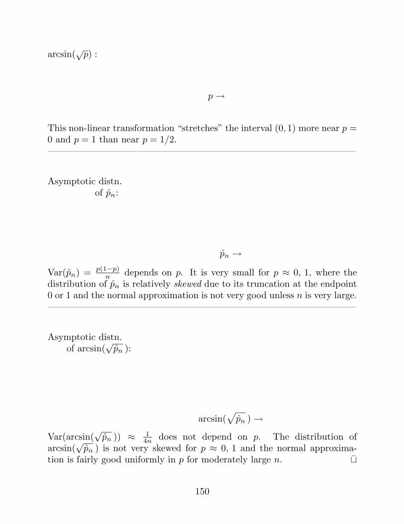
arcsin(√
p) :
p →
This non-linear transformation “stretches” the interval (0, 1) more near p =0 and p = 1 than near p = 1/2.————————————————————————————————–
Asymptotic distn.of pn:
pn →
Var(pn) = p(1−p)n depends on p. It is very small for p ≈ 0, 1, where the
distribution of pn is relatively skewed due to its truncation at the endpoint0 or 1 and the normal approximation is not very good unless n is very large.————————————————————————————————–
Asymptotic distn.of arcsin(
√pn ):
arcsin(√
pn ) →
Var(arcsin(√
pn )) ≈ 14n does not depend on p. The distribution of
arcsin(√
pn ) is not very skewed for p ≈ 0, 1 and the normal approxima-tion is fairly good uniformly in p for moderately large n.
150
Remark 10.6. A variance-stabilizing transformation can be used to makecomparisons between two or more parameters based on independent sam-ples. For example, if mp1 ∼ Binomial(m, p1) and np2 ∼ Binomial(n, p2)with m → ∞ and n → ∞ s.t. m
n → γ (0 < γ < ∞), then [verify]
√n
[(arcsin(
√p1 ) − arcsin(
√p2 )
)− (arcsin(
√p1 ) − arcsin(
√p2 ))
]d→ N1
(0,
14
+14γ
).(10.51)
Thus(arcsin(
√p1 ) − arcsin(
√p2 )
)±
√1+γ4nγ zα
2is an approximate (1 − α)-
confidence interval for (arcsin(√
p1 ) − arcsin(√
p2 )), which can in turn beused to test the hypothesis p1 = p2 vs. p1 = p2.
Exercise 10.6. (i) Assume Xλ ∼ Poisson(λ). Find a variance-stabilizingtransformation for Xλ as λ → ∞. That is, find a function h and constantc > 0 s.t.
(10.52) [h(Xλ) − h(λ)] d→ N1(0, c).
Use this to obtain an approximate (1 − α)-confidence interval for λ.Hint: Write λ = nθ with n → ∞ and θ the fixed unknown parameter.
(ii) Let Xλ ∼ Poisson(λ) and Xµ ∼ Poisson(µ), where Xλ ⊥⊥ Xµ and λand µ are both large. Based on (i), describe an approximate procedure fortesting λ = µ vs. λ = µ.
151
10.5. Asymptotic distribution of a sample covariance matrix.
Let W1 ≡(
X1
Y1
), . . . , Wn ≡
(Xn
Yn
)be an i.i.d. sample from a bivariate
distribution with finite fourth moments. Let
(10.53)
E(
Xi
Yi
)=
(µν
)≡ ξ,
Cov(
Xi
Yi
)=
(σ2 ρστρστ τ2
)≡
(σ 00 τ
) (1 ρρ 1
) (σ 00 τ
)≡ Σ.
The sample covariance matrix is defined to be
Sn =1
n − 1
∑n
i=1(Wi − Wn)(Wi − Wn)′(10.54)
=1
n − 1
∑(Xi − Xn)2
∑(Xi − Xn)(Yi − Yn)∑
(Xi − Xn)(Yi − Yn)∑
(Yi − Yn)2
.(10.55)
First, Sn is an unbiased, consistent estimator of Σ. To see this, set
Vi =(
Xi − µYi − ν
)≡ Wi − ξ,
so E(Vi) = 0, Cov(Vi) = Σ, Cov(Vn) = 1nΣ. Then from (10.54),
E(Sn) =1
n − 1E
[∑(Vi − Vn)(Vi − Vn)′
]=
1n − 1
E[∑
ViV′i − nVnV ′
n
](10.56)
=1
n − 1[n Cov(Vi) − n Cov(Vn)
]=
1n − 1
[n Σ − n · 1
nΣ
]= Σ ,
152
so Sn is unbiased. Also, Sn is consistent: from (10.56) and the WLLN,
(10.57) Sn =n
n − 1
(1n
∑ViV
′i − VnV ′
n
)p→ Σ.
We wish to determine the limiting distribution of√
n(Sn−Σ) as n → ∞(recall Example 10.4 re s2
n), from which we can determine, for example, thelimiting distribution of the sample correlation coefficient. Since Sn are 2×2symmetric matrices, equivalently we can consider the limiting distributionof the 3 × 1 rvtr
√n(Sn − Σ), where for any 2 × 2 symmetric matrix,
˜(a bb c
)=
abc
.
Note that this mapping A → A is a linear operation. Thus from (10.57),Sn and Σ are the 3-dimensional vectors
Sn =n
n − 1
(1n
∑ViV ′
i − ˜VnV ′n
)
≡ 1n − 1
∑(Xi − Xn)2∑
(Xi − Xn)(Yi − Yn)∑(Yi − Yn)2
,
Σ =
σ2
ρσττ2
.(10.58)
If we denote the 3-dimensional rvtr ViV ′i by
(10.59) Zi = ViV ′i =
(Xi − µ)2
(Xi − µ)(Yi − ν)(Yi − ν)2
,
then Z1, . . . , Zn are i.i.d., E(Zi) = Σ, and
Cov(Zi) =
κ40σ4 κ31σ
3τ κ22σ2τ2
κ31σ3τ κ22σ
2τ2 κ13στ3
κ22σ2τ2 κ13στ3 κ04τ
4
− Σ Σ′
≡ D(σ, τ)[K − R(ρ)R(ρ)′]D(σ, τ)(10.61)≡ Λ,
153
where (recall (10.25))
(10.62) κjk = E
[(Xi − µ
σ
)j (Yi − ν
τ
)k]
,
D(σ, τ) =
σ2 0 00 στ 00 0 τ2
, K =
κ40 κ31 κ22
κ31 κ22 κ13
κ22 κ13 κ04
, R(ρ) =
1ρ1
.
(The factorization (10.61) shows how the scale parameters σ and τ , thestandardized fourth moments κj,k, and the correlation ρ contribute to thecovariance matrix of Zi, hence to that of Sn.) Thus the CLT yields
(10.63)√
n(
Zn − Σ)
d→ N3(0, Λ).
so if we can show that
(10.64) ∆ ≡√
n(
Zn − Σ)−
√n
(Sn − Σ
)p→ 0,
then it will follow from (10.63) and Slutsky’s Theorem that
(10.65)√
n(Sn − Σ
)d→ N3(0, Λ).
By linearity, however,
∆ =√
n(
Zn − Sn
)=
√n ˜(
Zn − Sn
)and Zn = 1
n
∑ViV
′i , so from (10.57) we obtain (10.64):
√n
(Zn − Sn
)=
√n
[1n
∑ViV
′i − n
n − 1
(1n
∑ViV
′i − VnV ′
n
)]=
√n
n − 1
(nVnV ′
n − 1n
∑ViV
′i
)p→ 0 [verify].
154
Example 10.8 (Consistency and asymptotic distribution of the samplecorrelation coefficient and Fisher’s z-transform.) The sample correlation rn
is a consistent estimator of the population correlation ρ: since
(10.66) rn ≡1
n−1
∑(Xi − Xn)(Yi − Yn)√
1n−1
∑(Xi − Xn)2
√1
n−1
∑(Yi − Yn)2
= g(Sn),
where
(10.67) g(x, y, z) ≡ y√x√
z
is continuous for x, y > 0, and since Snp→ Σ by (10.57), we have that
(10.68) rnp→ ρ as n → ∞.
Exercise 10.7. (i) Apply (10.65) to find the asymptotic distribution of√n (rn−ρ). Express the asymptotic variance in terms of ρ and the moments
κjk in (10.62). (Since rn is invariant under location and scale changes, itsdistribution does not depend on µ, ν, σ, or τ .)
(ii) Specialize the result in (i) to the bivariate normal case, i.e., assume that(Xi
Yi
)∼ N2
[(µν
),
(σ2 ρστρστ τ2
)≡ Σ
][Evaluate the κjk in (10.62).]
(iii) In (ii), find a variance-stabilizing tranformation for rn. That is, finda function g(rn) such that
√n [g(rn) − g(ρ)] d→ N1(0, c) where c does not
depend on ρ (specify c).
155
10.6. Asymptotic distribution of sample quantiles.
Let X1, . . . , Xn be an i.i.d. sample from a continuous distribution on R1
with unknown cdf F . We shall show that for (0 < p < 1), the p-th samplequantile X([np]+1) ≡ F−1
n (p) is a CAN estimator of the p-th populationquantile ≡ F−1(p). That is, we shall show:
(10.69) X([np]+1)p→ F−1(p)
provided that F−1 exists and is continuous at p;
(10.70)√
n(X([np]+1) − F−1(p)
) d→ N1
(0,
p(1 − p)[f(F−1(p))]2
)provided that F−1 exists and is differentiable at p. (This requires thatf(F−1(p)) > 0.)
To derive (10.69) and (10.70), first consider the case where U1, . . . , Un
are i.i.d. Uniform(0,1) rvs with cdf G(u) = u, 0 ≤ u ≤ 1 (recall §10.1). From(10.4) and (10.5) we know that the empirical cdf Gn(u) ∼ 1
nBinomial(n, u)is a CAN estimator of G(u):
Gn(u)p→ G(u),(10.71)
√n [Gn(u) − G(u)] d→ N1 ( 0, u(1 − u) ) .(10.72)
Let 0 < U(1) < · · · < U(n) < 1 be the order statistics based on U1, . . . , Un.
Proposition 10.1. U([np]+1)p→ p (≡ G−1(p)).
Proof. Fix ε > 0. ThenU([np]+1) ≤ p − ε
= [np] + 1 or more U ′
is ≤ p − ε
=
Gn(p − ε) ≥ [np] + 1n
.
But Gn(p − ε)p→ p − ε and [np]+1
n → p (since |np − ([np] + 1)| ≤ 1), so
P[U([np]+1) ≤ p − ε
]→ 0 as n → ∞.
Similarly,
P[U([np]+1) ≥ p + ε
]→ 0 as n → ∞.
156
Proof of (10.69): Since (X1, . . . , Xn) distn= (F−1(U1), . . . , F−1(Un)),
(X(1), . . . , X(n))distn= (F−1(U(1)), . . . , F−1(U(n)) )(10.73)
because F is increasing, so
X([np]+1)distn= F−1(U([np]+1)).(10.74)
Since F−1 is assumed continuous at p, X([np]+1)p→ F−1(p) by Prop. 10.1.
Proposition 10.2.
(10.75)√
n(U([np]+1) − p
) d→ N1 ( 0, p(1 − p) ) .
Heuristic proof: By (10.71), Gn ≈ G. Thus√
n(U([np]+1) − p
)=
√n
[G−1
n (p) − p]
≈√
n[G−1
n (p) − G−1n (Gn(p))
]≈
√n[ p − Gn(p) ] [since G−1
n ≈ G−1 = ident.]d→ N1 ( 0, p(1 − p) ) [by (10.72)].
Rigorous proof: First, for any t ∈ R1,√n
(U([np]+1) − p
)≤ t
=
U([np]+1) ≤ p +
t√n
=
[np] + 1 or more U ′
is ≤ p +t√n
=
Gn
(p +
t√n
)≥ [np] + 1
n
= An + Bn + Cn ≥ −t
where ( (10.76) is verified below)
An ≡√
n
[Gn
(p +
t√n
)− Gn(p) − t√
n
]p→ 0,(10.76)
Bn ≡√
n [Gn(p) − p ] d→ N1 ( 0, p(1 − p) ) , [by (10.72)](10.77)
Cn ≡√
n
[p −
([np] + 1
n
)]=
|np − ([np] + 1)|√n
≤ 1√n→ 0.(10.78)
157
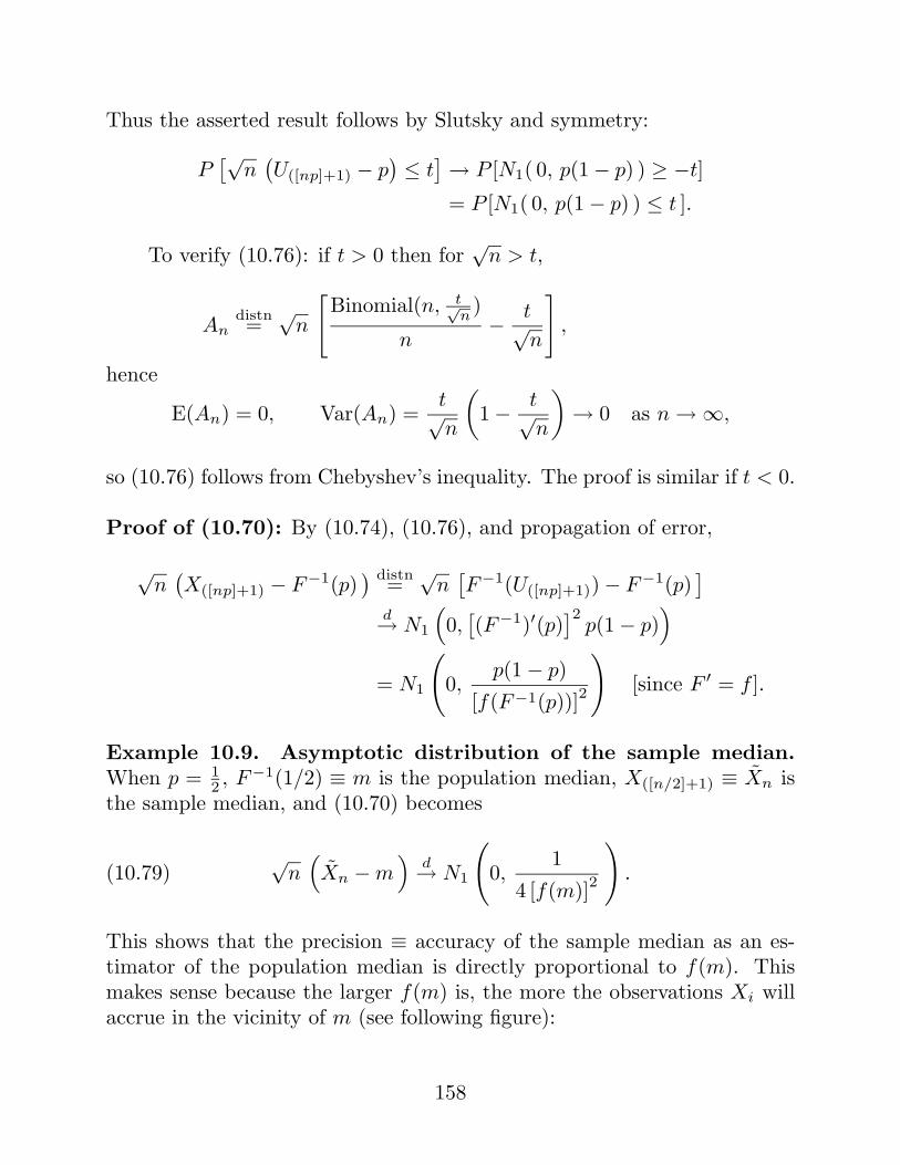
Thus the asserted result follows by Slutsky and symmetry:
P[√
n(U([np]+1) − p
)≤ t
]→ P [N1( 0, p(1 − p) ) ≥ −t]
= P [N1( 0, p(1 − p) ) ≤ t ].
To verify (10.76): if t > 0 then for√
n > t,
Andistn=
√n
[Binomial(n, t√
n)
n− t√
n
],
hence
E(An) = 0, Var(An) =t√n
(1 − t√
n
)→ 0 as n → ∞,
so (10.76) follows from Chebyshev’s inequality. The proof is similar if t < 0.
Proof of (10.70): By (10.74), (10.76), and propagation of error,
√n
(X([np]+1) − F−1(p)
) distn=√
n[F−1(U([np]+1)) − F−1(p)
]d→ N1
(0,
[(F−1)′(p)
]2p(1 − p)
)= N1
(0,
p(1 − p)[f(F−1(p))]2
)[since F ′ = f ].
Example 10.9. Asymptotic distribution of the sample median.When p = 1
2 , F−1(1/2) ≡ m is the population median, X([n/2]+1) ≡ Xn isthe sample median, and (10.70) becomes
(10.79)√
n(Xn − m
)d→ N1
(0,
14 [f(m)]2
).
This shows that the precision ≡ accuracy of the sample median as an es-timator of the population median is directly proportional to f(m). Thismakes sense because the larger f(m) is, the more the observations Xi willaccrue in the vicinity of m (see following figure):
158
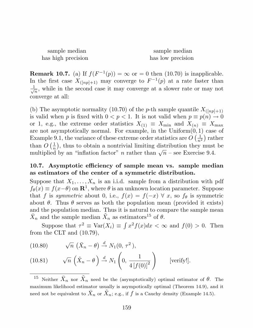
sample median sample medianhas high precision has low precision
Remark 10.7. (a) If f(F−1(p)) = ∞ or = 0 then (10.70) is inapplicable.In the first case X([np]+1) may converge to F−1(p) at a rate faster than1√n, while in the second case it may converge at a slower rate or may not
converge at all:
(b) The asymptotic normality (10.70) of the p-th sample quantile X([np]+1)
is valid when p is fixed with 0 < p < 1. It is not valid when p ≡ p(n) → 0or 1, e.g., the extreme order statistics X(1) ≡ Xmin and X(n) ≡ Xmax
are not asymptotically normal. For example, in the Uniform(0, 1) case ofExample 9.1, the variance of these extreme order statistics are O
(1
n2
)rather
than O(
1n
), thus to obtain a nontrivial limiting distribution they must be
multiplied by an “inflation factor” n rather than√
n – see Exercise 9.4.
10.7. Asymptotic efficiency of sample mean vs. sample medianas estimators of the center of a symmetric distribution.Suppose that X1, . . . , Xn is an i.i.d. sample from a distribution with pdffθ(x) ≡ f(x−θ) on R1, where θ is an unknown location parameter. Supposethat f is symmetric about 0, i.e., f(x) = f(−x) ∀ x, so fθ is symmetricabout θ. Thus θ serves as both the population mean (provided it exists)and the population median. Thus it is natural to compare the sample meanXn and the sample median Xn as estimators15 of θ.
Suppose that τ2 ≡ Var(Xi) ≡∫
x2f(x)dx < ∞ and f(0) > 0. Thenfrom the CLT and (10.79),
√n
(Xn − θ
) d→ N1(0, τ2 ),(10.80)
√n
(Xn − θ
)d→ N1
(0,
14 [f(0)]2
)[verify!].(10.81)
15 Neither Xn nor Xn need be the (asymptotically) optimal estimator of θ. The
maximum likelihood estimator usually is asympotically optimal (Theorem 14.9), and it
need not be equivalent to Xn or Xn; e.g., if f is a Cauchy density (Example 14.5).
159

Thus the asymptotic efficiency of Xn relative to Xn (as measured by theratio of their asymptotic variances) is 4[f(0)]2τ2.
Example 10.10. If Xi ∼ N1(θ, 1) (so τ2 = 1), then f(x) = 1√2π
e−x22 , so
(10.82) 4[f(0)]2τ2 =2π
≈ 0.637,
hence Xn is (asymptotically) less efficient than Xn: in the normal case theprecision of the sample median based on n observations is about the sameas that of the sample mean based on only .637n observations.
Actually, this should not be interpreted as a strong argument in favorof Xn. The efficiency of the sample median Xn relative to Xn is about64%, which, while a significant loss, is not catastrophic. If, however, ourassumption of a normal model is wrong, then the performance of the samplemean Xn may itself be catastrophic. For example, if f(x) ≡ 1
π(1+x2) is the
standard Cauchy density then the asymptotic variance of√
n(Xn − θ) is
(10.83)1
4[f(0)]2=
π2
4≈ 2.47,
but τ2 = ∞ so the asymptotic variance of Xn is infinite. In fact, Xn is noteven a consistent estimator of θ. Because of this, we say that the samplemedian is a robust estimator of the location parameter θ (for heavy-taileddepartures from normality), whereas the sample mean is not robust.Note: in the Cauchy case the sample median, while robust, is not optimal:the MLE is better (see Exercise 14.36(i)).
Exercise 10.8. Let f(x) ≡ 12e−|x| be the standard double exponential
density on R1, so fθ(x) = 12e−|x−θ|.
(i) Find the asymptotic efficiency of the sample median Xn relative to thesample mean Xn as estimators of θ.
(ii) Find the MLE θ for θ, i.e., the value of θ that maximizes the joint pdf
(10.84) fθ(x1, . . . , xn) ≡ 12n
n∏i=1
e−|xi−θ|.
160
Top Related