TTP12-048SFB/CPP-12-103

Penguin diagrams in the charm sector in K+ → π+νν

J. Mondejar and J. Rittinger

Institut fur Theoretische Teilchenphysik, Karlsruhe Institute of Technology (KIT),

Wolfgang-Gaede-Straße 1, 726128 Karlsruhe, Germany

Abstract

We evaluate at next-to-next-to-leading order (NNLO) the QCD corrections to thecharm contribution from penguin diagrams to the decay K+ → π+νν. A NNLOcalculation is already available in the literature [1]. We provide an independentcheck of the results of non-anomalous and anomalous diagrams. We use Renormal-ization Group improvement and an effective theory framework to resum the largelogarithms that appear. In the case of the non-anomalous diagrams, our results forthe decoupling coefficients and anomalous dimensions, as well as the final numericalresult, are in agreement with those of Ref. [1]. In the anomalous case, analyticaland numerical disagreements are observed.

1 Introduction

The rare decay mode K+ → π+νν, along with KL → π0νν, plays an important rolein flavor physics. It probes the quantum structure of flavor dynamics in the StandardModel (SM) [1–8] or its extensions [9–13] while remaining theoretically clean. A recentreview can be found in Ref. [14]. The cleanness of this decay is the main reason behindits importance, and it is due to the following:

• It being a semi-leptonic process, the relevant hadronic operator is just a currentoperator whose matrix element can be extracted from the leading decay K+ →π0e+ν, including isospin-breaking corrections [15].

• It is short-distance dominated. Long-distance contributions turn out to be small[16], and in principle calculable by means of lattice QCD [17].

1

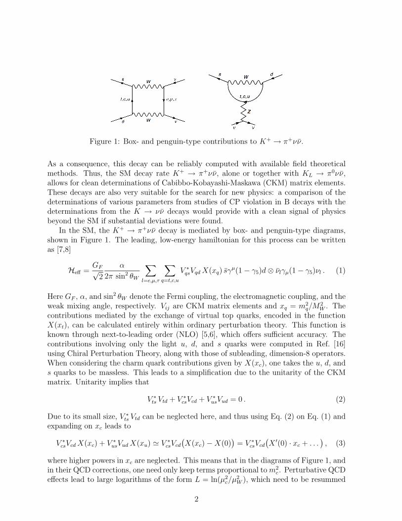
Figure 1: Box- and penguin-type contributions to K+ → π+νν.

As a consequence, this decay can be reliably computed with available field theoreticalmethods. Thus, the SM decay rate K+ → π+νν, alone or together with KL → π0νν,allows for clean determinations of Cabibbo-Kobayashi-Maskawa (CKM) matrix elements.These decays are also very suitable for the search for new physics: a comparison of thedeterminations of various parameters from studies of CP violation in B decays with thedeterminations from the K → νν decays would provide with a clean signal of physicsbeyond the SM if substantial deviations were found.

In the SM, the K+ → π+νν decay is mediated by box- and penguin-type diagrams,shown in Figure 1. The leading, low-energy hamiltonian for this process can be writtenas [7,8]

Heff =GF√

2

α

2π sin2 θW

∑l=e,µ,τ

∑q=t,c,u

V ∗qsVqdX(xq) sγ

µ(1− γ5)d⊗ νlγµ(1− γ5)νl . (1)

Here GF , α, and sin2 θW denote the Fermi coupling, the electromagnetic coupling, and theweak mixing angle, respectively. Vij are CKM matrix elements and xq = m2

q/M2W . The

contributions mediated by the exchange of virtual top quarks, encoded in the functionX(xt), can be calculated entirely within ordinary perturbation theory. This function isknown through next-to-leading order (NLO) [5,6], which offers sufficient accuracy. Thecontributions involving only the light u, d, and s quarks were computed in Ref. [16]using Chiral Perturbation Theory, along with those of subleading, dimension-8 operators.When considering the charm quark contributions given by X(xc), one takes the u, d, ands quarks to be massless. This leads to a simplification due to the unitarity of the CKMmatrix. Unitarity implies that

V ∗ts Vtd + V ∗

csVcd + V ∗usVud = 0 . (2)

Due to its small size, V ∗ts Vtd can be neglected here, and thus using Eq. (2) on Eq. (1) and

expanding on xc leads to

V ∗csVcdX(xc) + V ∗

usVudX(xu) ' V ∗csVcd

(X(xc)−X(0)

)= V ∗

csVcd(X ′(0) · xc + . . .

), (3)

where higher powers in xc are neglected. This means that in the diagrams of Figure 1, andin their QCD corrections, one need only keep terms proportional tom2

c . Perturbative QCDeffects lead to large logarithms of the form L = ln(µ2

c/µ2W ), which need to be resummed

2

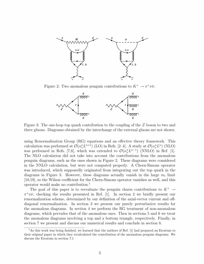
Figure 2: Two anomalous penguin contributions to K+ → π+νν.

Figure 3: The one-loop top quark contribution to the coupling of the Z boson to two andthree gluons. Diagrams obtained by the interchange of the external gluons are not shown.

using Renormalization Group (RG) equations and an effective theory framework. Thiscalculation was performed at O(αnsL

n+1) (LO) in Refs. [2–4]. A study at O(αnsLn) (NLO)

was performed in Refs. [7,8], which was extended to O(αnsLn−1) (NNLO) in Ref. [1].

The NLO calculation did not take into account the contributions from the anomalouspenguin diagrams, such as the ones shown in Figure 2. These diagrams were consideredin the NNLO calculation, but were not computed properly. A Chern-Simons operatorwas introduced, which supposedly originated from integrating out the top quark in thediagrams in Figure 3. However, these diagrams actually vanish in the large mt limit[18,19], so the Wilson coefficient for the Chern-Simons operator vanishes as well, and thisoperator would make no contribution.1

The goal of this paper is to reevaluate the penguin charm contributions to K+ →π+νν, checking the results presented in Ref. [1]. In section 2 we briefly present ourrenormalization scheme, determined by our definition of the axial-vector current and off-diagonal renormalization. In section 3 we present our purely perturbative results forthe anomalous diagrams. In section 4 we perform the RG treatment of non-anomalousdiagrams, which pervades that of the anomalous ones. Then in sections 5 and 6 we treatthe anomalous diagrams involving a top and a bottom triangle, respectively. Finally, insection 7 we present and discuss our numerical results and conclude in section 8.

1As this work was being finished, we learned that the authors of Ref. [1] had prepared an Erratum totheir original paper in which they recalculated the contribution of the anomalous penguin diagrams. Wediscuss the Erratum in section 7.1

3

2 Definition of the axial-vector current and off-diagonal

renormalization

We perform our calculations using dimensional regularization and the MS renormalizatonscheme. Beyond this, our scheme is determined by our choice of renormalization for theaxial-vector current and off-diagonal corrections to the quark propagator.

2.1 The axial-vector current

In dimensional regularization special attention must be paid to the definition of γ5. When-ever it appears in an open fermion line we can safely use its naive definition, but in closedloops we use the original definition by ’t Hooft and Veltman [20],

γ5 = i1

4!εν1ν2ν3ν4γν1γν2γν3γν4 . (4)

The Levi-Civita ε tensor is unavoidably a four-dimensional object and thus is taken out-side the R-operation where a D-dimensional object can be safely considered as a four-dimensional one. The gamma matrices are taken as D-dimensional inside the R-operation.With this definition γ5 no longer anticommutes with D-dimensional γµ. For this reasonwe use the definition of the axial-vector current presented in Ref. [21],

Aq,0 =1

2ψq (γµγ5 − γ5γµ)ψq → i

1

3!εµν1ν2ν3ψqγν1γν2γν3ψq . (5)

The renormalized current is defined as AqR = ξNSI

(ZNSAq0 + Zψ AS

0

), where AS =

∑q A

q

[21]. The renormalization constant ZNS cancels divergences arising from non-anomalousdiagrams, whereas Zψ deals with anomalous ones, and thus begins at order α2

s. Thecoefficient ξNS

I is a finite piece that is determined by requiring that the matrix elementsof the renormalized non-singlet axial-vector and vector vertices coincide,

ξNSI 〈ψγµγ5T

aψ〉R = 〈ψγµT aψ〉Rγ5 , (6)

where T a is the generator of a flavor group. This effectively restores the anticommutativityof the γ5 matrix for the non-singlet vertex, and so the standard Ward identities as well.This also means that the non-singlet axial-vector current defined in this way has zeroanomalous dimension.

2.2 Off-diagonal renormalization

The W and φ bosons can lead to flavor-changing corrections to the quark propagator,which in turn imply the appearance of reducible contributions to the penguin-type di-agrams, such as the one in Figure 4. In order to avoid these diagrams, we choose torenormalize the left-handed doublets in the following way [22–24],(

ud′

)0

L

= Z1/21

(ud′

)RL

,

(cs′

)0

L

= Z1/22

(cs′

)RL

, (7)

4

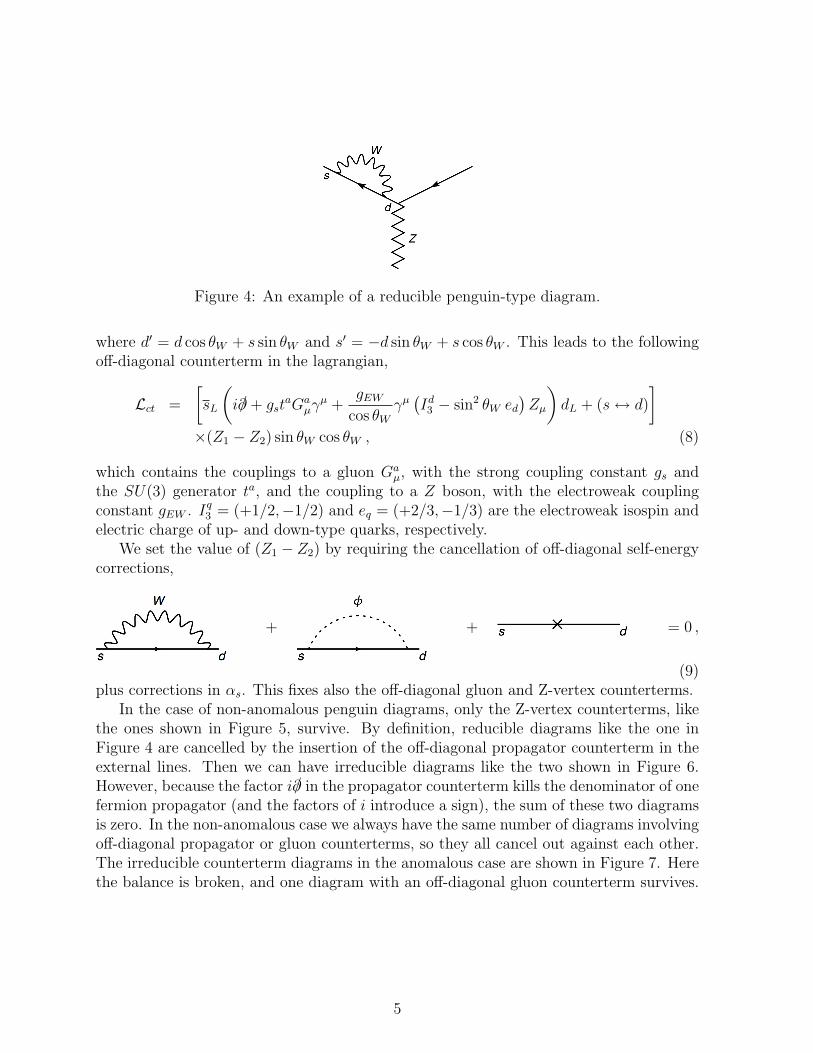
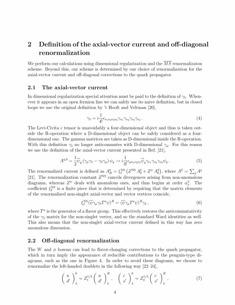
Figure 4: An example of a reducible penguin-type diagram.

where d′ = d cos θW + s sin θW and s′ = −d sin θW + s cos θW . This leads to the followingoff-diagonal counterterm in the lagrangian,

Lct =

[sL

(i/∂ + gst

aGaµγ

µ +gEW

cos θWγµ(Id3 − sin2 θW ed

)Zµ

)dL + (s↔ d)

]×(Z1 − Z2) sin θW cos θW , (8)

which contains the couplings to a gluon Gaµ, with the strong coupling constant gs and

the SU(3) generator ta, and the coupling to a Z boson, with the electroweak couplingconstant gEW . Iq3 = (+1/2,−1/2) and eq = (+2/3,−1/3) are the electroweak isospin andelectric charge of up- and down-type quarks, respectively.

We set the value of (Z1 − Z2) by requiring the cancellation of off-diagonal self-energycorrections,

+ + = 0 ,

(9)plus corrections in αs. This fixes also the off-diagonal gluon and Z-vertex counterterms.

In the case of non-anomalous penguin diagrams, only the Z-vertex counterterms, likethe ones shown in Figure 5, survive. By definition, reducible diagrams like the one inFigure 4 are cancelled by the insertion of the off-diagonal propagator counterterm in theexternal lines. Then we can have irreducible diagrams like the two shown in Figure 6.However, because the factor i/∂ in the propagator counterterm kills the denominator of onefermion propagator (and the factors of i introduce a sign), the sum of these two diagramsis zero. In the non-anomalous case we always have the same number of diagrams involvingoff-diagonal propagator or gluon counterterms, so they all cancel out against each other.The irreducible counterterm diagrams in the anomalous case are shown in Figure 7. Herethe balance is broken, and one diagram with an off-diagonal gluon counterterm survives.

5

Figure 5: Off-diagonal Z-vertex counterterms at zero and one loops.

Figure 6: Two irreducible diagrams involving off-diagonal counterterms.

Figure 7: The counterterm diagrams for the anomalous case.

3 Perturbative results for anomalous diagrams

Since the anomalous diagrams where initially computed incorrectly in Ref. [1], we willshow their calculation in detail, and begin by the perturbative results from their dia-grammatic calculations. We used the program qgraf [25] to generate all of the diagrams,and the packages q2e and exp [26,27] to express them as a series of vertices and propa-gators that can be read and evaluated by the FORM [28] package MATAD 3 [29].

For greater convenience when resumming logarithms later on, we will express theresults in terms of the operator Qν(µ), defined as

Qν(µ) =m2c(µ)

g2s(µ)µ2ε

sγµ(1− γ5)d , (10)

6

and write the expression for the charm contribution to Heff as

Hceff =

GF√2

α

2π sin2 θW

π2

2M2W

V ∗csVcdHν ⊗

∑l=e,µ,τ

νlγµ(1− γ5)νl

=g4EW

128M4W

V ∗csVcdHν ⊗

∑l=e,µ,τ

νlγµ(1− γ5)νl , (11)

where we have defined Hν = DQν(µ) and split up the global factor comming from theexternal neutrinos. We factored out the factor π2/(2M2

W ) so that the coefficient D willhave the same normalization as the decoupling coefficients in Refs. [1,7]. The relationbetween X, defined in Eq. (1), and D is simply X = π2/(2M2

W )m2c/g

2s D.

Because of the different logarithms that appear in them, we divide the coefficient Din different contributions, D = DW,t +DW,b +Dφ. Here DW,t stands for diagrams with aW boson and a top triangle, DW,b for diagrams with W and a bottom triangle, and Dφ

contains all anomalous diagrams with Goldstone bosons ( `µ/mX= ln[µ2/m2

X(µ)] )

DW,t =(a(6)(µ)

)3

12CF

[(1− 4`µ/mt

)(1 + `µ/MW

− `µ/mc

)], (12)

DW,b =(a(6)(µ)

)3

4CF

[6`2µ/MW

+ 6`2µ/mb− 12`µ/mb

`µ/mc + 9`µ/MW+ 3`µ/mc + 36 + 2π2

],

(13)

Dφ = −(a(6)(µ)

)3

CF

[6`2µ/mt

+ 6`2µ/MW− 12`µ/mt(3 + `µ/MW

) + 36`µ/MW+ 75 + 2π2

],

(14)

D =(a(6)(µ)

)3

3CF

[8`2MW /mb

− 2`2MW /mt− 16`MW /mb

`MW /mc − 4`MW /mt(1− 4`MW /mc)

+ 2π2 + 27], (15)

with a(nf) = α(nf )s /(4π) being the QCD coupling constant in the effective nf flavor theory

and CF = 4/3. One can see by inspecting Eqs. (12)-(14) that the explicit `µ dependencecancels separately in Dφ and the sum DW,t +DW,b.

As they are, the results from the diagrams involving the W boson are of little usebecause of the large logarithms present in them, and an RG treatment is called for.However, as we can see in (14) the Goldstone contribution only contains the W and topquark scale, which are of similar size. We won’t treat this contribution when we proceedwith the RG improvement in the effective field theory language.

4 RG improvement: non-anomalous diagrams

Part of the goal of this paper is to check the results for non-anomalous penguin diagramsfrom Ref. [1]. These diagrams are always present as subgraphs in the anomalous case. Inparticular, we will need the Wilson coefficients and anomalous dimensions related to the

7

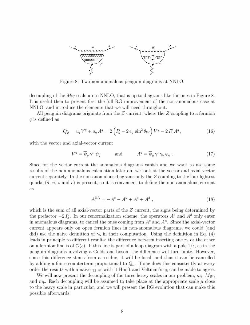
Figure 8: Two non-anomalous penguin diagrams at NNLO.

decoupling of the MW scale up to NNLO, that is up to diagrams like the ones in Figure 8.It is useful then to present first the full RG improvement of the non-anomalous case atNNLO, and introduce the elements that we will need throughout.

All penguin diagrams originate from the Z current, where the Z coupling to a fermionq is defined as

QqZ = vq V

q + aq Aq = 2

(Iq3 − 2 eq sin2 θW

)V q − 2 Iq3 A

q , (16)

with the vector and axial-vector current

V q = ψq γµ ψq and Aq = ψq γ

µγ5 ψq . (17)

Since for the vector current the anomalous diagrams vanish and we want to use someresults of the non-anomalous calculation later on, we look at the vector and axial-vectorcurrent separately. In the non-anomalous diagrams only the Z coupling to the four lightestquarks (d, u, s and c) is present, so it is convenient to define the non-anomalous currentas

ANA = −Ac − Au + As + Ad , (18)

which is the sum of all axial-vector parts of the Z current, the signs being determined bythe prefactor −2 Iq3 . In our renormalization scheme, the operators As and Ad only enterin anomalous diagrams, to cancel the ones coming from Ac and Au. Since the axial-vectorcurrent appears only on open fermion lines in non-anomalous diagrams, we could (anddid) use the naive definition of γ5 in their computation. Using the definition in Eq. (4)leads in principle to different results: the difference between inserting one γ5 or the otheron a fermion line is of O(ε). If this line is part of a loop diagram with a pole 1/ε, as in thepenguin diagrams involving a Goldstone boson, the difference will turn finite. However,since this difference stems from a residue, it will be local, and thus it can be cancelledby adding a finite counterterm proportional to Qν . If one does this consistently at everyorder the results with a naive γ5 or with ’t Hooft and Veltman’s γ5 can be made to agree.

We will now present the decoupling of the three heavy scales in our problem, mt, MW ,and mb. Each decoupling will be assumed to take place at the appropriate scale µ closeto the heavy scale in particular, and we will present the RG evolution that can make thispossible afterwards.

8

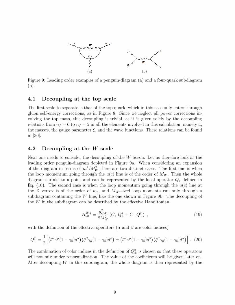
(a) (b)

Figure 9: Leading order examples of a penguin-diagram (a) and a four-quark subdiagram(b).

4.1 Decoupling at the top scale

The first scale to separate is that of the top quark, which in this case only enters throughgluon self-energy corrections, as in Figure 8. Since we neglect all power corrections in-volving the top mass, this decoupling is trivial, as it is given solely by the decouplingrelations from nf = 6 to nf = 5 in all the elements involved in this calculation, namely a,the masses, the gauge parameter ξ, and the wave functions. These relations can be foundin [30].

4.2 Decoupling at the W scale

Next one needs to consider the decoupling of the W boson. Let us therefore look at theleading order penguin-diagram depicted in Figure 9a. When considering an expansionof the diagram in terms of m2

c/M2W there are two distinct cases. The first one is when

the loop momentum going through the u(c) line is of the order of MW . Then the wholediagram shrinks to a point and can be represented by the local operator Qν defined inEq. (10). The second case is when the loop momentum going through the u(c) line atthe Z vertex is of the order of mc, and MW -sized loop momenta run only through asubdiagram containing the W line, like the one shown in Figure 9b. The decoupling ofthe W in the subdiagram can be described by the effective Hamiltonian

HW,qeff =

g2EW

8M2W

(C+Qq+ + C−Q

q−) , (19)

with the definition of the effective operators (α and β are color indices)

Qq± =

1

2

[(sαγµ(1− γ5)q

α)(qβγµ(1− γ5)d

β)±(sαγµ(1− γ5)q

β)(qβγµ(1− γ5)d

α)]. (20)

The combination of color indices in the definition of Qq± is chosen so that these operators

will not mix under renormalization. The value of the coefficients will be given later on.After decoupling W in this subdiagram, the whole diagram is then represented by the

9

bilocal operators

V± = −i∫

d4x T{ ∑q=d,u,s,c

(Qc±(x)−Qu

±(x))vq V

q(0)}, (21)

ANA± = −i

∫d4x T

{(Qc±(x)−Qu

±(x))ANA(0)

}, (22)

for the vector and axial-vector current, respectively. The minus sign between Qc± and Qu

±comes from the GIM mechanism discussed in Eq. (3).

Besides the operators Qq± one must also consider a set of evanescent operators Qq

Ei

(and the corresponding bilocal operators). We take the definitions from Ref. [1] (modifiedby a normalization factor), which we present in Appendix A. Evanescent operators vanishat four dimensions, but yield non-zero contributions when inserted in loop diagrams withpoles in ε. We choose a renormalization scheme for them in which their matrix elementsvanish and they do not mix with physical operators [31]. The physical operators still mixwith them, though, so the evanescents contribute to the anomalous dimensions of Qq

±,and, inserted into bilocal operators, to those of V± and ANA

± .Putting everything together, we describe the non-anomalous penguin-diagrams with

a vector and axial-vector current with the Hamiltonian

HNAν,eff = C+

[V+ + ANA

+

]+ C−

[V− + ANA

−]+ CNA

ν Qν , (23)

Here we have omitted the normalization and neutrino factors, which are the same as theones multiplying Hν in Eq. (11). The coefficients in HNA

ν,eff are ( `µW /MW= ln[µ2

W/M2W ] )

C+(µW ) = 1 + a(5)(µW )[

113

+ 2 `µW /MW

]+(a(5)(µW )

)2[`2µW /MW

(13− 2

3nf)

+ 518`µW /MW

(159− 8nf )

− 118

(55 + 24 ζ2)nf + 26 ζ2 + 217091800

], (24)

C−(µW ) = 1− a(5)(µW )[

223

+ 4 `µW /MW

]+(a(5)(µW )

)2[`2µW /MW

(− 14 + 4

3nf)− 5

9`µW /MW

(105− 8nf )

+ 19(55 + 24 ζ2)nf − 28 ζ2 − 92443

900

], (25)

CNAν (µW ) = a(5)(µW ) 8

[`µW /MW

+ 2]

+(a(5)(µW )

)2163

[12 `2µW /MW

+ 34 `µW /MW+ 24 ζ2 + 33

]+(a(5)(µW )

)3 [− 64

3`3µW /MW

(−24 + nf ) + `2µW /MW

(3408− 1024

9nf)

− 169`µW /MW

(− 5270− 1728 ζ2 + nf (161 + 72 ζ2) + 468 ζ3

)− 416 ζ4 − 8896

3ζ3 + 6816 ζ2 − 64

9nf (49 + 32 ζ2 − 12 ζ3)

+ 7995148675

]. (26)

10

The bilocal operators V± do not mix under the RG evolution with other operators andtheir matrix elements vanish. Therefore, we don’t have to consider the vector current anylonger, its only effect being inside the decoupling constant CNA

ν .

4.3 Decoupling at the bottom scale

First note that when decoupling a heavy quark, the non-singlet vector or axial-vectorcurrent is the same in the full and effective theory due to Ward identities [18,19,32]. Asa consequence, the non-anomalous current is the same in the five and four flavor theory([ANA](5) = [ANA](4)). Also, the decoupling coefficient for the Qν operator stems purelyfrom the prefactor m2

c/g2s , [

Qν

](5)= Bν

[Qν

](4), (27)

with ( `µb/mb= ln[µ2

b/m2b(µb)] )

Bν(µb) =1− 2

3a(5)(µb) `µb/mb

− 2

27

(a(5)(µb)

)2[30 `2µb/mb

+ 39 `µb/mb+ 56

]. (28)

The decoupling equations for the local operators Qq± are[

Qq±

](5)= B±

[Qq±

](4), (29)

with

B+(µb) =1− 1

54

(a(5)(µb)

)2[36 `2µb/mb

+ 12 `µb/mb+ 59

], (30)

B−(µb) =1 +1

27

(a(5)(µb)

)2[36 `2µb/mb

+ 12 `µb/mb+ 59

]. (31)

These results then can be used to get the decoupling coefficients for the bilocal operators,whose decoupling equations read[

ANA±

](5)

= B±

[ANA±

](4)+BNA

±,ν

[Qν

](4), (32)

with

BNA+,ν(µb) =

8

9

(a(5)(µb)

)3[12 `3µb/mb

− 96 `2µb/mb+ 261 `µb/mb

+ 96 ζ3 − 12793

], (33)

BNA−,ν,u(µb) =− 8

9

(a(5)(µb)

)3[12 `3µb/mb

− 96 `2µb/mb+ 241 `µb/mb

+ 96 ζ3 − 12313

]. (34)

11

4.4 Decoupling at the charm scale

At the charm scale one matches finally the operator ANA± to Qν and finds the coefficient

X(xc), cf. Eq. (1). The operator multiplying X has no anomalous dimension, whichmeans that X is independent of µ. In this case it is unnecessary to move to a three-flavortheory, and one stays in the four-flavor one,[

ANA±

](4)= CNA

±,ν

[Qν

](4), (35)

with the coefficients ( `µc/mc = ln[µ2c/m

2c(µc)] )

CNA+,ν(µc) =16 a(4)(µc)

[1− `µc/mc

]−(a(4)(µc)

)2[48`2µc/mc

− 80`µc/mc − 44], (36)

CNA−,ν(µc) =− 8 a(4)(µc)

[1− `µc/mc

]+

4

3

(a(4)(µc)

)2[36`2µc/mc

+ 36`µc/mc − 21]. (37)

After showing the decouplings at different scales, we now show how the operators can beevolved between these scales.

4.5 Running to different scales

The evolution of the operator Qν is given by

µ2 d

dµ2Qν(µ) = γν Qν(µ) , (38)

where γν is easily determined from the renormalization constants of mc and αs. Definingdµ2/µ2a = aβ(a),

γν = 2(γm − β) = a[3− 2

3nf

]− 2

9a2[147 + 37nf

]+

1

162a3[− 173259− 18705nf + 1535n2

f + 17280 ζ3nf

]. (39)

The solution of Eq. (38) is

Qν(µ) = Uν(µ, µ0)Qν(µ0) = exp

(∫ a(µ)

a(µ0)

dz

z

γν(z)

β(z)

)Qν(µ0) . (40)

Considering the RG equations for the local operators Q± and ANA

µ2 d

dµ2Qq±(µ) = γ±Q

q±(µ) , (41)

µ2 d

dµ2ANA(µ) = 0 , (42)

12

one gets for the bilocal operators

µ2 d

dµ2ANA± (µ) = γ±A

NA± (µ) + γNA

±,ν Qν(µ) . (43)

The anomalous dimensions are

γ+ = − 2 a+ a2[

72− 2

9nf

]+ a3

[− 275267

300+ 52891

1350nf + 130

81n2f +

(336 + 80

3nf)ζ3

], (44)

γ− = 4 a+ a2[7 + 4

9nf

]+ a3

[− 12297

50+ 31343

675nf − 260

81n2f −

(336 + 160

3nf)ζ3

], (45)

and

γNA+,ν = − 16 a− 144 a2 + a3

[− 1060082

225+ 144nf + 896 ζ3

], (46)

γNA−,ν = 8 a+ 208 a2 + a3

[879586

225− 144nf − 64 ζ3

]. (47)

The factor 1/g2s was introduced in the definition of Qν , cf. Eq. (10), so that the anomalous

dimensions γNA±,ν would begin at order a, and not a0. The solution of Eq. (43) is

ANA± (µ) = U±(µ, µ0)A

NA± (µ0) + UNA

±,ν(µ, µ0)Qν(µ0) , (48)

where

U±(µ, µ0) = exp

(∫ a(µ)

a(µ0)

dz

z

γ±(z)

β(z)

), (49)

UNA±,ν(µ, µ0) = exp

(∫ a(µ)

a(µ0)

dz

z

γ±(z)

β(z)

)·∫ a(µ)

a(µ0)

dz

z

γNA±,ν(z)

β(z)

· exp

(∫ z

a(µ0)

dz′

z′γν(z

′)− γ±(z′)

β(z′)

). (50)

4.6 Result

Using all the decoupling coefficients and evolution equations presented in the previoussections one can find the final result for the non-anomalous diagrams. We start by Eq. (23)with nf = 5, and evolve the operators down to a scale µb ∼ mb using Eqs. (40), (49) and(50). We decouple the b quark using Eqs. (27) and (32) and continue evolving the operatorswith nf = 4 down to a scale µc ∼ mc, where we express everything in terms of Qν usingEq. (35), and then find the expression of XNA. We define the masses mq ≡ mq(mq) andthe logs `µq/emq ≡ ln(µq/mq). Further, we define the factors

Kc =

(a(4)(µc)

a(4)(mc)

), L =

(a(4)(µc)

a(4)(µb)

) 125

, M =

(a(5)(µb)

a(5)(µW )

) 123

. (51)

13

Kc comes from expressing mc(µ) in terms of mc, and M and L from the evolution fromµW to µb and from µb to µc, respectively. With these conventions, our result reads

XNA =m2c

M2W

1

32 a(4)(µc)K

2425c

{487L−6M−6 + 24

11L12M12

+ L(− 744

65M−1 + 96

35M−6 − 48

143M12

)+ a(5)(µW )

[517843703

L−6M−6 − 749685819

L12M12 + L(

2888594103155

M−1 + 10356818515

M−6 + 14993675647

M12)

+ `µW /MW

(967L−6M−6 − 96

11L12M12 + L

(− 248

65M−1 + 192

35M−6 + 192

143M12

))]+ a(5)(µb)

[− 2609808

2314375L−6M−6 + 3769008

3636875L12M12 + L

(31752729621490625

M−1 − 59868879234715625

M−6

− 212453104141838125

M12 + `µb/emb

(49665M−1 − 32

5M−6 − 16

13M12

))]+ a(4)(µc)

[− 966244

13125L−6M−6 − 57302

6875L12M12 + `µc/emc

(− 16L−6M−6 + 8L12M12

)+ L

(377257640625

M−1 − 48678421875

M−6 + 24339289375

M12)]

+O(a2)

}. (52)

The O(a2) coefficient is simply too long to print here. The full result can be retrieved fromhttp://www-ttp.particle.uni-karlsruhe.de/Progdata/ttp12/ttp12-048/. We willgive numerical results for XNA in section 7. The expression above agrees with the result ofthe NLO calculation performed in Refs. [7,8], correcting for the fact that in those publica-tions no decoupling was performed at µb, and more importantly, that ln [µc/mc(µc)] wassimply changed by hand to ln [µc/mc(mc)], and so they are missing a couple terms relatedto Kc. Unfortunately, we could not readily compare the final expression of our full resultto that of Ref. [1], but we found agreement in the decoupling coefficients and anomalousdimensions leading to it (accounting in some cases for differences in normalization).

If we re-expand Eq. (52) around µW we obtain

XNA =m2c

M2W

{14

(`emc/MW

+ 3)

+ 2 a(5)(µW )[`2µW /µb

+ `2µW /MW+ `µb/µc

(16− `emc/MW

)+ `µb/emc

(`µc/emc − `µW /MW

− 4)

+ `µW /µb

(`µb/emc + `µc/emc − 2`µW /MW

− 236

)− `µW /MW

(`µc/emc − 23

6

)+ 1

6

(`µc/emc + 2π2 + 29

) ]+(a(5)(µW )

)2[83`3µW /µb

+ 3 `3µb/µc+ 1

3`2µb/emc

(`µc/emc − `µW /MW

+ 20)

+ 9 `2µb/µc

(`µW /µb

− `µW /MW+ `µc/emc + 5

18

)+ . . .

]+O

(a2`0

)}, (53)

where for brevity’s sake we only show a few terms of the long, last-order coefficient. If onedifferentiates this re-expanded expression with respect to the various µx scales present in

14

(a) (b) (c)

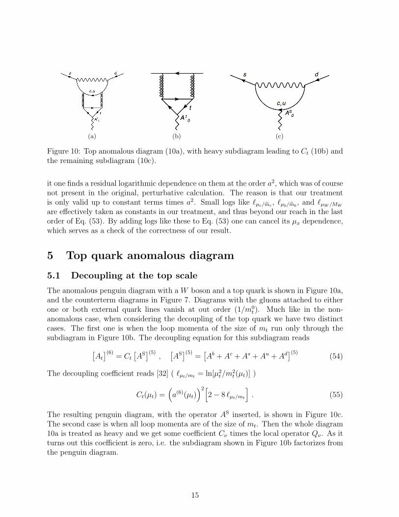
Figure 10: Top anomalous diagram (10a), with heavy subdiagram leading to Ct (10b) andthe remaining subdiagram (10c).

it one finds a residual logarithmic dependence on them at the order a2, which was of coursenot present in the original, perturbative calculation. The reason is that our treatmentis only valid up to constant terms times a2. Small logs like `µc/emc , `µb/emb

, and `µW /MW

are effectively taken as constants in our treatment, and thus beyond our reach in the lastorder of Eq. (53). By adding logs like these to Eq. (53) one can cancel its µx dependence,which serves as a check of the correctness of our result.

5 Top quark anomalous diagram

5.1 Decoupling at the top scale

The anomalous penguin diagram with a W boson and a top quark is shown in Figure 10a,and the counterterm diagrams in Figure 7. Diagrams with the gluons attached to eitherone or both external quark lines vanish at out order (1/m0

t ). Much like in the non-anomalous case, when considering the decoupling of the top quark we have two distinctcases. The first one is when the loop momenta of the size of mt run only through thesubdiagram in Figure 10b. The decoupling equation for this subdiagram reads[

At](6)

= Ct[AS](5)

,[AS](5)

=[Ab + Ac + As + Au + Ad

](5)(54)

The decoupling coefficient reads [32] ( `µt/mt = ln[µ2t/m

2t (µt)] )

Ct(µt) =(a(6)(µt)

)2[2− 8 `µt/mt

]. (55)

The resulting penguin diagram, with the operator AS inserted, is shown in Figure 10c.The second case is when all loop momenta are of the size of mt. Then the whole diagram10a is treated as heavy and we get some coefficient Cν times the local operator Qν . As itturns out this coefficient is zero, i.e. the subdiagram shown in Figure 10b factorizes fromthe penguin diagram.

15

5.2 Decoupling at the W scale

When decoupling the W we only have to treat the singlet penguin diagram in Figure 10c,which leads then, analogously to the non-anomalous problem, to the effective Lagrangian

Htν,eff = Ct

(C+A

S+ + C−A

S− + CS

ν Qν

), (56)

with the operator

AS± = −i

∫d4x T

{(Qc±(x)−Qu

±(x))AS(0)

}(57)

and the coefficient ( `µW /MW= ln[µ2

W/M2W ] )

CSν (µW ) = − a(5)(µW ) 8 (3 + `µW /MW

) . (58)

5.3 Decoupling at the bottom and charm scales

Because of the overall multiplying factor Ct, when decoupling the bottom quark we canneglect all terms of higher order than a2. This makes the decoupling equation quite trivial,[

AS±

](5)=[AS±

](4)+O

(a2). (59)

In the next section, when we treat the bottom anomalous diagrams, we will give thisdecoupling equation to a higher order. The singlet current in the five flavor theory containsthe bottom quark, while in the four flavor theory only the four lightest quarks are present.The decoupling equation for Qν is given in Eq. (27).

At the charm scale, the matching equation reads[AS±

](4)= CS

±,ν

[Qν

](4). (60)

At our order, this matching is influenced only by non-anomalous diagrams generatedby the Ac and Au currents. We got rid of non-anomalous contributions from As and Ad

with our off-diagonal renormalization scheme, so these operators could only enter throughanomalous diagrams. At the charm scale, however, these diagrams would only produceterms beyond our precision. Nevertheless, the matching for AS

± at this scale will not thesame as the one for ANA

± . Since ANA only appeared in open fermion lines we used thenaive definition of γ5 for it, but AS appears here through the decoupling of the current At,which is inserted in a closed triangle loop. We used the definition in Eq. (5) for At, anduse it too for AS. As mentioned in section 4, the different definitions of the axial-vectorcurrent produce different results for the penguin diagrams, which in turn leads to differentconstant parts in CS

±,ν compared to the coefficients CNA±,ν given in Eqs. (36) and (37),

( `µc/mc = ln[µ2c/m

2c(µc)] )

CS+,ν(µc) =16 a(4)(µc)

[2 + `µc/mc

]+(a(4)(µc)

)2[48`2µc/mc

− 80`µc/mc − 5243

], (61)

CS−,ν(µc) =− 8 a(4)(µc)

[2 + `µc/mc

]− 4

3

(a(4)(µc)

)2[36`2µc/mc

+ 36`µc/mc + 17]. (62)

16

The minus sign between these and the previous expressions comes from the different signswith which the currents Ac/u enter in the definitions of AS and ANA.

5.4 Running to different scales

In contrast to ANA the singlet operator AS has a non-vanishing anomalous dimension

µ2 d

dµ2AS(µ) = γSAS(µ) , (63)

with [19,21]

γS = −8nf a2 + a3

[− 340

3nf −

8

9n2f

]. (64)

The solution of Eq. (63) is

AS(µ) = US(µ, µ0)AS(µ0) = exp

(∫ a(µ)

a(µ0)

dz

z

γS(z)

β(z)

)AS(µ0) . (65)

For the bilocal operator we get the following RG equation,

µ2 d

dµ2AS±(µ) = γS

±AS±(µ) + γS

±,ν Qν(µ) , (66)

with γS± = γ± + γS and

γS+,ν = 16 a− 144 a2 + a3

[− 896 ζ3 + 800

9nf + 67682

225

], (67)

γS−,ν = −8 a+ 80 a2 + a3

[64 ζ3 + 560

9nf + 147614

225

]. (68)

The solution of Eq. (66) is

AS±(µ) = US

±(µ, µ0)AS±(µ0) + US

±,ν(µ, µ0)Qν(µ0) , (69)

with US± and US

±,ν defined as in Eqs. (49) and (50) with γ± (γNA±,ν) replaced by γS

± (γS±,ν).

5.5 Result

With the same definitions as in Eq. (51), our result for the top anomalous diagrams reads

XW,t =m2c

M2W

1

32 a(4)(µc)K

2425c ·

(a(6)(µt)

)2[2− 8 `µt/mt

][48

7L−6M−6 +

24

11L12M12

+ L

(−744

65M−1 +

96

35M−6 − 48

143M12

)]. (70)

17

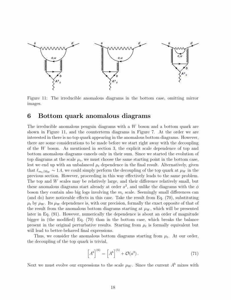
Figure 11: The irreducible anomalous diagrams in the bottom case, omitting mirrorimages.

6 Bottom quark anomalous diagrams

The irreducible anomalous penguin diagrams with a W boson and a bottom quark areshown in Figure 11, and the counterterm diagrams in Figure 7. At the order we areinterested in there is no top quark appearing in the anomalous bottom diagrams. However,there are some considerations to be made before we start right away with the decouplingof the W boson. As mentioned in section 3, the explicit scale dependence of top andbottom anomalous diagrams cancels only in their sum. Since we started the evolution oftop diagrams at the scale µt, we must choose the same starting point in the bottom case,lest we end up with an unbalanced µt dependence in the final result. Alternatively, giventhat `mt/MW

∼ 1.4, we could simply perform the decoupling of the top quark at µW in theprevious section. However, proceeding in this way effectively leads to the same problem.The top and W scales may be relatively large, and their difference relatively small, butthese anomalous diagrams start already at order a2, and unlike the diagrams with the φboson they contain also big logs involving the mc scale. Seemingly small differences can(and do) have noticeable effects in this case. Take the result from Eq. (70), substitutingµt by µW . Its µW dependence is, with our precision, formally the exact opposite of that ofthe result from the anomalous bottom diagrams starting at µW , which will be presentedlater in Eq. (91). However, numerically the dependence is about an order of magnitudebigger in (the modified) Eq. (70) than in the bottom case, which breaks the balancepresent in the original perturbative results. Starting from µt is formally equivalent butwill lead to better-behaved final expressions.

Thus, we consider the anomalous bottom diagrams starting from µt. At our order,the decoupling of the top quark is trivial,[

Ab](6)

=[Ab](5)

+O(a3) . (71)

Next we must evolve our expressions to the scale µW . Since the current Ab mixes with

18

AS under the RG evolution, we make use of the identity

Ab = Ab − 1

nfAS +

1

nfAS = ANS +

1

nfAS , (72)

with ANS = Ab − 1/nfAS, to express Ab through the non-mixing operators ANS and

AS. Our choice of renormalization scheme for the axial current, presented in section 2.1,ensures that ANS has a vanishing anomalous dimension. The evolution of AS was shownin Eq. (65). Thus, we have that[

Ab(µt)](5)

=[ANS(µW )

](5)

+1

5US(µt, µW )

[AS(µW )

](5)=[Ab(µW )

](5)

+(24

23

(a(5)(µt)− a(5)(µW )

)+O(a2)

)[AS(µW )

](5). (73)

The treatment of AS is now the same as in the top quark case, and exchanging Ct by thecoefficient from the expansion of US, the result will be the same as in Eq. (70), with asign coming from the different isospins of top and bottom quarks. This all leaves us with

the operator[Ab(µW )

](5)

, whose treatment we present in the following sections.

6.1 Decoupling at the W scale

As in the other cases we look at the different possible heavy subdiagrams to obtain theoperators and coefficients in the effective theory. The effective Hamiltonian reads

Hbν,eff = C+A

b+ + C−A

b− + Cb

ν Qν , (74)

with

Ab± = −i∫

d4x T{(Qc±(x)−Qu

±(x))Ab(0)

}, (75)

and ( `µW /MW= ln[µ2

W/M2W ] )

Cbν(µW ) =

(a(5)(µW )

)3 8

3

[55 + 4π2 + 18 `µW /MW

+ 12 `2µW /MW

]. (76)

We will apply the same replacement to the bilocal operator as in Eq. (72). The resultingoperators ANS

± and AS± can now be evolved separately from the W to the bottom scale.

6.2 Decoupling at the bottom and charm scales

For the local operators Qq± and Qν the decoupling equations are given in the previous

sections. For Ab the decoupling equation reads[Ab](5)

= Cb

[AS](4)

, (77)

19

with ( `µb/mb= ln[µ2

b/m2b(µb)] )

Cb(µb) =(a(5)(µb)

)2[2− 8 `µb/mb

](78)

in complete analogy to the top decoupling in (54). Unlike the top quark case, however, thecontribution from treating the whole diagram as heavy is not zero. Thus, the decouplingequation for the bilocal operator Ab± reads[

Ab±

](5)

= B±Cb

[AS±

](4)

+Bb±,ν

[Qν

](4). (79)

where the coefficients B± have been defined in Eq. (29), and Bb±,ν read

Bb+,ν(µb) = −

(a(5)(µb)

)3[64 `2µb/mb

+ 64 `µb/mb+ 368

3

], (80)

Bb−,ν(µb) =

(a(5)(µb)

)3[32 `2µb/mb

− 64 `µb/mb+ 328

3

]. (81)

At the order we are interested in, the operator Aq for the four lightest quarks decouplesnaively ([Aq](5) = [Aq](4) + O(a3)). Also, as in the previous section, As and Ad makeno contribution, since in our renormalization scheme they could only enter in anomalousdiagrams that would lie beyond our precision. The decoupling of the bottom quark in abilocal operator with an insertion of the current Ac + Au is given by[

A(c+u)±

](5)

= B±

[A

(c+u)±

](4)

+B(c+u)±,ν

[Qν

](4), (82)

with

B(c+u)+,ν (µb) =− 8

9

(a(5)(µb)

)3[12 `3µb/mb

+ 12 `2µb/mb+ 107 `µb/mb

+ 96 ζ3 − 361627

], (83)

B(c+u)−,ν,u (µb) =

8

9

(a(5)(µb)

)3[12 `3µb/mb

+ 12 `2µb/mb+ 95 `µb/mb

+ 96 ζ3 − 302027

]. (84)

At our order, the difference between B(c+u)±,ν and BNA

±,ν , besides an obvious sign, stems fromthe fact that here we are using the ’t Hooft-Veltman definition of γ5 instead of the naiveone that we used for the non-anomalous diagrams, as mentioned before. Using Eqs. (79)and (82), and remembering the definition ANS = Ab − 1/5AS we find at last that[

ANS±

](5)

= B±

(4

5Cb −

1

5

)[AS±

](4)+

(4

5Bb±,ν −

1

5B

(c+u)±,ν

)[Qν

](4)+O

(a3), (85)[

AS±

](5)

= B±

(Cb + 1

)[AS±

](4)

+(Bb±,ν + B

(c+u)±,ν

) [Qν

](4)

+O(a3). (86)

The matching at the charm scale is given in Eq. (60).

20

6.3 Running to different scales

The evolution of AS± was given in Eq. (69). ANS has a vanishing anomalous dimension,

and for ANS± we have

µ2 d

dµ2ANS± (µ) = γ±A

NS± (µ) +

1

5γNS±,ν Qν(µ) , (87)

where

γNS+,ν = −16 a+ 144 a2 + a3

[896 ζ3 + 64

9nf − 67682

225

], (88)

γNS−,ν = 8 a− 80 a2 − a3

[64 ζ3 + 128

9nf + 147614

225

]. (89)

The factor 1/5 in Eq. (87) comes from the definition ANS = Ab − 1/5AS. The differ-ence between γNA

±,ν , given in Eqs. (46) and (47), and γNS±,ν comes again from the different

definitions of γ5. The solution to Eq. (87) is

ANS± (µ) = U±(µ, µ0)A

NS± (µ0) +

1

5UNS±,ν(µ, µ0)Qν(µ0) , (90)

with UNS±,ν defined as in Eq. (50) with γNA

±,ν replaced by γNS±,ν .

6.4 Result

Again with the same definitions as in Eq. (51), our result for the bottom anomalousdiagrams reads

XW,b =m2c

M2W

1

32 a(4)(µc)K

2425c

{− 24

23

(a(5)(µt)− a(5)(µW )

) [48

7L−6M−6 +

24

11L12M12

+ L

(−744

65M−1 +

96

35M−6 − 48

143M12

)]+ a(5)(µb)

[1152161

L−6M−6 +576

253L12M12

− L

(1600

161M−6 +

400

253M12

)]+ a(5)(µW )

[− 1152

161L−6M−6 − 576

253L12M12

+ L

(912

65M−1 − 2304

805M−6 +

1152

3289M12

)]+O(a2)

}. (91)

The part proportional to(a(5)(µt)− a(5)(µW )

)comes from

[AS(µW )

](5)

, the rest from[Ab(µW )

](5)

. Like in the case of the non-anomalous diagrams, the O(a2) term is too long

to print here, and can be retrieved fromhttp://www-ttp.particle.uni-karlsruhe.de/Progdata/ttp12/ttp12-048/. We givenumerical results for XW,b in the following section.

In the original perturbative calculation the scale dependence of the sum XW,t+XW,b isof order a3. The sum of the resummed results of Eqs. (70) and (91) satisfies this as well.

21

However, as in the non-anomalous case, the re-expanded expression has some residualscale dependence at order a2. It reads

XW,t +XW,b =m2c

M2W

(a(6)(µt)

)2[2 `µb/µc(`µW /µt + `µt/emt − `µW /emb

)− `2µW /µb

+ 2 `µW /µb(`µW /µt + `µt/emt − `µc/emc)

− 2 `µW /µt(1 + `µW /MW− `µc/emc) +O

(a2`0

) ]. (92)

The argument is the same as before. Our expansion misses constant terms times a2, andsmall logs like `µc/emc , `µb/emb

, `µW /MW, and `µt/emt are effectively constants here. Adding

terms involving these logs to Eq. (92) one can cancel its scale dependence and bring it toessentially the same form (up to pure constants) as the purely perturbative result givenby the sum of Eqs. (12) and (13).

7 Numerical Results and Discussion

In this section we present our numerical results for the non-anomalous and anomalousdiagrams. The analytic expression for the former is given in Eq. (52), and those of thelatter in Eqs. (14), (70), and (91). We use the numerical solution of the differentialequation relating αs(µ0) with αs(µ) at two loops, together with the decoupling relationsat threshold, which we take from the Mathematica package RunDec [33]. We choose thefollowing parameter values ( mq ≡ mq(mq) ),

αs(MZ) = 0.118 ,

MW = 80.4 GeV , µW = MW ,mt = 162 GeV , µt = mt ,mb = 4.16 GeV , µb = 10 GeV ,mc = 1.29 GeV , µc = 3 GeV .

(93)

Our results are

• Non-anomalous diagrams:

XNA = −(2± 2) · 10−5 , (94)

• Anomalous diagrams:

XW,t = −(1.8± 0.3) · 10−8 , (95)

XW,b = −(5± 5) · 10−7 , (96)

XW,t+b = −(5± 5) · 10−7 , (97)

Xφ = −(5± 2) · 10−8 . (98)

22

Figure 12: Evolution of the relative uncertainties at each order for XNA and XW,t+b. Thebold line represents δXµc , the dashed one δXµb

, the dot-dashed one δXµW, and the dotted

one δXµt .

The uncertainty estimates were obtained by varying µW between 40 and 160 GeV, µbbetween 5 and 15 GeV and µc between 1.5 and 4.5 GeV. XW,t+b represents the sumof top and bottom anomalous diagrams, and in this case, in addition to the uncertaintyestimates already mentioned, we added the one fom varying µt between mt/2 and 2mt (wedid not touch this scale in the separate top and bottom cases as only their sum shouldbe independent of it). The result for Xφ is simply the evaluation of Eq. (14), timesπ2m2

c/(2M2W g2

s), evaluated at µ = MW . Its error, obtained by varying µW as describedabove, could be reduced with an RG treatment, but its size makes that treatment ratherpointless.

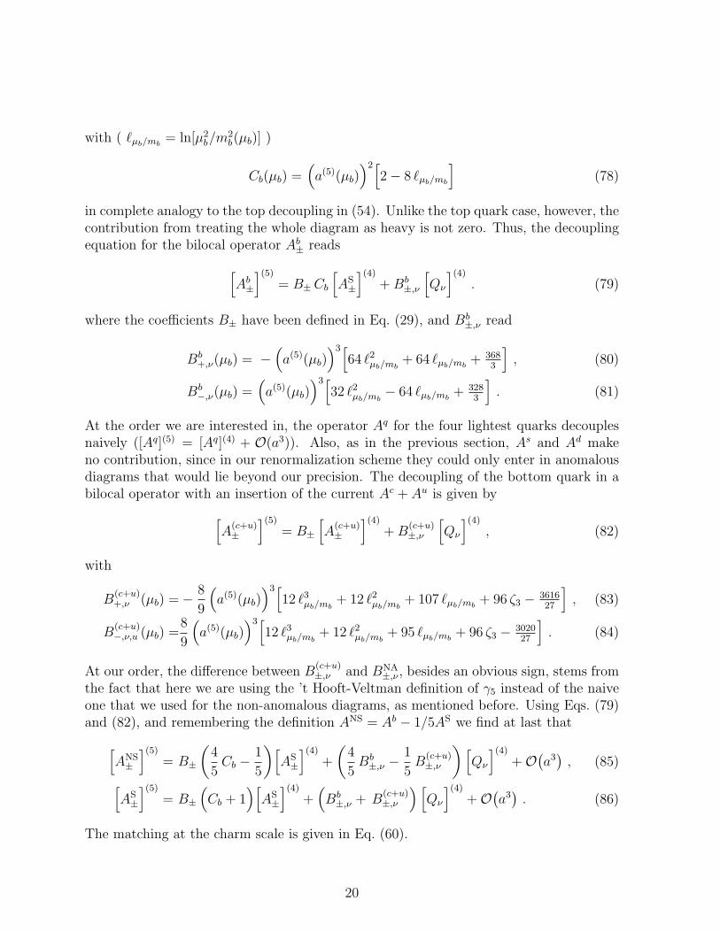
We observe that the anomalous contributions, dominated by XW,b, are two ordersof magnitude smaller than the non-anomalous ones, and the uncertainty of the lattermakes them completely negligible. Indeed, the uncertainties in for XNA and XW,b are ofa remarkable size. In Figure 12 we show the relative uncertainties of XNA and XW,t+b

at each order, that is δXNALO /|XNA

LO |, δ(XNALO + XNA

NLO)/|XNALO + XNA

NLO)| and so on. Aswe can see, δXNA is completely dominated by the µc dependence, δXNA

µc, which grows

substantially in relative size at NLO, and keeps growing at NNLO. In the case of XW,t+b

the µc dependence still dominates and grows, although not to the same degree as in thenon-anomalous case.

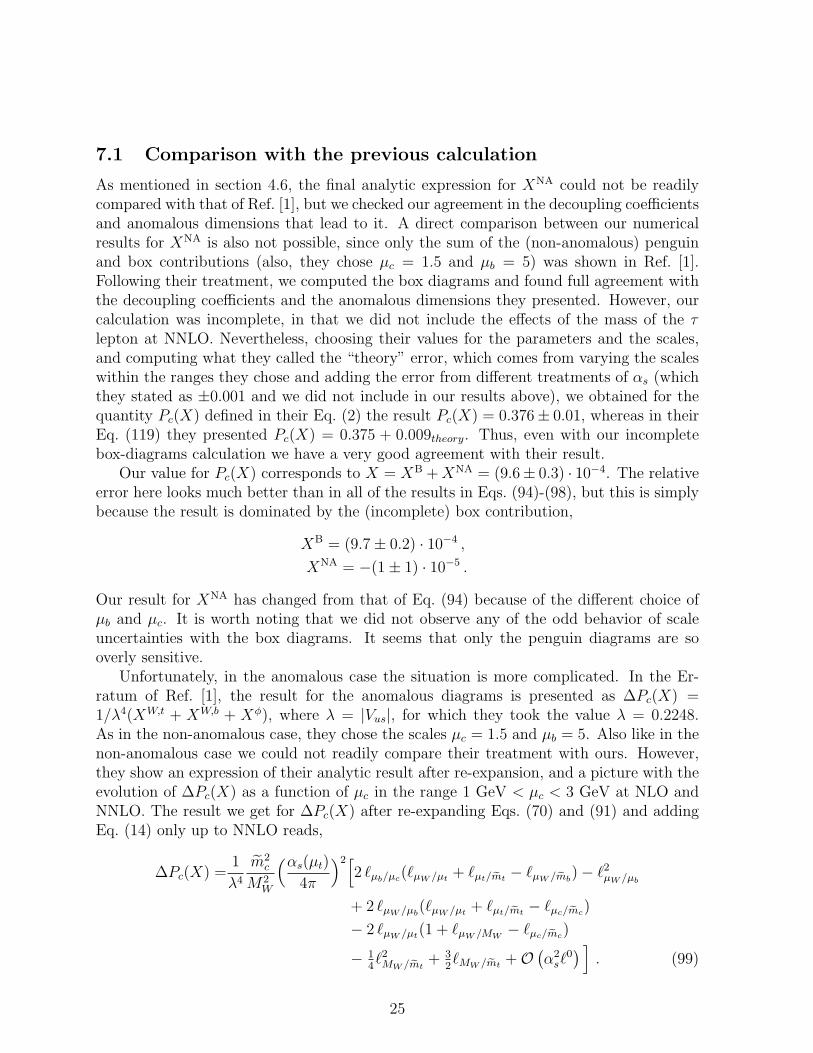
We observe uncertainties in the pictures growing when moving from one order to thenext. This was unexpected, as normally uncertainties should diminish when increasingthe order of our calculation. This odd increase in µ dependence, and the dominanceof δXµc especially in the non-anomalous case, seem to indicate that there might be aproblem with the perturbation series, and that it might stem from the size of αs(µc). Atµ = 3GeV, we have that αs ' 0.252.

We test this in two ways. First, we artificially set αs(MZ) = 0.097, which leads toαs(3GeV)' 0.170. Second, we artificially increase the mass of the charm quark, setting it

23

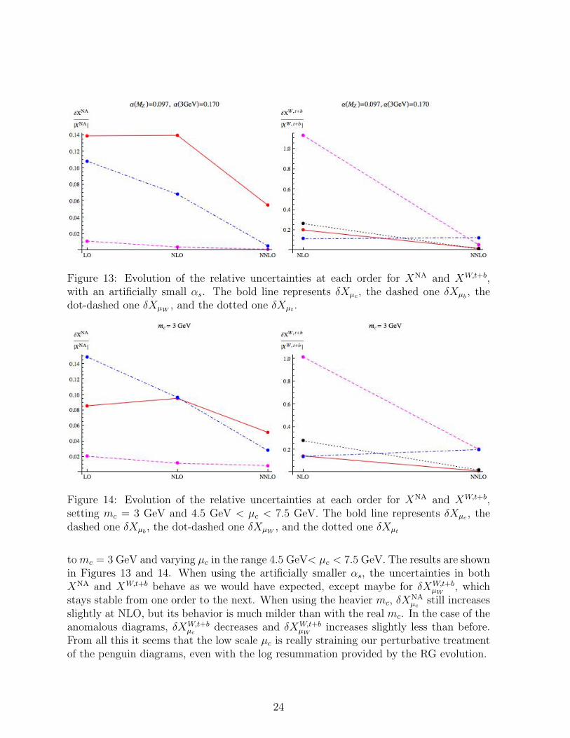
Figure 13: Evolution of the relative uncertainties at each order for XNA and XW,t+b,with an artificially small αs. The bold line represents δXµc , the dashed one δXµb

, thedot-dashed one δXµW

, and the dotted one δXµt .

Figure 14: Evolution of the relative uncertainties at each order for XNA and XW,t+b,setting mc = 3 GeV and 4.5 GeV < µc < 7.5 GeV. The bold line represents δXµc , thedashed one δXµb

, the dot-dashed one δXµW, and the dotted one δXµt

tomc = 3 GeV and varying µc in the range 4.5 GeV< µc < 7.5 GeV. The results are shownin Figures 13 and 14. When using the artificially smaller αs, the uncertainties in bothXNA and XW,t+b behave as we would have expected, except maybe for δXW,t+b

µW, which

stays stable from one order to the next. When using the heavier mc, δXNAµc

still increasesslightly at NLO, but its behavior is much milder than with the real mc. In the case of theanomalous diagrams, δXW,t+b

µcdecreases and δXW,t+b

µWincreases slightly less than before.

From all this it seems that the low scale µc is really straining our perturbative treatmentof the penguin diagrams, even with the log resummation provided by the RG evolution.

24

7.1 Comparison with the previous calculation

As mentioned in section 4.6, the final analytic expression for XNA could not be readilycompared with that of Ref. [1], but we checked our agreement in the decoupling coefficientsand anomalous dimensions that lead to it. A direct comparison between our numericalresults for XNA is also not possible, since only the sum of the (non-anomalous) penguinand box contributions (also, they chose µc = 1.5 and µb = 5) was shown in Ref. [1].Following their treatment, we computed the box diagrams and found full agreement withthe decoupling coefficients and the anomalous dimensions they presented. However, ourcalculation was incomplete, in that we did not include the effects of the mass of the τlepton at NNLO. Nevertheless, choosing their values for the parameters and the scales,and computing what they called the “theory” error, which comes from varying the scaleswithin the ranges they chose and adding the error from different treatments of αs (whichthey stated as ±0.001 and we did not include in our results above), we obtained for thequantity Pc(X) defined in their Eq. (2) the result Pc(X) = 0.376± 0.01, whereas in theirEq. (119) they presented Pc(X) = 0.375 + 0.009theory. Thus, even with our incompletebox-diagrams calculation we have a very good agreement with their result.

Our value for Pc(X) corresponds to X = XB +XNA = (9.6± 0.3) · 10−4. The relativeerror here looks much better than in all of the results in Eqs. (94)-(98), but this is simplybecause the result is dominated by the (incomplete) box contribution,

XB = (9.7± 0.2) · 10−4 ,

XNA = −(1± 1) · 10−5 .

Our result for XNA has changed from that of Eq. (94) because of the different choice ofµb and µc. It is worth noting that we did not observe any of the odd behavior of scaleuncertainties with the box diagrams. It seems that only the penguin diagrams are sooverly sensitive.

Unfortunately, in the anomalous case the situation is more complicated. In the Er-ratum of Ref. [1], the result for the anomalous diagrams is presented as ∆Pc(X) =1/λ4(XW,t + XW,b + Xφ), where λ = |Vus|, for which they took the value λ = 0.2248.As in the non-anomalous case, they chose the scales µc = 1.5 and µb = 5. Also like in thenon-anomalous case we could not readily compare their treatment with ours. However,they show an expression of their analytic result after re-expansion, and a picture with theevolution of ∆Pc(X) as a function of µc in the range 1 GeV < µc < 3 GeV at NLO andNNLO. The result we get for ∆Pc(X) after re-expanding Eqs. (70) and (91) and addingEq. (14) only up to NNLO reads,

∆Pc(X) =1

λ4

m2c

M2W

(αs(µt)4π

)2[2 `µb/µc(`µW /µt + `µt/emt − `µW /emb

)− `2µW /µb

+ 2 `µW /µb(`µW /µt + `µt/emt − `µc/emc)

− 2 `µW /µt(1 + `µW /MW− `µc/emc)

− 14`2MW /emt

+ 32`MW /emt +O

(α2s`

0) ]

. (99)

25

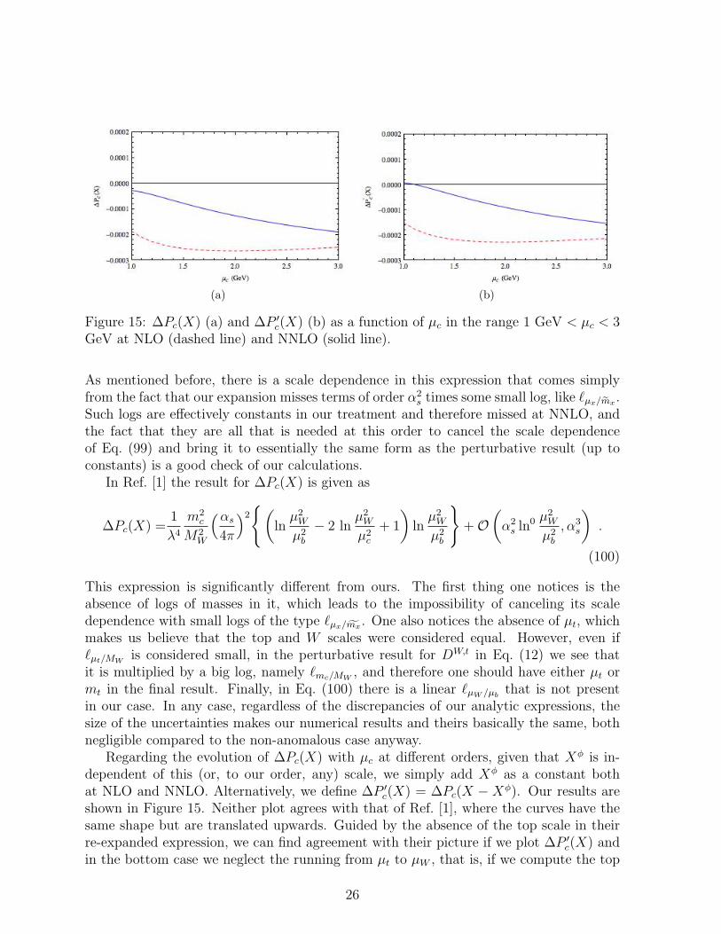
(a) (b)

Figure 15: ∆Pc(X) (a) and ∆P ′c(X) (b) as a function of µc in the range 1 GeV < µc < 3

GeV at NLO (dashed line) and NNLO (solid line).

As mentioned before, there is a scale dependence in this expression that comes simplyfrom the fact that our expansion misses terms of order α2

s times some small log, like `µx/emx .Such logs are effectively constants in our treatment and therefore missed at NNLO, andthe fact that they are all that is needed at this order to cancel the scale dependenceof Eq. (99) and bring it to essentially the same form as the perturbative result (up toconstants) is a good check of our calculations.

In Ref. [1] the result for ∆Pc(X) is given as

∆Pc(X) =1

λ4

m2c

M2W

(αs4π

)2{(

lnµ2W

µ2b

− 2 lnµ2W

µ2c

+ 1

)lnµ2W

µ2b

}+O

(α2s ln0 µ

2W

µ2b

, α3s

).

(100)

This expression is significantly different from ours. The first thing one notices is theabsence of logs of masses in it, which leads to the impossibility of canceling its scaledependence with small logs of the type `µx/fmx . One also notices the absence of µt, whichmakes us believe that the top and W scales were considered equal. However, even if`µt/MW

is considered small, in the perturbative result for DW,t in Eq. (12) we see thatit is multiplied by a big log, namely `mc/MW

, and therefore one should have either µt ormt in the final result. Finally, in Eq. (100) there is a linear `µW /µb

that is not presentin our case. In any case, regardless of the discrepancies of our analytic expressions, thesize of the uncertainties makes our numerical results and theirs basically the same, bothnegligible compared to the non-anomalous case anyway.

Regarding the evolution of ∆Pc(X) with µc at different orders, given that Xφ is in-dependent of this (or, to our order, any) scale, we simply add Xφ as a constant bothat NLO and NNLO. Alternatively, we define ∆P ′

c(X) = ∆Pc(X − Xφ). Our results areshown in Figure 15. Neither plot agrees with that of Ref. [1], where the curves have thesame shape but are translated upwards. Guided by the absence of the top scale in theirre-expanded expression, we can find agreement with their picture if we plot ∆P ′

c(X) andin the bottom case we neglect the running from µt to µW , that is, if we compute the top

26

case starting from µt and the bottom case starting from µW . This produces essentiallythe same results within the errors, but as mentioned before it produces an unbalanced µtdependence which was not present in the original perturbative diagrams.

8 Conclusion

In this paper we set out to check the results for penguin-type charm contributions to thedecay K+ → π+νν presented in Ref. [1]. It is quite an involved calculation, certainlydeserving an independent check. We have found full agreement for all the decouplingcoefficients and anomalous dimensions for the non-anomalous diagrams. In Ref. [1] thefinal numerical result presented was the sum of non-anomalous penguin and box-typediagrams, so in order to perform a comparison we also had to compute the latter. Ourcalculation missed τ -mass effects, but again we confirmed the corresponding decouplingcoefficients and anomalous dimensions presented in Ref. [1]. Incomplete as our result forthe box diagrams was, it was enough to allow us to obtain very good agreement in the finalnumerical result, both in the central value and the estimate of theoretical uncertainty.

We found some discrepancies with Ref. [1] in our results for the anomalous diagrams.Although numerically the differences get washed out by the uncertainty (and by the sheersmallness of the anomalous contributions versus the non-anomalous ones), the analyticexpression of our re-expanded result differs significantly from that of Ref. [1].

Our results show some unstable behavior and quite a large uncertainty. The causeseems to be the low scale µc, which might be testing the limits of perturbation theory.This only applies to the penguin diagrams, however, as in our evaluation of the boxdiagrams the scale uncertainties behaved as expected, diminishing at each order andremaining relatively small. We were not able to find an analytic reason for the uniqueunstable behavior of the penguin diagrams.

Acknowledgments. We are grateful to K.G. Chetyrkin for his invaluable help andsupport throughout this project. We also wish to thank A. Buras, M. Gorbahn, U. Haisch,and U. Nierste for helpful discussions and for sharing their Erratum with us prior topublication. This work was supported by the Deutsche Forschungsgemeinschaft in theSonderforschungsbereich/Transregio SFB/TR9 “Computational Particle Physics”.

A Definition of the evanescent operators

In dimensional regularization the operators Qq± introduced in Eq. (20) are not enough to

perform the decoupling of the W boson in the subdiagram shown in Figure 9b. A setof evanescent operators (vanishing at d = 4) is required. In our renormalization schemethese operators have vanishing matrix elements, but they still contribute by determiningthe anomalous dimensions of Qq

±. Since we reach O(α2s) in our calculations, we need six

evanescent operators. We take the definitions from Ref. [1], with a different normalization

27

factor, coming from using a (V − A) current instead of left-handed fields. If we define

Qq1 =

(sγµ(1− γ5)t

aq)(qγµ(1− γ5)t

ad)

(101)

Qq2 =

(sγµ(1− γ5)q

)(qγµ(1− γ5)d

), (102)

where ta is a generator of the color group, then one can define the following evanescentoperators,

Eq1 =

(sγµ1µ2µ3(1− γ5)t

aq)(qγµ1µ2µ3(1− γ5)t

ad)− (16− 4ε− 4ε2)Qq

1 , (103)

Eq2 =

(sγµ1µ2µ3(1− γ5)q

)(qγµ1µ2µ3(1− γ5)d

)− (16− 4ε− 4ε2)Qq

2 , (104)

Eq3 =

(sγµ1µ2µ3µ4µ5(1− γ5)t

aq)(qγµ1µ2µ3µ4µ5(1− γ5)t

ad)

−(256− 224ε− 571225ε2)Qq

1 , (105)

Eq4 =

(sγµ1µ2µ3µ4µ5(1− γ5)q

)(qγµ1µ2µ3µ4µ5(1− γ5)d

)−(256− 224ε− 10032

25ε2)Qq

2 , (106)

Eq5 =

(sγµ1µ2µ3µ4µ5µ6µ7(1− γ5)t

aq)(qγµ1µ2µ3µ4µ5µ6µ7(1− γ5)t

ad)

−(4096− 7680ε)Qq1 , (107)

Eq6 =

(sγµ1µ2µ3µ4µ5µ6µ7(1− γ5)q

)(qγµ1µ2µ3µ4µ5µ6µ7(1− γ5)d

)−(4096− 7680ε−)Qq

2 . (108)

Here the notation γµ1µ2...µn = γµ1γµ2 . . . γµn has been used. The operators Qq1,2 are com-

bined to produce Qq± in the following way,

Qq+ = Q1 +

nc + 1

2ncQ2 , (109)

Qq− = −Q1 +

nc − 1

2ncQ2 , (110)

where nc is the number of colors. In the same way, the pairs (Eq3 , E

q4) and (Eq

5 , Eq6) are

combined to generate E± operators, which are the ones we use. The above definitions ofthe evanescent operators ensure that Qq

± do not mix with each other through NNLO.

References

[1] A. J. Buras, M. Gorbahn, U. Haisch, and U. Nierste, Charm Quark Contribution toK+ → pi+ nu anti-nu at Next- to-Next-to-Leading Order, JHEP 11 (2006) 002,[hep-ph/0603079].

[2] A. I. Vainshtein, V. I. Zakharov, V. A. Novikov, and M. A. Shifman, On the StrongInteraction Effects on the K(L) → 2 mu Decay and K(L) K(s) Mass Difference. AReply, Phys. Rev. D16 (1977) 223.

[3] J. R. Ellis and J. S. Hagelin, Constraints on Light Particles from Kaon Decays,Nucl. Phys. B217 (1983) 189.

28

[4] C. Dib, I. Dunietz, and F. J. Gilman, STRONG INTERACTION CORRECTIONSTO THE DECAY K → pi neutrino anti-neutrino FOR LARGE m(t), Mod. Phys.Lett. A6 (1991) 3573–3582.

[5] G. Buchalla and A. J. Buras, QCD corrections to rare K and B decays for arbitrarytop quark mass, Nucl. Phys. B400 (1993) 225–239.

[6] M. Misiak and J. Urban, QCD corrections to FCNC decays mediated by Z-penguinsand W-boxes, Phys. Lett. B451 (1999) 161–169, [hep-ph/9901278].

[7] G. Buchalla and A. J. Buras, The rare decays K+ → pi+ neutrino anti-neutrinoand K(L) → mu+ mu- beyond leading logarithms, Nucl. Phys. B412 (1994)106–142, [hep-ph/9308272].

[8] G. Buchalla and A. J. Buras, The rare decays K → pi nu anti-nu, B → X nuanti-nu and B → l+ l-: An update, Nucl. Phys. B548 (1999) 309–327,[hep-ph/9901288].

[9] A. J. Buras, Minimal flavor violation, Acta Phys.Polon. B34 (2003) 5615–5668,[hep-ph/0310208].

[10] A. J. Buras, Flavor physics and CP violation, hep-ph/0505175.

[11] A. J. Buras, Waiting for clear signals of new physics in B and K decays, SpringerProc.Phys. 98 (2005) 315–331, [hep-ph/0402191].

[12] A. Buras, P. Gambino, M. Gorbahn, S. Jager, and L. Silvestrini, Universal unitaritytriangle and physics beyond the standard model, Phys.Lett. B500 (2001) 161–167,[hep-ph/0007085].

[13] G. D’Ambrosio and G. Isidori, K+ → pi+ nu anti-nu: A Rising star on the stage offlavor physics, Phys.Lett. B530 (2002) 108–116, [hep-ph/0112135].

[14] A. J. Buras, F. Schwab, and S. Uhlig, Waiting for precise measurements of K+ →pi+ nu anti-nu and K(L) → pi0 nu anti-nu, Rev. Mod. Phys. 80 (2008) 965–1007,[hep-ph/0405132].

[15] W. J. Marciano and Z. Parsa, Rare kaon decays with ’missing energy’, Phys. Rev.D53 (1996) 1–5.

[16] G. Isidori, F. Mescia, and C. Smith, Light-quark loops in K → pi nu nu, Nucl.Phys. B718 (2005) 319–338, [hep-ph/0503107].

[17] G. Isidori, G. Martinelli, and P. Turchetti, Rare kaon decays on the lattice, Phys.Lett. B633 (2006) 75–83, [hep-lat/0506026].

[18] J. C. Collins, F. Wilczek, and A. Zee, Low-Energy Manifestations of HeavyParticles: Application to the Neutral Current, Phys.Rev. D18 (1978) 242.

29

[19] K. Chetyrkin and J. H. Kuhn, Neutral current in the heavy top quark limit and therenormalization of the singlet axial current, Z.Phys. C60 (1993) 497–502.

[20] G. ’t Hooft and M. Veltman, Regularization and Renormalization of Gauge Fields,Nucl.Phys. B44 (1972) 189–213.

[21] S. A. Larin, The Renormalization of the axial anomaly in dimensionalregularization, Phys. Lett. B303 (1993) 113–118, [hep-ph/9302240].

[22] M. B. Voloshin, K(L) → mu+ mu- Decay and (n Lambda Z) Vertex in theWeinberg-Salam Model, Sov. J. Nucl. Phys. 24 (1976) 422–426.[Yad.Fiz.24:810-819,1976].

[23] G. Buchalla and A. J. Buras, QCD corrections to the anti-s d Z vertex for arbitrarytop quark mass, Nucl. Phys. B398 (1993) 285–300.

[24] M. Misiak and M. Steinhauser, Three-loop matching of the dipole operators for b →s gamma and b → s g, Nucl. Phys. B683 (2004) 277–305, [hep-ph/0401041].

[25] P. Nogueira, Automatic Feynman graph generation, J. Comput. Phys. 105 (1993)279–289.

[26] R. Harlander, T. Seidensticker, and M. Steinhauser, Complete corrections ofO(alpha alpha(s)) to the decay of the Z boson into bottom quarks, Phys. Lett. B426(1998) 125–132, [hep-ph/9712228].

[27] T. Seidensticker, Automatic application of successive asymptotic expansions ofFeynman diagrams, hep-ph/9905298.

[28] J. A. M. Vermaseren, New features of FORM, math-ph/0010025.

[29] M. Steinhauser, MATAD: A program package for the computation of massivetadpoles, Comput. Phys. Commun. 134 (2001) 335–364, [hep-ph/0009029].

[30] K. G. Chetyrkin, B. A. Kniehl, and M. Steinhauser, Decoupling relations toO(alpha(s)**3) and their connection to low-energy theorems, Nucl. Phys. B510(1998) 61–87, [hep-ph/9708255].

[31] M. J. Dugan and B. Grinstein, On the vanishing of evanescent operators, Phys.Lett. B256 (1991) 239–244.

[32] K. G. Chetyrkin and J. H. Kuhn, Complete QCD corrections of order alpha-s**2 tothe Z decay rate, Phys. Lett. B308 (1993) 127–136.

[33] K. Chetyrkin, J. H. Kuhn, and M. Steinhauser, RunDec: A Mathematica packagefor running and decoupling of the strong coupling and quark masses,Comput.Phys.Commun. 133 (2000) 43–65, [hep-ph/0004189].

30