ON CLUSTERING FINANCIAL TIME SERIESGAUTIER MARTI, PHILIPPE DONNAT AND FRANK NIELSEN

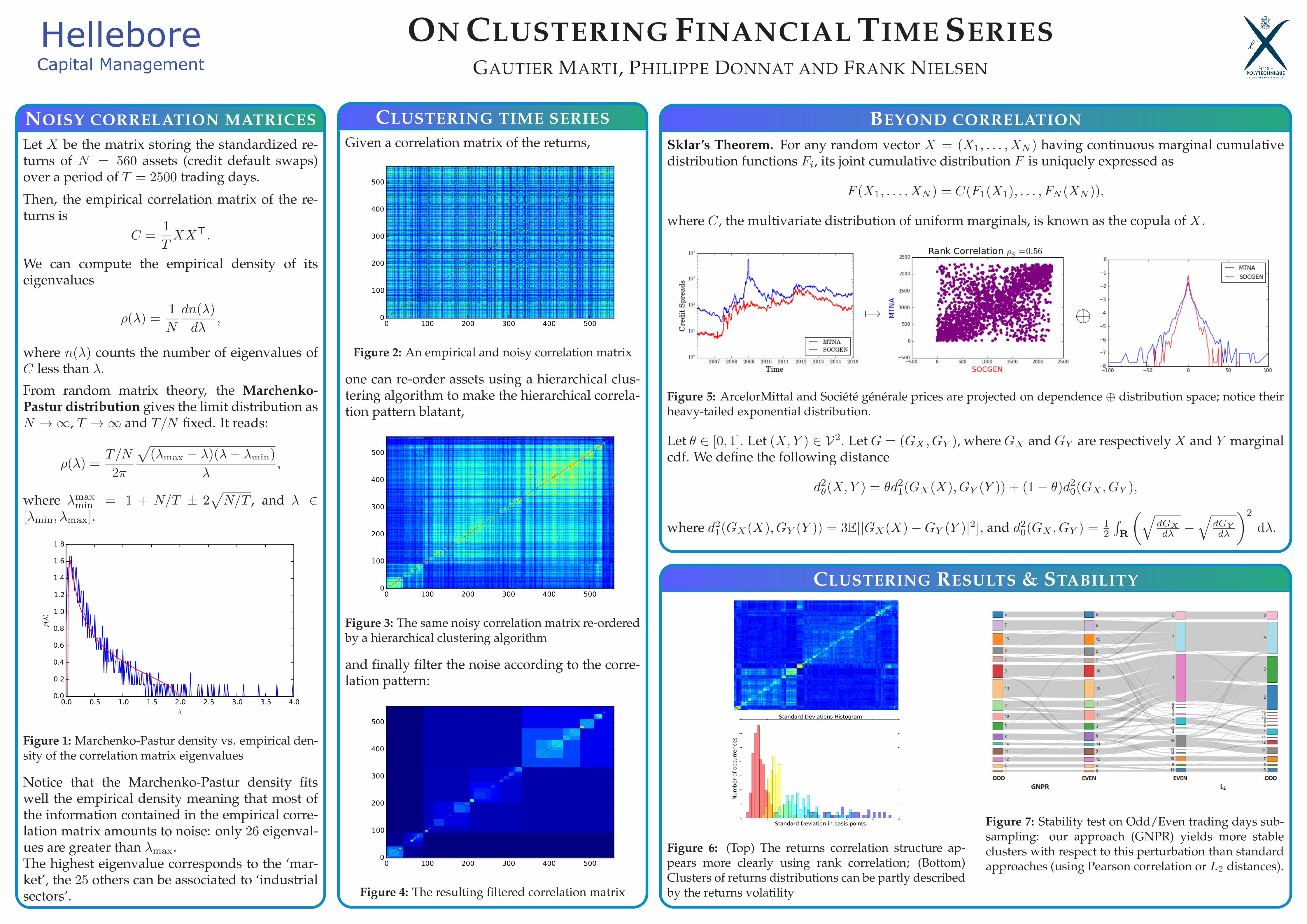
NOISY CORRELATION MATRICESLet X be the matrix storing the standardized re-turns of N = 560 assets (credit default swaps)over a period of T = 2500 trading days.

Then, the empirical correlation matrix of the re-turns is

C =1

TXX>.

We can compute the empirical density of itseigenvalues

ρ(λ) =1

N

dn(λ)

dλ,

where n(λ) counts the number of eigenvalues ofC less than λ.

From random matrix theory, the Marchenko-Pastur distribution gives the limit distribution asN →∞, T →∞ and T/N fixed. It reads:

ρ(λ) =T/N

2π

√(λmax − λ)(λ− λmin)

λ,

where λmaxmin = 1 + N/T ± 2

√N/T , and λ ∈

[λmin, λmax].

0.0 0.5 1.0 1.5 2.0 2.5 3.0 3.5 4.0

λ

0.0

0.2

0.4

0.6

0.8

1.0

1.2

1.4

1.6

1.8

ρ(λ

)

Figure 1: Marchenko-Pastur density vs. empirical den-sity of the correlation matrix eigenvalues

Notice that the Marchenko-Pastur density fitswell the empirical density meaning that most ofthe information contained in the empirical corre-lation matrix amounts to noise: only 26 eigenval-ues are greater than λmax.The highest eigenvalue corresponds to the ‘mar-ket’, the 25 others can be associated to ‘industrialsectors’.

CLUSTERING TIME SERIESGiven a correlation matrix of the returns,

0 100 200 300 400 5000

100

200

300

400

500

Figure 2: An empirical and noisy correlation matrix

one can re-order assets using a hierarchical clus-tering algorithm to make the hierarchical correla-tion pattern blatant,

0 100 200 300 400 5000

100

200

300

400

500

Figure 3: The same noisy correlation matrix re-orderedby a hierarchical clustering algorithm

and finally filter the noise according to the corre-lation pattern:

0 100 200 300 400 5000

100

200

300

400

500

Figure 4: The resulting filtered correlation matrix

BEYOND CORRELATIONSklar’s Theorem. For any random vector X = (X1, . . . , XN ) having continuous marginal cumulativedistribution functions Fi, its joint cumulative distribution F is uniquely expressed as

F (X1, . . . , XN ) = C(F1(X1), . . . , FN (XN )),

where C, the multivariate distribution of uniform marginals, is known as the copula of X .

Figure 5: ArcelorMittal and Société générale prices are projected on dependence ⊕ distribution space; notice theirheavy-tailed exponential distribution.

Let θ ∈ [0, 1]. Let (X,Y ) ∈ V2. Let G = (GX , GY ), where GX and GY are respectively X and Y marginalcdf. We define the following distance

d2θ(X,Y ) = θd21(GX(X), GY (Y )) + (1− θ)d20(GX , GY ),

where d21(GX(X), GY (Y )) = 3E[|GX(X)−GY (Y )|2], and d20(GX , GY ) =12

∫R

(√dGX

dλ −√

dGY

dλ

)2

dλ.

CLUSTERING RESULTS & STABILITY

0 5 10 15 20 25 30

Standard Deviation in basis points0

5

10

15

20

25

30

35

Num

ber

of

occ

urr

ence

s

Standard Deviations Histogram

Figure 6: (Top) The returns correlation structure ap-pears more clearly using rank correlation; (Bottom)Clusters of returns distributions can be partly describedby the returns volatility

Figure 7: Stability test on Odd/Even trading days sub-sampling: our approach (GNPR) yields more stableclusters with respect to this perturbation than standardapproaches (using Pearson correlation or L2 distances).