Numerical modeling and analysis of early shock wave

interactions with a dense particle cloud

J. D. Regele∗, J. Rabinovitch, T. Colonius, and G. Blanquart†

California Institute of Technology, Pasadena, CA, 91125, U.S.A.

Dense compressible multiphase flows exist in variable phase turbines, explosions, andfluidized beds, where the particle volume fraction is in the range 0.001 < αd < 0.5. Asimple model problem that can be used to study modeling issues related to these typesof flows is a shock wave impacting a particle cloud. In order to characterize the initialshock-particle interactions when there is little particle movement, a two-dimensional (2-D)model problem is created where the particles are frozen in place. Qualitative comparisonwith experimental data indicates that the 2-D model captures the essential flow physics.Volume-averaging of the 2-D data is used to reduce the data to one dimension, and x-tdiagrams are used to characterize the flow behavior. An equivalent one-dimensional (1-D)model problem is developed for direct comparison with the 2-D model. While the 1-Dmodel characterizes the overall steady-state flow behavior well, it fails to capture aspectsof the unsteady behavior. As might be expected, it is found that neglecting the unclosedfluctuation terms inherent in the volume-averaged equations is not appropriate for densegas-particle flows.

Nomenclature

α Volume fractionρ Phase-averaged gas phase densityp Phase-averaged pressureu Mass-averaged gas phase velocityeT Phase-averaged total energyhT Phase-averaged total enthalpyFD Drag force on a single particlen Number densityAp Particle Cross-sectional areaDp Particle diameterx Nondimensional positiont Nondimensional timeVp Particle volume

Subscriptc Continuous phased Disperse phase0 Reference statep ParticleSuperscript′ Dimensioned quantity

∗Postdoctoral scholar, Department of Mechanical Engineering; jonathan.regele@caltech.edu. AIAA Member.†Assistant Professor, Department of Mechanical Engineering; g.blanquart@caltech.edu. AIAA Member.

1 of 14

American Institute of Aeronautics and Astronautics

42nd AIAA Fluid Dynamics Conference and Exhibit25 - 28 June 2012, New Orleans, Louisiana

AIAA 2012-3161

Copyright © 2012 by Jonathan Regele. Published by the American Institute of Aeronautics and Astronautics, Inc., with permission.

Dow

nloa

ded

by G

uilla

ume

Bla

nqua

rt o

n Ju

ly 3

1, 2

015

| http

://ar

c.ai

aa.o

rg |

DO

I: 1

0.25

14/6

.201

2-31

61

I. Introduction

Dense multiphase flows can be found in a variety of practical applications, including fluidized beds,variable phase turbines, and explosions. Variable phase turbines can be used in waste-heat recovery andgeothermal power generation, but their efficiency is limited by the accuracy of modeling approaches used inthe design phase. The ability to design a turbine accurately is dependent upon predicting mass, momentum,and energy transfer between phases as well as droplet formation, breakup, and collisions. Current state ofthe art models are often inadequate, and designers still rely heavily on experimental testing. Other fields,such as fluidized beds and explosives, suffer from similar modeling deficiencies.

Multiphase flow behavior can be divided into three main categories: dilute flow where the particle volumefraction is αd < 0.001, collision-dominated flows where 0.001 < αd < 0.1, and contact-dominated flows withαd > 0.1.1 Contrary to the former definition, the transition from collision dominated to contact dominatedflow is defined differently in Ref. 2. They consider the transition to occur when the particle density is highenough that the disperse phase becomes a packed bed (αd > 0.5) and the flow can be considered granular.In dilute flows, collisions can essentially be neglected.1 In granular flows, particles are packed together suchthat particle motion is induced by direct inter-particle forces and gas propagation through the porous regionbetween particles. Between these two limiting extremes lies gas-solid two-phase flow, where particle collisionsand fluid drag both play major roles in flow behavior.

Drag coefficient correlations have been developed for dilute flows.3 However, for larger disperse phasevolume fraction, the steady-state drag coefficient, CD, deviates from the standard drag curve values.4,5, 6

Consequently, voidage functions have been developed to modify the drag coefficient to account for thisdependency, such that CD = CD0g(αc), where g(αc) is the voidage function and CD0 is the drag coefficientof a single particle.4,5, 7 However, these formulations have been developed for low Mach number flows wherecompressibility effects can be neglected. It is unclear how accurate they will be at capturing the dragcoefficient in dense compressible multiphase flows.

A shock wave impacting a cloud of particles is a model problem that can be used to study shock-particle interactions and compressible multiphase flows. A combination of both experiments and numericalsimulations have been used already to describe the response of a shock wave impacting dilute/dusty particleclouds .8,9, 10,11,12

In the dilute regime, these flows are well characterized. In the granular regime where the particles aredensely packed, continuum mixture theories exist to describe these flows.13,14 Baer15 successfully modelednormal shock impingement experiments of Anderson, Graham, and Holman16 and Sommerfeld.17 Betweenthese two limiting flow regimes, little information exists for gas-solid flows where the volume fraction isin the range 0.001 < αd < 0.5. Boiko et al.18 performed experiments of shock waves impacting spatiallyinhomogeneous particle clouds in the range 0.001 < αd < 0.03. In the case where αd = 0.03, a reflectedshock wave was observed, whereas in the more dilute cases no reflected shock was observed.

Recently, a multiphase shock tube experiment has been developed at Sandia National Labs.19,20 In thisexperiment, a shock wave (M = 1.67) impinges on a gravity fed particle cloud of width L′ = 3.2mm. Theparticle volume fraction inside the cloud is approximately αd = 0.15 to 0.2 and the particles are of nearlyuniform diameter. Detailed Schlieren images show the fluid response to the impact with the particle cloud.Reflected and transmitted shock waves are observed from the shock wave interaction with the cloud. Forthe first 30μs, the cloud does not move, but after a few hundred microseconds, the trailing edge of the cloudtravels several cloud lengths downstream, while the leading edge moves much less.

It is unclear what occurs when a shock wave impacts a dense particle field, particularly inside and justbehind the particle cloud. The amount of information that can be obtained inside the cloud experimentallyis limited. The goal of the present work is to perform a detailed investigation of the interaction betweenthe incident shock wave and the particle cloud during the first several microseconds. Individual objectivesof the current work are to a) develop an equivalent two-dimensional (2-D) model problem that capturesthe essential physics in this experiment, b) perform detailed 2-D numerical simulations of a shock waveimpinging upon a cloud in order to characterize the flow behavior, c) compare the results with experimentaldata for qualitative consistency, d) perform one-dimensional (1-D) simulations using a standard volumefraction approach, and e) compare the two different model results and identify what details are captured andmissing in the one-dimensional model. The present analysis is limited to the early “time” when the particleshave not moved yet due to drag forces and can be assumed to be frozen in place.

The paper is organized as follows. First, a mathematical model is developed to describe the shockinteraction behavior with a 2-D particle cloud. Then, results of the 2-D model and a discussion of the

2 of 14

American Institute of Aeronautics and Astronautics

Dow

nloa

ded

by G

uilla

ume

Bla

nqua

rt o

n Ju

ly 3

1, 2

015

| http

://ar

c.ai

aa.o

rg |

DO

I: 1

0.25

14/6

.201

2-31

61

multidimensional effects and grid independence are presented in Section III. A 1-D volume-averaged modelfor direct comparison with the 2-D model is developed in Section IV. In Section V, the flow behavior isgeneralized, similarities and differences between the two models are highlighted, and additional terms thatneed to be modeled are identified. The paper concludes with a discussion of the current numerical resultswith the experimental data in Ref. 20.

II. Mathematical Model

The current work attempts to capture qualitatively the effects of a shock wave interacting with a cloudof spherical particles using a two-dimensional model. The Reynolds number based on the velocity behindthe reflected shock and the particle diameter is approximately Re = 2000.20 Hence, the viscous forces onthe particles are expected to be negligible, and the drag force on a particle is predominantly from drag.

The current work is focused on the initial transient interactions between the incident shock wave andthe particle cloud. In the experiments in Ref. 20, this coincides with approximately the first 30-50μs.Experimental data during this time shows little, if any, particle movement,20,18,21 which makes it reasonableto assume that the particles are frozen in place. Furthermore, heat transfer can be neglected over such ashort time frame. Finally, the particles are solid so there is no mass exchange between phases.

II.A. Representation of particle cloud

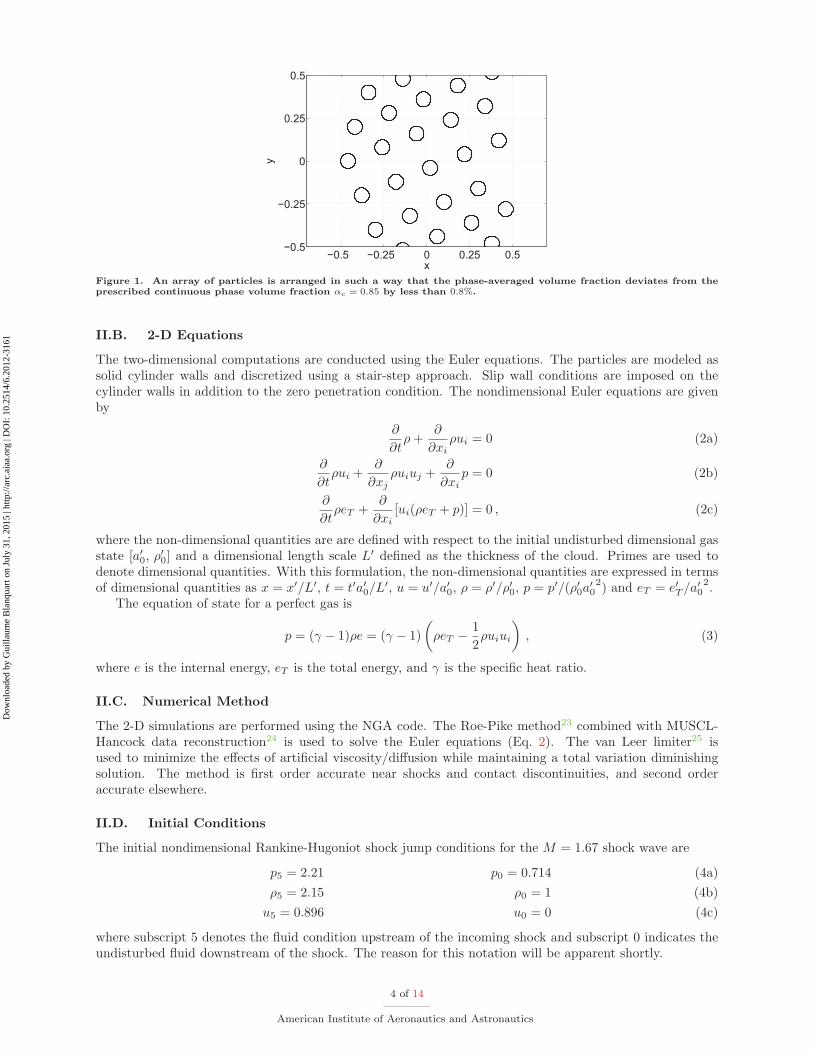
Clemins22 demonstrated that to maintain small volume fraction fluctuations, 〈α〉 − α (where 〈α〉 is thevolume average over a given sample volume and α is the expected volume fraction), at least 60-150 particlesare required inside of a 3-D sampling volume. Following his 3-D analysis, we estimate that between 15 and30 particles should be sufficient in our 2-D simulations. The 2-D particle cloud is modeled using a staggeredparticle matrix with a total of 24 particles (approximately 5 particles in each direction). Figure 1 shows thearrangement of the particles for the two-dimensional simulations. By staggering each particle both in thex- and y-directions with equal spacing, a relatively small number of particles can be used and still maintainsmall fluctuations, less than ‖〈αd〉 − αd‖∞ < 0.008. The sampling volume used to determine 〈αd〉 spansthe entire cloud height in the y-direction, and a distance Dp/2 in the horizontal direction, where Dp is theparticle diameter.

The particle diameter inside the cloud is related to the expected particle volume fraction, which is chosento be αd = 0.15. In the 2-D model, the volume fraction is expressed as an area fraction by

αd =NπD2

p

4L2. (1)

Here, N is the total number of particles inside the square cloud of nondimensional length L and area/volumefraction αd = 0.15. Since the length scale is nondimensionalized with respect to the cloud length (L = 1),the particle diameter is Dp = 0.089 for N = 24 particles. A full discussion of the nondimensionalization ispresented in the next section.

The cloud is located between x = −0.5 and 0.5, and the computational domain spans the range x ∈[−2.5, 3.5] and y ∈ [−0.5, 0.5]. Inflow and outflow conditions are used on the left and right boundaries,respectively, and the top and bottom boundaries are periodic to simulate an infinitely tall cloud. Thesimulation uses a cartesian grid. The grid spacing is uniform in the y-direction and in the x-direction forx ∈ [−1.5, 1.5]. In this region, the cells have unity aspect ratio, Δx = Δy. Outside of this range, unequalspacing is used in the x-direction.

Simulations were performed for four different levels of resolution to determine grid sensitivity. Thenumber of cells used to resolve the particles in the four different cases were 13, 26, 52, and 105 cells perparticle.

It should be reiterated that the two-dimensional model described above is not intended to provide aquantitatively accurate comparison with experimental data.20 The current motivation is to capture qualita-tively the essential physics in two dimensions and use the volume-averaged solution to determine what the1-D model is capable of capturing and what needs to be modeled. Full three-dimensional simulations forquantitative comparison with experimental data will be the subject of future work.

3 of 14

American Institute of Aeronautics and Astronautics

Dow

nloa

ded

by G

uilla

ume

Bla

nqua

rt o

n Ju

ly 3

1, 2

015

| http

://ar

c.ai

aa.o

rg |

DO

I: 1

0.25

14/6

.201

2-31

61

xy

−0.5 −0.25 0 0.25 0.5−0.5

−0.25

0

0.25

0.5

Figure 1. An array of particles is arranged in such a way that the phase-averaged volume fraction deviates from theprescribed continuous phase volume fraction αc = 0.85 by less than 0.8%.

II.B. 2-D Equations

The two-dimensional computations are conducted using the Euler equations. The particles are modeled assolid cylinder walls and discretized using a stair-step approach. Slip wall conditions are imposed on thecylinder walls in addition to the zero penetration condition. The nondimensional Euler equations are givenby

∂

∂tρ+

∂

∂xiρui = 0 (2a)

∂

∂tρui +

∂

∂xjρuiuj +

∂

∂xip = 0 (2b)

∂

∂tρeT +

∂

∂xi[ui(ρeT + p)] = 0 , (2c)

where the non-dimensional quantities are are defined with respect to the initial undisturbed dimensional gasstate [a′0, ρ

′0] and a dimensional length scale L′ defined as the thickness of the cloud. Primes are used to

denote dimensional quantities. With this formulation, the non-dimensional quantities are expressed in termsof dimensional quantities as x = x′/L′, t = t′a′0/L

′, u = u′/a′0, ρ = ρ′/ρ′0, p = p′/(ρ′0a′02) and eT = e′T /a

′02.

The equation of state for a perfect gas is

p = (γ − 1)ρe = (γ − 1)

(ρeT − 1

2ρuiui

), (3)

where e is the internal energy, eT is the total energy, and γ is the specific heat ratio.

II.C. Numerical Method

The 2-D simulations are performed using the NGA code. The Roe-Pike method23 combined with MUSCL-Hancock data reconstruction24 is used to solve the Euler equations (Eq. 2). The van Leer limiter25 isused to minimize the effects of artificial viscosity/diffusion while maintaining a total variation diminishingsolution. The method is first order accurate near shocks and contact discontinuities, and second orderaccurate elsewhere.

II.D. Initial Conditions

The initial nondimensional Rankine-Hugoniot shock jump conditions for the M = 1.67 shock wave are

p5 = 2.21 p0 = 0.714 (4a)

ρ5 = 2.15 ρ0 = 1 (4b)

u5 = 0.896 u0 = 0 (4c)

where subscript 5 denotes the fluid condition upstream of the incoming shock and subscript 0 indicates theundisturbed fluid downstream of the shock. The reason for this notation will be apparent shortly.

4 of 14

American Institute of Aeronautics and Astronautics

Dow

nloa

ded

by G

uilla

ume

Bla

nqua

rt o

n Ju

ly 3

1, 2

015

| http

://ar

c.ai

aa.o

rg |

DO

I: 1

0.25

14/6

.201

2-31

61

(a)

(b)

(c)

(d)

(e)

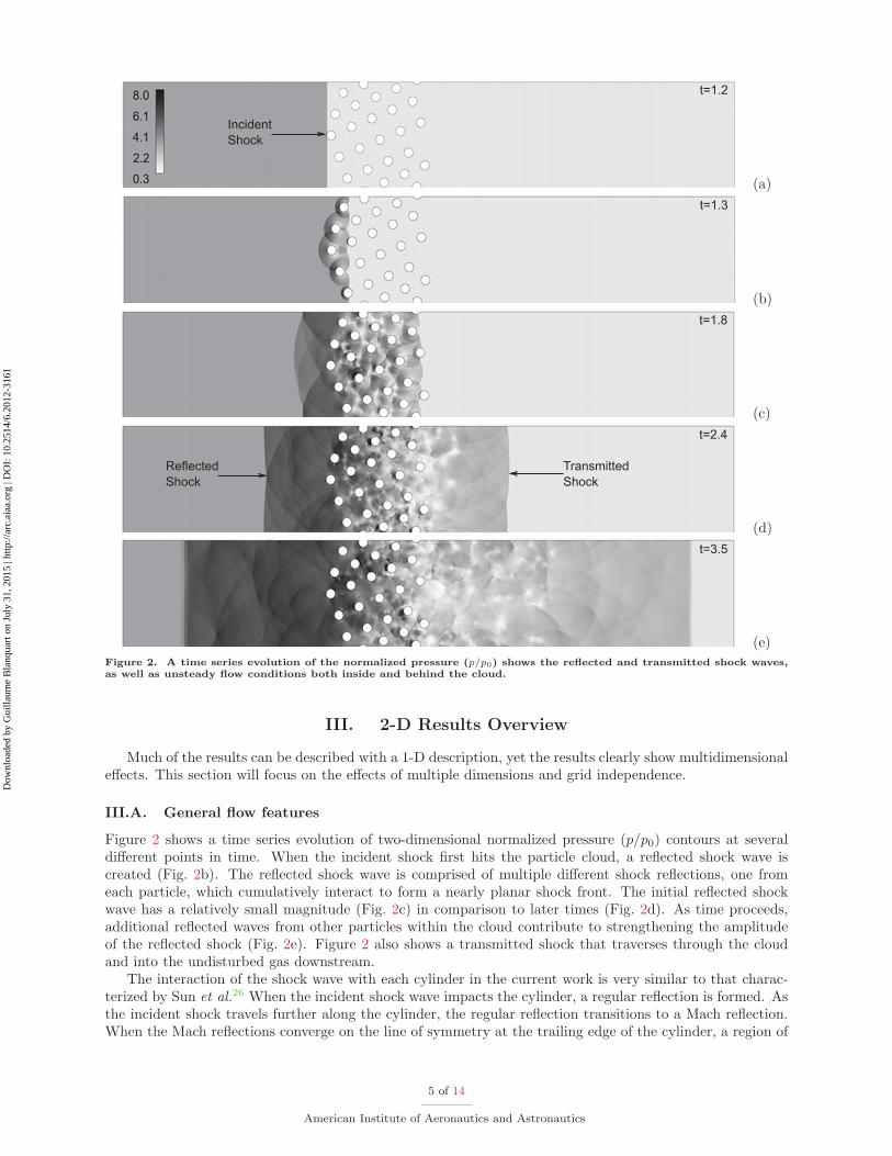
Figure 2. A time series evolution of the normalized pressure (p/p0) shows the reflected and transmitted shock waves,as well as unsteady flow conditions both inside and behind the cloud.

III. 2-D Results Overview

Much of the results can be described with a 1-D description, yet the results clearly show multidimensionaleffects. This section will focus on the effects of multiple dimensions and grid independence.

III.A. General flow features

Figure 2 shows a time series evolution of two-dimensional normalized pressure (p/p0) contours at severaldifferent points in time. When the incident shock first hits the particle cloud, a reflected shock wave iscreated (Fig. 2b). The reflected shock wave is comprised of multiple different shock reflections, one fromeach particle, which cumulatively interact to form a nearly planar shock front. The initial reflected shockwave has a relatively small magnitude (Fig. 2c) in comparison to later times (Fig. 2d). As time proceeds,additional reflected waves from other particles within the cloud contribute to strengthening the amplitudeof the reflected shock (Fig. 2e). Figure 2 also shows a transmitted shock that traverses through the cloudand into the undisturbed gas downstream.

The interaction of the shock wave with each cylinder in the current work is very similar to that charac-terized by Sun et al.26 When the incident shock wave impacts the cylinder, a regular reflection is formed. Asthe incident shock travels further along the cylinder, the regular reflection transitions to a Mach reflection.When the Mach reflections converge on the line of symmetry at the trailing edge of the cylinder, a region of

5 of 14

American Institute of Aeronautics and Astronautics

Dow

nloa

ded

by G

uilla

ume

Bla

nqua

rt o

n Ju

ly 3

1, 2

015

| http

://ar

c.ai

aa.o

rg |

DO

I: 1

0.25

14/6

.201

2-31

61

−2.5 −1.5 −0.5 0.5 1.5 2.5 3.50

1

2

3

4

5

6

Pre

ssur

e p/

p 0

x

132652105

Points / Particle

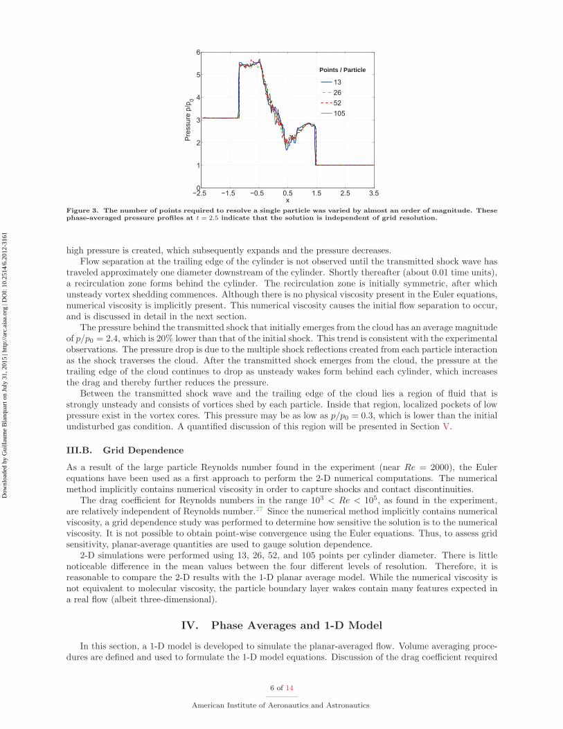
Figure 3. The number of points required to resolve a single particle was varied by almost an order of magnitude. Thesephase-averaged pressure profiles at t = 2.5 indicate that the solution is independent of grid resolution.

high pressure is created, which subsequently expands and the pressure decreases.Flow separation at the trailing edge of the cylinder is not observed until the transmitted shock wave has

traveled approximately one diameter downstream of the cylinder. Shortly thereafter (about 0.01 time units),a recirculation zone forms behind the cylinder. The recirculation zone is initially symmetric, after whichunsteady vortex shedding commences. Although there is no physical viscosity present in the Euler equations,numerical viscosity is implicitly present. This numerical viscosity causes the initial flow separation to occur,and is discussed in detail in the next section.

The pressure behind the transmitted shock that initially emerges from the cloud has an average magnitudeof p/p0 = 2.4, which is 20% lower than that of the initial shock. This trend is consistent with the experimentalobservations. The pressure drop is due to the multiple shock reflections created from each particle interactionas the shock traverses the cloud. After the transmitted shock emerges from the cloud, the pressure at thetrailing edge of the cloud continues to drop as unsteady wakes form behind each cylinder, which increasesthe drag and thereby further reduces the pressure.

Between the transmitted shock wave and the trailing edge of the cloud lies a region of fluid that isstrongly unsteady and consists of vortices shed by each particle. Inside that region, localized pockets of lowpressure exist in the vortex cores. This pressure may be as low as p/p0 = 0.3, which is lower than the initialundisturbed gas condition. A quantified discussion of this region will be presented in Section V.

III.B. Grid Dependence

As a result of the large particle Reynolds number found in the experiment (near Re = 2000), the Eulerequations have been used as a first approach to perform the 2-D numerical computations. The numericalmethod implicitly contains numerical viscosity in order to capture shocks and contact discontinuities.

The drag coefficient for Reynolds numbers in the range 103 < Re < 105, as found in the experiment,are relatively independent of Reynolds number.27 Since the numerical method implicitly contains numericalviscosity, a grid dependence study was performed to determine how sensitive the solution is to the numericalviscosity. It is not possible to obtain point-wise convergence using the Euler equations. Thus, to assess gridsensitivity, planar-average quantities are used to gauge solution dependence.

2-D simulations were performed using 13, 26, 52, and 105 points per cylinder diameter. There is littlenoticeable difference in the mean values between the four different levels of resolution. Therefore, it isreasonable to compare the 2-D results with the 1-D planar average model. While the numerical viscosity isnot equivalent to molecular viscosity, the particle boundary layer wakes contain many features expected ina real flow (albeit three-dimensional).

IV. Phase Averages and 1-D Model

In this section, a 1-D model is developed to simulate the planar-averaged flow. Volume averaging proce-dures are defined and used to formulate the 1-D model equations. Discussion of the drag coefficient required

6 of 14

American Institute of Aeronautics and Astronautics

Dow

nloa

ded

by G

uilla

ume

Bla

nqua

rt o

n Ju

ly 3

1, 2

015

| http

://ar

c.ai

aa.o

rg |

DO

I: 1

0.25

14/6

.201

2-31

61

to close the 1-D model is provided.

IV.A. Definition of Averages

First, the volume average definitions must be made. The volume average is defined

φ =1

V

∫V

φdV , (5)

where V is the sampling volume including both the continuous and disperse phases. If the volume integralis limited to the continuous phase, the phase average (or Reynolds average) is defined

〈φ〉 = 1

Vc

∫Vc

φdV , (6)

where Vc is the volume inside V that only includes the continuous phase, so that the Reynolds and volumeaverages are related by

φ = αc〈φ〉 . (7)

Finally, the mass average, or Favre average is defined as

φ =ρφ

ρ=

〈ρφ〉〈ρ〉 . (8)

Volume-averages in the transverse direction over the continuous phase are used to obtain one-dimensionalplanar averaged quantities from the two-dimensional solutions for comparison with the 1-D model. Thephase-averaged quantity 〈B〉(x) for a quantity B(x, y) is obtained using Eq. 6, where Vc is a samplingvolume that is thin in the x-direction and spans the entire domain height in the y-direction. This equation isused to determine the phase-averaged quantities for the conserved variables ρ, ρui, and ρeT at each x-positionon the numerical grid. The primitive variables ui and p are determined from these quantities.

IV.B. One-dimensional Equations

The one-dimensional volume-averaged model in this work is based upon the averaging procedures for two-phase gas-particle flows presented in Crowe et al.1 The Navier-Stokes equations form the foundation of themodel. Due to the short timescales under consideration, the interphase mass and heat transfer are considerednegligible. The main effects of viscous stresses are neglected except through their impact on the drag law.

As for the 2-D simulations, the particles are frozen in place, such that the particle velocity is zero andthe volume fraction is only a function of position α = α(x). Momentum coupling between the two phasesis assumed to have dominant contributions from the undisturbed flow force1 and the steady-state drag law.With these assumptions, the one-dimensional, continuous phase, volume-averaged conservation equationsare

∂

∂t(αc〈ρc〉) + ∂

∂x(αc〈ρ〉u) = 0 (9a)

∂

∂t(αc〈ρc〉u) + ∂

∂x

(αc〈ρc〉u2 + 〈p〉) = αd

∂〈p〉∂x

(9b)

− αd

2

Ap

VpCD〈ρc〉|u|u

∂

∂t(αc〈ρc〉eT ) + ∂

∂x

(αc〈ρc〉uhT

)= 0 , (9c)

where the unclosed fluctuation terms are neglected. The total energy and enthalpy are defined by

〈ρ〉eT = 〈ρc〉e+ 1

2〈ρc〉u2 , (10)

〈ρc〉hT = 〈ρc〉e+ 1

2〈ρc〉u2 + 〈p〉 , (11)

7 of 14

American Institute of Aeronautics and Astronautics

Dow

nloa

ded

by G

uilla

ume

Bla

nqua

rt o

n Ju

ly 3

1, 2

015

| http

://ar

c.ai

aa.o

rg |

DO

I: 1

0.25

14/6

.201

2-31

61

−2.5 −1.5 −0.5 0.5 1.5 2.5 3.51

1.5

2

2.5

3

3.5

Den

sity

ρ/ρ 0

x

2−D1−D

(a) Density

−2.5 −1.5 −0.5 0.5 1.5 2.5 3.50

0.2

0.4

0.6

0.8

1

1.2

1.4

Vel

ocity

u

x

2−D1−D

(b) Velocity

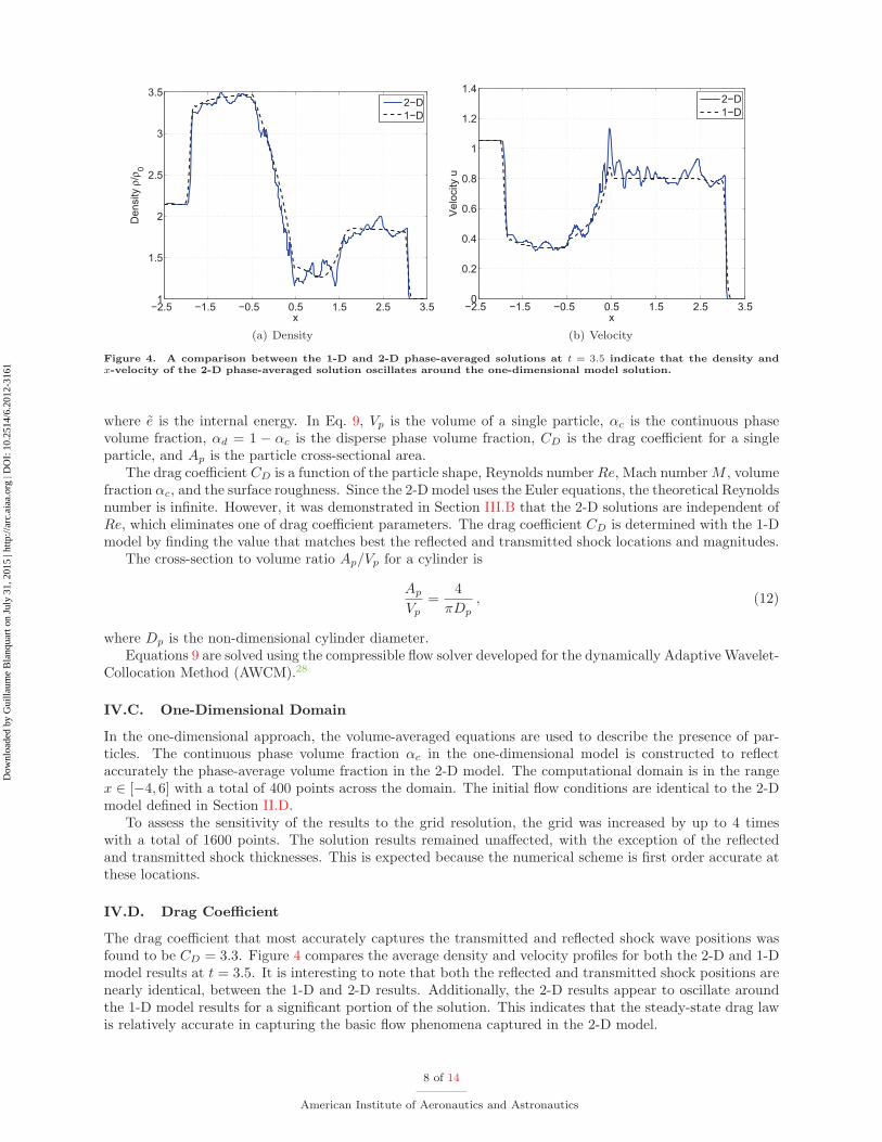
Figure 4. A comparison between the 1-D and 2-D phase-averaged solutions at t = 3.5 indicate that the density andx-velocity of the 2-D phase-averaged solution oscillates around the one-dimensional model solution.

where e is the internal energy. In Eq. 9, Vp is the volume of a single particle, αc is the continuous phasevolume fraction, αd = 1 − αc is the disperse phase volume fraction, CD is the drag coefficient for a singleparticle, and Ap is the particle cross-sectional area.

The drag coefficient CD is a function of the particle shape, Reynolds number Re, Mach numberM , volumefraction αc, and the surface roughness. Since the 2-D model uses the Euler equations, the theoretical Reynoldsnumber is infinite. However, it was demonstrated in Section III.B that the 2-D solutions are independent ofRe, which eliminates one of drag coefficient parameters. The drag coefficient CD is determined with the 1-Dmodel by finding the value that matches best the reflected and transmitted shock locations and magnitudes.

The cross-section to volume ratio Ap/Vp for a cylinder is

Ap

Vp=

4

πDp, (12)

where Dp is the non-dimensional cylinder diameter.Equations 9 are solved using the compressible flow solver developed for the dynamically Adaptive Wavelet-

Collocation Method (AWCM).28

IV.C. One-Dimensional Domain

In the one-dimensional approach, the volume-averaged equations are used to describe the presence of par-ticles. The continuous phase volume fraction αc in the one-dimensional model is constructed to reflectaccurately the phase-average volume fraction in the 2-D model. The computational domain is in the rangex ∈ [−4, 6] with a total of 400 points across the domain. The initial flow conditions are identical to the 2-Dmodel defined in Section II.D.

To assess the sensitivity of the results to the grid resolution, the grid was increased by up to 4 timeswith a total of 1600 points. The solution results remained unaffected, with the exception of the reflectedand transmitted shock thicknesses. This is expected because the numerical scheme is first order accurate atthese locations.

IV.D. Drag Coefficient

The drag coefficient that most accurately captures the transmitted and reflected shock wave positions wasfound to be CD = 3.3. Figure 4 compares the average density and velocity profiles for both the 2-D and 1-Dmodel results at t = 3.5. It is interesting to note that both the reflected and transmitted shock positions arenearly identical, between the 1-D and 2-D results. Additionally, the 2-D results appear to oscillate aroundthe 1-D model results for a significant portion of the solution. This indicates that the steady-state drag lawis relatively accurate in capturing the basic flow phenomena captured in the 2-D model.

8 of 14

American Institute of Aeronautics and Astronautics

Dow

nloa

ded

by G

uilla

ume

Bla

nqua

rt o

n Ju

ly 3

1, 2

015

| http

://ar

c.ai

aa.o

rg |

DO

I: 1

0.25

14/6

.201

2-31

61

Figure 5. An x-t diagram demonstrates the one-dimensional behavior observed in both the one- and two-dimensionalmodel results. Six different regions are identified, which include the (0) undisturbed gas, (1) fluid behind the transmittedshock ST , (2) fluid between the contact C and the cloud’s trailing edge, (3) expansion across the cloud, (4) fluid behindthe reflected shock, and (5) incident shock condition.

The drag coefficient CD = 3.3 is a factor of 2.8 higher than the expected single cylinder value CD ≈ 1.2for an incompressible flow at Re = 2000. This increase in drag coefficient has two main origins: the closepacking of particles and compressibility effects.

In incompressible dense particle clouds, the drag coefficient on a single particle is increased due to theclose proximity of neighboring particles. As discussed earlier, numerous different models have been proposedthat modify the drag coefficient to account for a large disperse phase volume fraction.4,5, 7, 29 Each of thesemodels involve a correction to the drag coefficient or friction factor in such a way that the drag force in aparticle cloud can be expressed as FD = g(αc)FD0

, where FD0is the drag force using the standard drag

coefficient, and g(αc) is a correction function (voidage function7).In addition to close particle proximity, the drag in the current model is anticipated to depend on the flow

Mach number as well. Ideally, one could formulate a correlation of the form

FD = g(αc)h(M)FD0 , (13)

where the particle proximity and Mach number effects are independent. However, the presence of transonicflow conditions and unsteady compression wave generation from the cloud suggests that the effects of thesetwo parameters are likely to be highly linked in the present 2-D simulations.

If Eq. 13 were assumed to be true and that g(αc) for spheres resembles g(αc) for cylinders, the increase indrag coefficient can be estimated. The model of di Felice7 predicts g(αc) = 1.8 for Re = 2000 and αc = 0.85.The average Mach number across the cloud is M ≈ 0.4. With this Mach number, the drag coefficient isexpected to increase by a factor of 1.1.27 If this were the case, the product of g(αc) = 1.8 and h(M) = 1.1gives an increase of 2.0 (instead of 2.8), which is roughly 30% less.

V. Comparison of 1-D and 2-D Models

V.A. General Flow Description

The general behavior of the shock interaction with the particle cloud is best described using an x-t diagram.Figure 5 shows a typical x-t diagram that is specific to the early interactions where the particles can beassumed to be frozen in place. Similar x-t diagrams can be found in Rogue et al.6 and Miura and Glass.10

Figure 5 shows six different fluid regions, which include the (0) undisturbed gas, (1) fluid behind the trans-mitted shock ST , (2) fluid between the contact C and the cloud’s trailing edge, (3) the expansion across thecloud, (4) the fluid behind the reflected shock SR, and (5) flow conditions upstream of the initial shock SI .

When the original shock impacts the leading edge of the cloud, a portion of it is transmitted (ST ) and partof it is reflected (SR). An expansion fan moves through the cloud behind the transmitted shock ST , whichstarts the formation of the pressure gradient across the cloud. When the transmitted shock emerges from thecloud’s trailing edge, a contact discontinuity C and a rarefaction wave R are created. The contact propagatesdownstream and separates region 1 and 2. The rarefaction wave stops the expansion fan’s propagation and

9 of 14

American Institute of Aeronautics and Astronautics

Dow

nloa

ded

by G

uilla

ume

Bla

nqua

rt o

n Ju

ly 3

1, 2

015

| http

://ar

c.ai

aa.o

rg |

DO

I: 1

0.25

14/6

.201

2-31

61

(a) One-dimensional density (b) Two-dimensional density

Figure 6. x-t diagrams for density compare the (a) one-dimensional and (b) two-dimensional planar average solutions.

sets up a steady-state pressure gradient across the cloud (region 3). Additionally, when the rarefactionreaches the leading edge of the cloud, the pressure in region 4, which was gradually increasing from thecumulative addition of compression waves CW, becomes constant.

The steady-state pressure gradient will not form immediately after the rarefaction R passes back throughthe cloud. Instead, the pressure inside the cloud will fluctuate about its mean value, emitting acoustic wavesaway from the cloud. These fluctuations are shown in Fig. 5 as dashed lines propagating away from thecloud (labeled CW) along the characteristic lines u− c and u+ c.

V.B. Model Similarities

As mentioned earlier, one-dimensional quantities can be obtained from the 2-D data by taking the phase-average defined in Eq. 6. The 2-D solution used for comparison is the case where 52 grid cells are usedper cylinder diameter. The sampling volume spans Dp/2 in the x-direction and the entire domain in they-direction. In order to prevent shock widening from the volume averaging process, sampling volumes of asingle grid cell in the x-direction are used in regions where the reflected and transmitted shocks are located.

Figures 6, 7, and 8 compare x-t diagrams for the density, velocity, and pressure, respectively. Both the1-D and 2-D models show the basic flow behavior described in the x-t diagram (5) of the previous section.In the density diagram (Fig. 6), both models show the reflected (SR) and transmitted (ST ) shocks when theincident shock SI first impacts the particle cloud. The expansion across the cloud is captured both duringits formation and after it has formed a steady-state expansion. The existence of the contact discontinuity Cis consistent between both models, and the density magnitude and slope are similar as well.

The velocity in Fig. 7 is similar between both models. Although the velocity contour shows some un-steadiness primarily behind the cloud, Fig. 4(b) indicates that at t = 3.5 the 2-D solution oscillates aboutthe 1-D solution velocity.

V.C. Model Differences

There is a noticeable difference in behavior during the initial transient period (1.2 < t < 1.8) from whenthe shock wave first enters the cloud until it leaves. The transmitted density is higher in the 2-D model(Fig. 6(b)) than it is in the 1-D model (Fig. 6(a)). This is attributed to the fact that as the shock first passesthrough the cloud, the flow around the cylinders has not detached yet to form a wake. The drag coefficientin the steady-state model assumes a fully developed and separated wake, which causes the 1-D model tooverestimate the particle drag during the initial shock propagation.

Figure 7 shows that the shock traverses the cloud with a higher speed in the 2-D model than it does inthe 1-D model. For each point in space inside the cloud just after the shock has passed, the velocity remainshigh for t ≈ 0.2 and then the mean velocity drops rapidly. The rapid drop in velocity is characterized by

10 of 14

American Institute of Aeronautics and Astronautics

Dow

nloa

ded

by G

uilla

ume

Bla

nqua

rt o

n Ju

ly 3

1, 2

015

| http

://ar

c.ai

aa.o

rg |

DO

I: 1

0.25

14/6

.201

2-31

61

(a) One-dimensional velocity (b) Two-dimensional velocity

Figure 7. x-t diagrams for velocity compare the (a) one-dimensional and (b) two-dimensional planar average solutions.

the onset of flow separation and wake formation. In the 1-D model, the velocity experiences a more gradualdecay and this dynamic process is not captured.

In Fig. 8, the 2-D x-t diagram shows the presence of coherent compression waves propagating in both the−x and +x-directions away from the cloud region. These waves are absent in the 1-D model. Inside the cloudof the 2-D model, it is difficult to trace the characteristic lines, which suggests that the compression wavesoriginate from the cloud itself. This is consistent with the observation of coherent localized compression wavesin the 2-D pressure contour plot in Fig. 2. These waves appear to be repeated internal reflection/transmissionwaves created by the initial shock that continue to reverberate inside the cloud.

Pressure is normally constant across a true contact discontinuity. In the 1-D model, this is shown to betrue (see Fig. 8(a)). In the 2-D model, the contact separates a region of predominantly steady flow (onlydisturbed by weak periodic acoustic waves), and a region of unsteady flow with large oscillating pressuredisturbances associated with vortex shedding.

Figure 9 compares the pressure at t = 3.5 for the 1-D and 2-D models. The average pressure between thecloud trailing edge at x = 0.5 and the contact discontinuity at x = 1.5 is consistently lower than that predictedby the 1-D model. In its current form, the 1-D model is incapable of reproducing this unsteady behavior.Since the unsteady flow features travel downstream at the mean fluid velocity, the contact discontinuitymarks the transition between a smooth transmitted shock region and an unsteady wake region.

The equations solved in the 1-D model do not include the unclosed fluctuation terms created during thevolume-averaging procedure.1 This is a reasonable assumption in dilute multiphase flows, such as dustygases.9,10,11,12,30 However, in dense flows this assumption may not be appropriate. The volume-averagedmomentum equation (Eq. 9b) contains one unclosed Reynolds stress term.1,31 It is convenient to define atotal pressure pT to be the sum of the volume-averaged pressure 〈p〉 and the Reynolds stress

pT = 〈p〉+ αc〈ρcu′′u′′〉 . (14)

This is the 1-D equivalent formulation of the multidimensional pressure tensor.1,31

Figure 9 shows the 1-D and 2-D pressures 〈p〉, as well as the the total pressure pT . The addition ofthe unclosed fluctuation Reynolds stress term accounts for the difference between the solutions. The 2-D〈p〉 and pT quantities are identical outside of the cloud and the unsteady fluctuation region, but only thetotal pressure matches accurately the 1-D model solution inside the cloud and unsteady region. In order tomodel these interactions accurately using a 1-D model, models must be created that capture these unsteadyeffects.

11 of 14

American Institute of Aeronautics and Astronautics

Dow

nloa

ded

by G

uilla

ume

Bla

nqua

rt o

n Ju

ly 3

1, 2

015

| http

://ar

c.ai

aa.o

rg |

DO

I: 1

0.25

14/6

.201

2-31

61

(a) One-dimensional pressure (b) Two-dimensional pressure

Figure 8. x-t diagrams for pressure compare the (a) one-dimensional and (b) two-dimensional planar average solutions.The contact discontinuity at x = 1.5 marks the interface between steady and unsteady flow regions.

−2.5 −1.5 −0.5 0.5 1.5 2.5 3.51

2

3

4

5

6

7

Pre

ssur

e p/

p 0

x

1−D2−D2−D+αc<ρu"u">

Figure 9. At t = 3.5, the 2-D planar averaged solution is lower than the 1-D model between the cloud’s trailing edgeand the contact discontinuity.

VI. Discussion

It is difficult to make a direct comparison of the current 2-D work with that observed experimentally inRef. 20 for two primary reasons: 1) because of the difference in dimensionality (2-D vs. 3-D), and 2) thetimescales of interest in the experiment are over several hundred microseconds, whereas the timescales ofinterest in this work are only over the first 30μs. However, further insight into the fine details of the flowbehavior can still be made.

In the experiment,20 the momentum and energy fluxes downstream of the cloud are reduced by 30-40%,which is a substantially larger decrease than that observed in dusty gases.10 The momentum and energyflux changes predicted in the current work show a similar large reduction (about 45%). This larger value isexpected because of the higher particle drag on cylinders compared to spheres.

In Ref. 20, the Schlieren images show transmitted and reflected shock waves. Behind the transmittedshock is a region of relatively constant density fluid. Between the transmitted shock and the trailing edgeof the cloud, there is a region of darkness closer to the cloud’s trailing edge and a light colored region closerto the transmitted shock. Based upon the current analysis, it seems that this transition from light to darkmay actually be the contact discontinuity, where the light color in the Schlieren image depicts the drop indensity across the contact. The presence of this contact is consistent with that in Ref. 10. The unsteady

12 of 14

American Institute of Aeronautics and Astronautics

Dow

nloa

ded

by G

uilla

ume

Bla

nqua

rt o

n Ju

ly 3

1, 2

015

| http

://ar

c.ai

aa.o

rg |

DO

I: 1

0.25

14/6

.201

2-31

61

region between the contact and the cloud’s trailing edge may appear dark in the Schlieren images20 becausethe image is created with a plane-averaged line of sight.

From this perspective, the 2-D model seems to capture the essential flow physics. The transmitted andreflected shock waves regain a planar shape after emerging from the cloud. A contact discontinuity is formedat the trailing edge of the cloud and marks the interface between the laminar fluid in region 1 and anunsteady region 2. The flow in region 2 may be turbulent, but this cannot be confirmed without performingthree-dimensional computations.

VII. Conclusions

One- and two-dimensional simulations have been performed to study the early stages after a shock waveimpinges normally upon a planar cloud of particles. Two-dimensional simulations are performed using afinite number of particles, which are modeled as cylinders frozen in space. Planar phase-averages are usedto create equivalent one-dimensional profiles.

The x-t diagrams show reflected and transmitted shock waves. An expansion fan propagates into thecloud and is stabilized in place by the passage of a rarefaction wave that is created after the transmittedshock emerges from the cloud. This creates a steady-state expansion across the particle cloud that acceleratesthe flow. Finally, a contact discontinuity is formed at the cloud’s trailing edge when the transmitted shockemerges from the cloud.

The 2-D simulation results exhibit strong unsteady effects. Shock reflections from a finite number ofdiscrete particles create a noisy source of compression waves inside the particle cloud, long after the shockwave has left the cloud. Localized regions of transonic Mach numbers near the trailing edge of the cloudcontribute to this source of compression waves. Additionally, the unsteady flow behind the cloud is char-acterized by vortical structures that propagate downstream. The contact discontinuity marks the interfacebetween the unsteady flow region behind the particle cloud and the higher density fluid located just behindthe transmitted shock. Similar flow features have been observed in the experimental work in Ref. 20.

An equivalent one-dimensional model problem is created using volume-averaged equations. The 1-Dmodel neglects all unclosed fluctuation terms, such as the Reynolds stress term, and models the particledrag with the steady-state drag law and the undisturbed flow force. A drag coefficient is obtained thatprovides a match of the reflected and transmitted shock wave’s locations and magnitudes. The 1-D modelcaptures the one-dimensional flow behavior well, including the reflected and transmitted shock waves, thecontact discontinuity, and the expansion across the cloud.

The 1-D model does not capture unsteady effects such as a time lag in the drag coefficient due to adelay in boundary layer separation, compression wave generation from localized regions where transonicflow conditions exist, and energy contained in unclosed fluctuation terms such as the Reynolds stress andturbulent kinetic energy. While it may be satisfactory to neglect these unclosed fluctuation terms in diluteflows, these terms play a dominant role in dense flows and must be modeled.

Acknowledgments

The authors would like to thank Karen Oren for her contribution to this work.

References

1Crowe, C. T., Schwarzkopf, J. D., Sommerfeld, M., and Tsuji, Y., Multiphase Flows with Droplets and Particles, CRCPress, 2nd ed., 2012.

2Zhang, F., Frost, D. L., Thibault, P. A., and Murray, S. B., “Explosive Dispersal of Solid Particles,” Shock Waves,Vol. 10, 2001, pp. 431–443.

3Igra, O. and Ben-Dor, G., “Dusty Shock Waves,” Applied Mechanics, Vol. 41, 1988, pp. 379–437.4Ergun, S., “Fluid flow through packed columns,” Chem. Engr. Prog., Vol. 48, 1952, pp. 89.5Gibilaro, L. G., Di Felice, R., Waldram, S. P., and Foscolo, P. U., “Generalized Friction Factor and Drag Coefficient

Correlations for Fluid-Particle Interactions,” Chemical Engineering Science, Vol. 40, No. 10, 1985, pp. 1817–1823.6Rogue, X., Rodriguez, G., Haas, J., and Saurel, R., “Experimental and numerical investigation of the shock-induced

fluidization of a particles bed,” Shock Waves, Vol. 8, No. 1, Feb. 1998, pp. 29–45.7Di Felice, R., “The Voidage Function for Fluid-Particle Interaction Systems,” Int. J. Multiphase Flow , Vol. 20, 1994,

pp. 153–159.8Carrier, G., “Shock waves in a dusty gas,” J. Fluid Mech., , No. March, 1958.

13 of 14

American Institute of Aeronautics and Astronautics

Dow

nloa

ded

by G

uilla

ume

Bla

nqua

rt o

n Ju

ly 3

1, 2

015

| http

://ar

c.ai

aa.o

rg |

DO

I: 1

0.25

14/6

.201

2-31

61

9Miura, H. and Glass, I. I., “On a Dusty-Gas Shock Tube,” Proceedings of the Royal Society A: Mathematical, Physicaland Engineering Sciences, Vol. 382, No. 1783, Aug. 1982, pp. 373–388.

10Miura, H. and Glass, I. I., “On the Passage of a Shock Wave Through a Dusty-Gas Layer,” Proceedings of the RoyalSociety A: Mathematical, Physical and Engineering Sciences, Vol. 385, No. 1788, Jan. 1983, pp. 85–105.

11Miura, H., “Decay of shock waves in a dusty-gas shock tube,” Fluid Dynamics Research, Vol. 6, No. 5-6, Dec. 1990,pp. 251–259.

12Saito, T., “Numerical Analysis of Dusty-Gas Flows,” J Comp Phys, Vol. 176, No. 1, 2002, pp. 129–144.13Baer, M. R. and Nunziato, J. W., “A Two-Phase Mixture Theory for the Deflagration-to-Detonation Transition (DDT)

in Reactive Granular Materials,” Int. J. Multiphase Flow , Vol. 12, No. 6, 1986, pp. 861–889.14Powers, J. M., Stewart, D. S., and Krier, H., “Theory of Two-Phase Detonation-Part I: Modeling,” Combustion and

Flame, Vol. 80, No. 3-4, 1990, pp. 264–279.15Baer, M. R., “Shock Wave Structure in Heterogeneous Reactive Media,” 21st Int. Symp. Shock Waves, 1997, pp. 923–927.16Anderson, M. U., Graham, R. a., and Holman, G. T., “Time-resolved shock compression of porous rutile: Wave dispersion

in porous solids,” AIP Conference Proceedings, Vol. 309, No. 1994, 1994, pp. 1111–1114.17Sommerfeld, M., “The unsteadiness of shock waves propagating through gas-particle mixtures,” Experiments in Fluids,

Vol. 3, No. 4, 1985, pp. 197–206.18Boiko, V., Kiselev, V., Kiselev, S., a.N. Papyrin, Poplavsky, S., and Fomin, V., “Shock wave interaction with a cloud of

particles,” Shock Waves, Vol. 7, No. 5, Oct. 1997, pp. 275–285.19Wagner, J. L., Beresh, S. J., Kearney, S. P., Trott, W. M., Castaneda, J. N., Pruett, B. O. M., and Baer, M. R.,

“Interaction of a Planar Shock with a Dense Field of Particles in a Multiphase Shock Tube,” Proc. 49th AIAA AerospaceSciences Meeting, Vol. 188, 2011, pp. 1–13.

20Wagner, J. L., Beresh, S. J., Kearney, S. P., Trott, W. M., Castaneda, J. N., Pruett, B. O., and Baer, M. R., “Amultiphase shock tube for shock wave interactions with dense particle fields,” Experiments in Fluids, Vol. (in press), Feb. 2012.

21Boiko, V. M. and Poplavski, S. V., “On the Dynamics of Drop Acceleration at the Early Stage of Velocity Relaxation ina Shock Wave,” Comb. Exp. Shock Waves, Vol. 45, No. 2, 2009, pp. 198–204.

22Clemins, A., “Representation of two-phase flows by volume averaging,” International Journal of Multiphase Flow , Vol. 14,No. 1, Jan. 1988, pp. 81–90.

23Roe, P. L. and Pike, J., “Efficient construction and utilisation of approximate Riemann solutions,” Computing methodsin applied sciences and engineering, VI , 1984, pp. 499–518.

24Toro, E. F., Riemann Solvers and Numerical Methods for Fluid Dynamics, Spring, 2nd ed., 1999.25van Leer, B., “Towards the ultimate conservative difference scheme. V. A second-order sequel to Godunov’s method,”

Journal of Computational Physics, Vol. 32, No. 1, 1979, pp. 101–136.26Sun, M., Saito, T., Takayama, K., and Tanno, H., “Unsteady drag on a sphere by shock wave loading,” Shock Waves,

Vol. 14, No. 1-2, June 2005, pp. 3–9.27White, F. M., Fluid Mechanics, McGraw Hill, New York, seventh ed., 2011.28Regele, J. D. and Vasilyev, O. V., “An adaptive wavelet-collocation method for shock computations,” International

Journal of Computational Fluid Dynamics, Vol. 23, No. 7, Aug. 2009, pp. 503–518.29Makkawi, Y., “The voidage function and effective drag force for fluidized beds,” Chemical Engineering Science, Vol. 58,

No. 10, May 2003, pp. 2035–2051.30Saito, T., Saba, M., Sun, M., and Takayama, K., “The effect of an unsteady drag force on the structure of a non-

equilibrium region behind a shock wave in a gas-particle mixture,” Shock Waves, Vol. 17, No. 4, Oct. 2007, pp. 255–262.31Drew, D. A. and Passman, S. L., “Theory of Multicomponent Fluids,” Applied Mathematical Sciences, Vol. 135, 1999.

14 of 14

American Institute of Aeronautics and Astronautics

Dow

nloa

ded

by G

uilla

ume

Bla

nqua

rt o

n Ju

ly 3

1, 2

015

| http

://ar

c.ai

aa.o

rg |

DO

I: 1

0.25

14/6

.201

2-31

61