Introduction to Gaussian Processes

Neil D. Lawrence

GPMC6th February 2017

Book

Rasmussen and Williams (2006)

Outline

The Gaussian Density

Covariance from Basis Functions

Outline

The Gaussian Density

Covariance from Basis Functions

The Gaussian Density

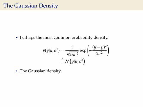
I Perhaps the most common probability density.

p(y|µ, σ2) =1

√

2πσ2exp

(−

(y − µ)2

2σ2

)4= N

(y|µ, σ2

)I The Gaussian density.

Gaussian Density

0

1

2

3

0 1 2

p(h|µ,σ

2 )

h, height/m

The Gaussian PDF with µ = 1.7 and variance σ2 = 0.0225. Meanshown as red line. It could represent the heights of apopulation of students.

Gaussian Density

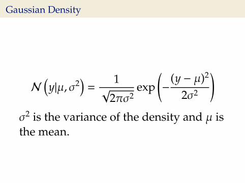
N

(y|µ, σ2

)=

1√

2πσ2exp

(−

(y − µ)2

2σ2

)σ2 is the variance of the density and µ isthe mean.

Two Important Gaussian Properties

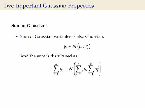
Sum of Gaussians

I Sum of Gaussian variables is also Gaussian.

yi ∼ N(µi, σ

2i

)

And the sum is distributed as

n∑i=1

yi ∼ N

n∑i=1

µi,n∑

i=1

σ2i

(Aside: As sum increases, sum of non-Gaussian, finitevariance variables is also Gaussian [central limit theorem].)

Two Important Gaussian Properties

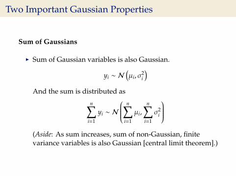
Sum of Gaussians

I Sum of Gaussian variables is also Gaussian.

yi ∼ N(µi, σ

2i

)And the sum is distributed as

n∑i=1

yi ∼ N

n∑i=1

µi,n∑

i=1

σ2i

(Aside: As sum increases, sum of non-Gaussian, finitevariance variables is also Gaussian [central limit theorem].)

Two Important Gaussian Properties

Sum of Gaussians

I Sum of Gaussian variables is also Gaussian.

yi ∼ N(µi, σ

2i

)And the sum is distributed as

n∑i=1

yi ∼ N

n∑i=1

µi,n∑

i=1

σ2i

(Aside: As sum increases, sum of non-Gaussian, finitevariance variables is also Gaussian [central limit theorem].)

Two Important Gaussian Properties

Sum of Gaussians

I Sum of Gaussian variables is also Gaussian.

yi ∼ N(µi, σ

2i

)And the sum is distributed as

n∑i=1

yi ∼ N

n∑i=1

µi,n∑

i=1

σ2i

(Aside: As sum increases, sum of non-Gaussian, finitevariance variables is also Gaussian [central limit theorem].)

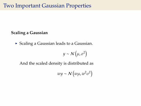
Two Important Gaussian Properties

Scaling a Gaussian

I Scaling a Gaussian leads to a Gaussian.

y ∼ N(µ, σ2

)And the scaled density is distributed as

wy ∼ N(wµ,w2σ2

)

Two Important Gaussian Properties

Scaling a Gaussian

I Scaling a Gaussian leads to a Gaussian.

y ∼ N(µ, σ2

)

And the scaled density is distributed as

wy ∼ N(wµ,w2σ2

)

Two Important Gaussian Properties

Scaling a Gaussian

I Scaling a Gaussian leads to a Gaussian.

y ∼ N(µ, σ2

)And the scaled density is distributed as

wy ∼ N(wµ,w2σ2

)

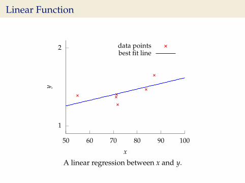
Linear Function

1

2

50 60 70 80 90 100

y

x

data pointsbest fit line

A linear regression between x and y.

Regression Examples

I Predict a real value, yi given some inputs xi.I Predict quality of meat given spectral measurements

(Tecator data).I Radiocarbon dating, the C14 calibration curve: predict age

given quantity of C14 isotope.I Predict quality of different Go or Backgammon moves

given expert rated training data.

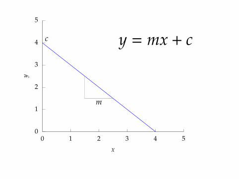
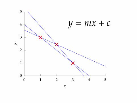
y = mx + c

0

1

2

3

4

5

0 1 2 3 4 5

y

x

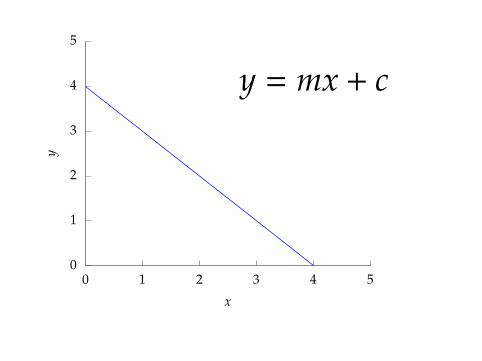
y = mx + c

0

1

2

3

4

5

0 1 2 3 4 5

y

x

y = mx + cc

m

0

1

2

3

4

5

0 1 2 3 4 5

y

x

y = mx + cc

m

0

1

2

3

4

5

0 1 2 3 4 5

y

x

y = mx + cc

m

0

1

2

3

4

5

0 1 2 3 4 5

y

x

y = mx + c

0

1

2

3

4

5

0 1 2 3 4 5

y

x

y = mx + c

0

1

2

3

4

5

0 1 2 3 4 5

y

x

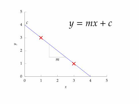
y = mx + c

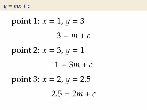
y = mx + c

point 1: x = 1, y = 3

3 = m + c

point 2: x = 3, y = 1

1 = 3m + c

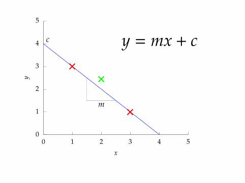
point 3: x = 2, y = 2.5

2.5 = 2m + c

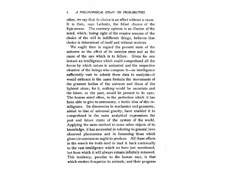
6 A PHILOSOPHICAL ESSAY ON PROBABILITIES.

height: "The day will come when, by study pursued

through several ages, the things now concealed will

appear with evidence; and posterity will be astonished

that truths so clear had escaped us.' '

Clairaut then

undertook to submit to analysis the perturbations which

the comet had experienced by the action of the two

great planets, Jupiter and Saturn; after immense cal-

culations he fixed its next passage at the perihelion

toward the beginning of April, 1759, which was actually

verified by observation. The regularity which astronomyshows us in the movements of the comets doubtless

exists also in all phenomena. -

The curve described by a simple molecule of air or

vapor is regulated in a manner just as certain as the

planetary orbits;the only difference between them is

that which comes from our ignorance.

Probability is relative, in part to this ignorance, in

part to our knowledge. We know that of three or a

greater number of events a single one ought to occur;

but nothing induces us to believe that one of them will

occur rather than the others. In this state of indecision

it is impossible for us to announce their occurrence with

certainty. It is, however, probable that one of these

events, chosen at will, will not occur because we see

several cases equally possible which exclude its occur-

rence, while only a single one favors it.

The theory of chance consists in reducing all the

events of the same kind to a certain number of cases

equally possible, that is to say, to such as we may be

equally undecided about in regard to their existence,and in determining the number of cases favorable to

the event whose probability is sought. The ratio of

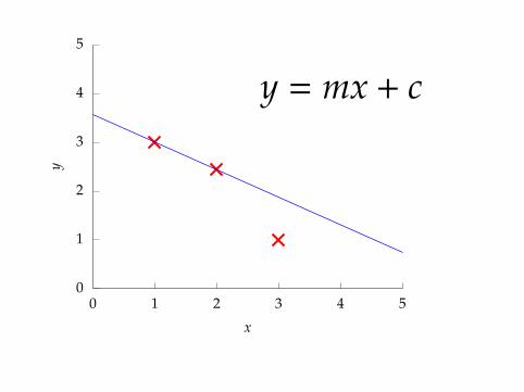
y = mx + c + ε

point 1: x = 1, y = 3

3 = m + c + ε1

point 2: x = 3, y = 1

1 = 3m + c + ε2

point 3: x = 2, y = 2.5

2.5 = 2m + c + ε3

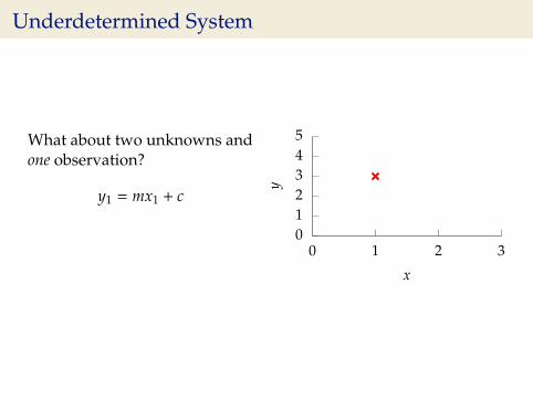
Underdetermined System

What about two unknowns andone observation?

y1 = mx1 + c

012345

0 1 2 3y

x

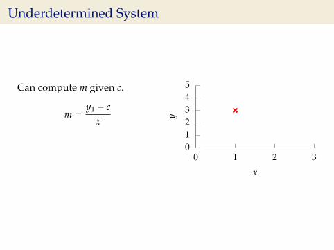
Underdetermined System

Can compute m given c.

m =y1 − c

x

012345

0 1 2 3y

x

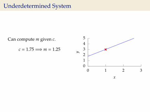
Underdetermined System

Can compute m given c.

c = 1.75 =⇒ m = 1.25

012345

0 1 2 3y

x

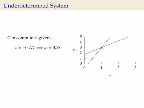
Underdetermined System

Can compute m given c.

c = −0.777 =⇒ m = 3.78

012345

0 1 2 3y

x

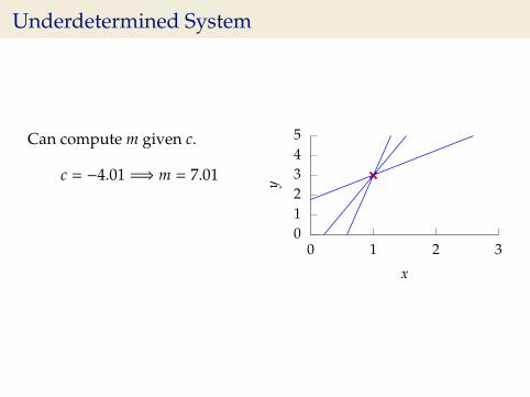
Underdetermined System

Can compute m given c.

c = −4.01 =⇒ m = 7.01

012345

0 1 2 3y

x

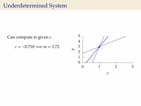
Underdetermined System

Can compute m given c.

c = −0.718 =⇒ m = 3.72

012345

0 1 2 3y

x

Underdetermined System

Can compute m given c.

c = 2.45 =⇒ m = 0.545

012345

0 1 2 3y

x

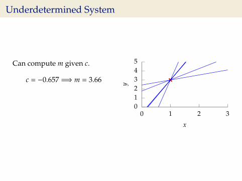
Underdetermined System

Can compute m given c.

c = −0.657 =⇒ m = 3.66

012345

0 1 2 3y

x

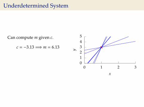
Underdetermined System

Can compute m given c.

c = −3.13 =⇒ m = 6.13

012345

0 1 2 3y

x

Underdetermined System

Can compute m given c.

c = −1.47 =⇒ m = 4.47

012345

0 1 2 3y

x

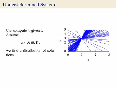
Underdetermined System

Can compute m given c.Assume

c ∼ N (0, 4) ,

we find a distribution of solu-tions.

012345

0 1 2 3y

x

Probability for Under- and Overdetermined

I To deal with overdetermined introduced probabilitydistribution for ‘variable’, εi.

I For underdetermined system introduced probabilitydistribution for ‘parameter’, c.

I This is known as a Bayesian treatment.

Multivariate Prior Distributions

I For general Bayesian inference need multivariate priors.I E.g. for multivariate linear regression:

yi =∑

i

w jxi, j + εi

(where we’ve dropped c for convenience), we need a priorover w.

I This motivates a multivariate Gaussian density.I We will use the multivariate Gaussian to put a prior directly

on the function (a Gaussian process).

Multivariate Prior Distributions

I For general Bayesian inference need multivariate priors.I E.g. for multivariate linear regression:

yi = w>xi,: + εi

(where we’ve dropped c for convenience), we need a priorover w.

I This motivates a multivariate Gaussian density.I We will use the multivariate Gaussian to put a prior directly

on the function (a Gaussian process).

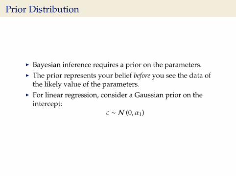
Prior Distribution

I Bayesian inference requires a prior on the parameters.I The prior represents your belief before you see the data of

the likely value of the parameters.I For linear regression, consider a Gaussian prior on the

intercept:c ∼ N (0, α1)

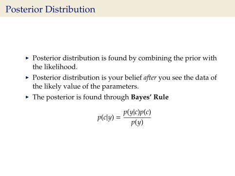
Posterior Distribution

I Posterior distribution is found by combining the prior withthe likelihood.

I Posterior distribution is your belief after you see the data ofthe likely value of the parameters.

I The posterior is found through Bayes’ Rule

p(c|y) =p(y|c)p(c)

p(y)

Bayes Update

0

1

2

-3 -2 -1 0 1 2 3 4c

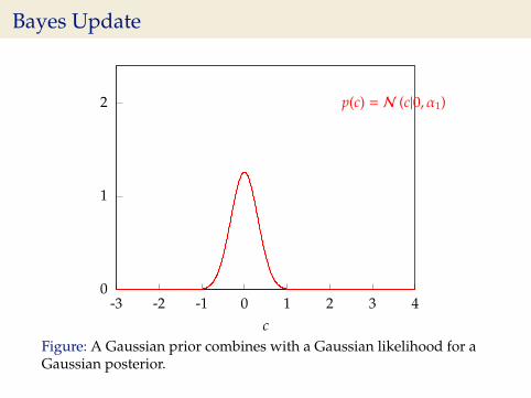
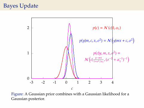
p(c) = N (c|0, α1)

Figure: A Gaussian prior combines with a Gaussian likelihood for aGaussian posterior.

Bayes Update

0

1

2

-3 -2 -1 0 1 2 3 4c

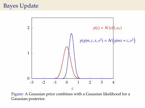
p(c) = N (c|0, α1)

p(y|m, c, x, σ2) = N(y|mx + c, σ2

)

Figure: A Gaussian prior combines with a Gaussian likelihood for aGaussian posterior.

Bayes Update

0

1

2

-3 -2 -1 0 1 2 3 4c

p(c) = N (c|0, α1)

p(y|m, c, x, σ2) = N(y|mx + c, σ2

)p(c|y,m, x, σ2) =

N

(c| y−mx

1+σ2/α1, (σ−2 + α−1

1 )−1)

Figure: A Gaussian prior combines with a Gaussian likelihood for aGaussian posterior.

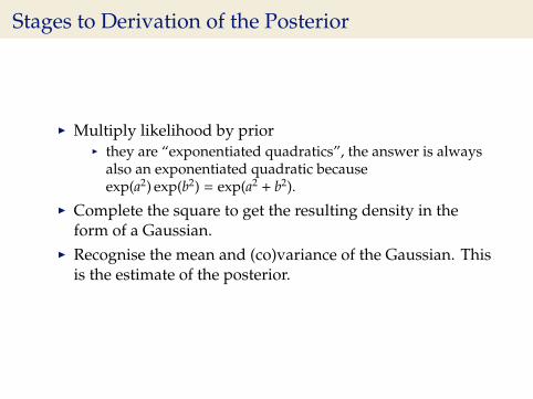
Stages to Derivation of the Posterior

I Multiply likelihood by priorI they are “exponentiated quadratics”, the answer is always

also an exponentiated quadratic becauseexp(a2) exp(b2) = exp(a2 + b2).

I Complete the square to get the resulting density in theform of a Gaussian.

I Recognise the mean and (co)variance of the Gaussian. Thisis the estimate of the posterior.

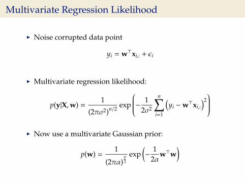
Multivariate Regression Likelihood

I Noise corrupted data point

yi = w>xi,: + εi

I Multivariate regression likelihood:

p(y|X,w) =1

(2πσ2)n/2 exp

− 12σ2

n∑i=1

(yi −w>xi,:

)2

I Now use a multivariate Gaussian prior:

p(w) =1

(2πα)p2

exp(−

12α

w>w)

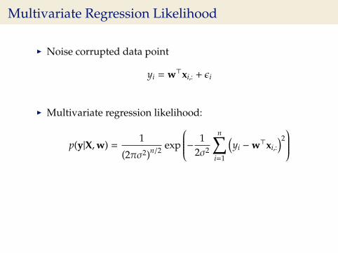
Multivariate Regression Likelihood

I Noise corrupted data point

yi = w>xi,: + εi

I Multivariate regression likelihood:

p(y|X,w) =1

(2πσ2)n/2 exp

− 12σ2

n∑i=1

(yi −w>xi,:

)2

I Now use a multivariate Gaussian prior:

p(w) =1

(2πα)p2

exp(−

12α

w>w)

Multivariate Regression Likelihood

I Noise corrupted data point

yi = w>xi,: + εi

I Multivariate regression likelihood:

p(y|X,w) =1

(2πσ2)n/2 exp

− 12σ2

n∑i=1

(yi −w>xi,:

)2

I Now use a multivariate Gaussian prior:

p(w) =1

(2πα)p2

exp(−

12α

w>w)

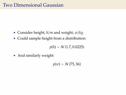
Two Dimensional Gaussian

I Consider height, h/m and weight, w/kg.I Could sample height from a distribution:

p(h) ∼ N (1.7, 0.0225)

I And similarly weight:

p(w) ∼ N (75, 36)

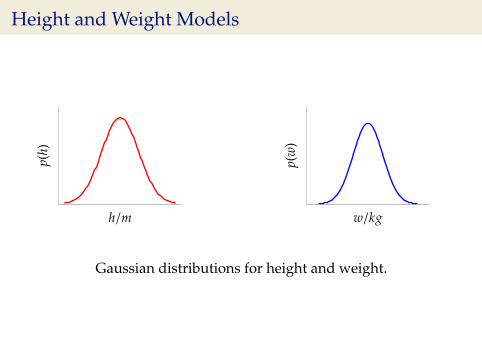
Height and Weight Modelsp(

h)

h/m

p(w

)

w/kg

Gaussian distributions for height and weight.

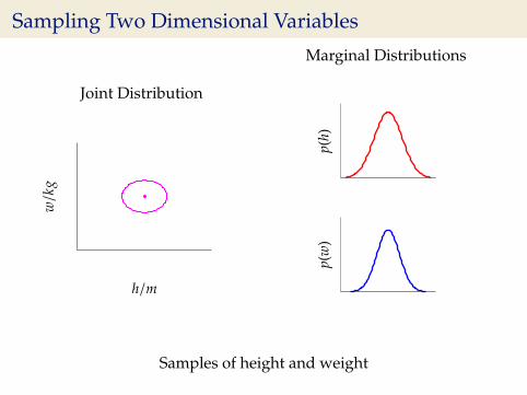
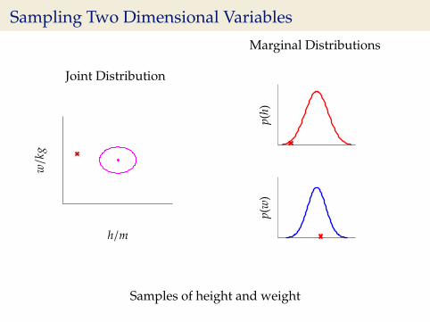
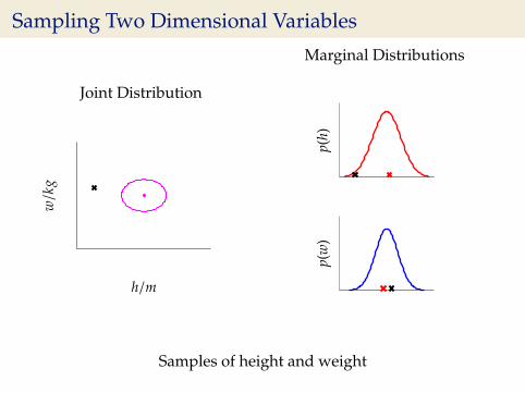
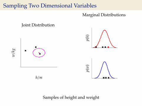
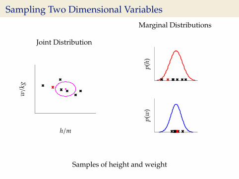
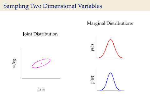
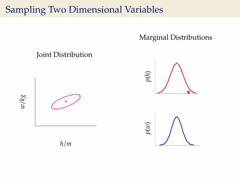
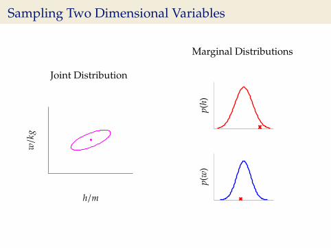
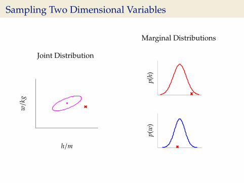
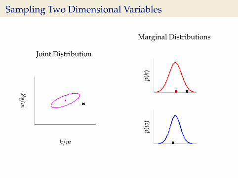
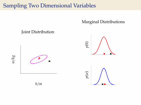
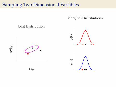
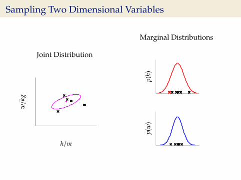
Sampling Two Dimensional Variables

Joint Distribution

w/k

g

h/m

Marginal Distributions

p(h)

p(w

)

Samples of height and weight

Sampling Two Dimensional Variables

Joint Distribution

w/k

g

h/m

Marginal Distributions

p(h)

p(w

)

Samples of height and weight

Sampling Two Dimensional Variables

Joint Distribution

w/k

g

h/m

Marginal Distributions

p(h)

p(w

)

Samples of height and weight

Sampling Two Dimensional Variables

Joint Distribution

w/k

g

h/m

Marginal Distributions

p(h)

p(w

)

Samples of height and weight

Sampling Two Dimensional Variables

Joint Distribution

w/k

g

h/m

Marginal Distributions

p(h)

p(w

)

Samples of height and weight

Sampling Two Dimensional Variables

Joint Distribution

w/k

g

h/m

Marginal Distributions

p(h)

p(w

)

Samples of height and weight

Sampling Two Dimensional Variables

Joint Distribution

w/k

g

h/m

Marginal Distributions

p(h)

p(w

)

Samples of height and weight

Sampling Two Dimensional Variables

Joint Distribution

w/k

g

h/m

Marginal Distributions

p(h)

p(w

)

Samples of height and weight

Sampling Two Dimensional Variables

Joint Distribution

w/k

g

h/m

Marginal Distributions

p(h)

p(w

)

Samples of height and weight

Sampling Two Dimensional Variables

Joint Distribution

w/k

g

h/m

Marginal Distributions

p(h)

p(w

)

Samples of height and weight

Sampling Two Dimensional Variables

Joint Distribution

w/k

g

h/m

Marginal Distributions

p(h)

p(w

)

Samples of height and weight

Sampling Two Dimensional Variables

Joint Distribution

w/k

g

h/m

Marginal Distributions

p(h)

p(w

)

Samples of height and weight

Sampling Two Dimensional Variables

Joint Distribution

w/k

g

h/m

Marginal Distributions

p(h)

p(w

)

Samples of height and weight

Sampling Two Dimensional Variables

Joint Distribution

w/k

g

h/m

Marginal Distributions

p(h)

p(w

)

Samples of height and weight

Sampling Two Dimensional Variables

Joint Distribution

w/k

g

h/m

Marginal Distributions

p(h)

p(w

)

Samples of height and weight

Sampling Two Dimensional Variables

Joint Distribution

w/k

g

h/m

Marginal Distributions

p(h)

p(w

)

Samples of height and weight

Sampling Two Dimensional Variables

Joint Distribution

w/k

g

h/m

Marginal Distributions

p(h)

p(w

)

Samples of height and weight

Sampling Two Dimensional Variables

Joint Distribution

w/k

g

h/m

Marginal Distributions

p(h)

p(w

)

Samples of height and weight

Sampling Two Dimensional Variables

Joint Distribution

w/k

g

h/m

Marginal Distributions

p(h)

p(w

)

Samples of height and weight

Sampling Two Dimensional Variables

Joint Distribution

w/k

g

h/m

Marginal Distributions

p(h)

p(w

)

Samples of height and weight

Sampling Two Dimensional Variables

Joint Distribution

w/k

g

h/m

Marginal Distributions

p(h)

p(w

)

Samples of height and weight

Sampling Two Dimensional Variables

Joint Distribution

w/k

g

h/m

Marginal Distributions

p(h)

p(w

)

Samples of height and weight

Sampling Two Dimensional Variables

Joint Distribution

w/k

g

h/m

Marginal Distributions

p(h)

p(w

)

Samples of height and weight

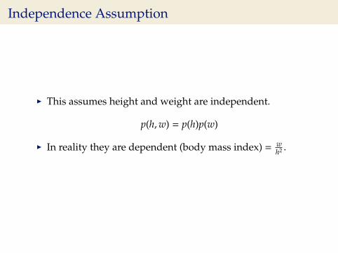
Independence Assumption

I This assumes height and weight are independent.

p(h,w) = p(h)p(w)

I In reality they are dependent (body mass index) = wh2 .

Sampling Two Dimensional Variables

Joint Distribution

w/k

g

h/m

Marginal Distributions

p(h)

p(w

)

Sampling Two Dimensional Variables

Joint Distribution

w/k

g

h/m

Marginal Distributions

p(h)

p(w

)

Sampling Two Dimensional Variables

Joint Distribution

w/k

g

h/m

Marginal Distributions

p(h)

p(w

)

Sampling Two Dimensional Variables

Joint Distribution

w/k

g

h/m

Marginal Distributions

p(h)

p(w

)

Sampling Two Dimensional Variables

Joint Distribution

w/k

g

h/m

Marginal Distributions

p(h)

p(w

)

Sampling Two Dimensional Variables

Joint Distribution

w/k

g

h/m

Marginal Distributions

p(h)

p(w

)

Sampling Two Dimensional Variables

Joint Distribution

w/k

g

h/m

Marginal Distributions

p(h)

p(w

)

Sampling Two Dimensional Variables

Joint Distribution

w/k

g

h/m

Marginal Distributions

p(h)

p(w

)

Sampling Two Dimensional Variables

Joint Distribution

w/k

g

h/m

Marginal Distributions

p(h)

p(w

)

Sampling Two Dimensional Variables

Joint Distribution

w/k

g

h/m

Marginal Distributions

p(h)

p(w

)

Sampling Two Dimensional Variables

Joint Distribution

w/k

g

h/m

Marginal Distributions

p(h)

p(w

)

Sampling Two Dimensional Variables

Joint Distribution

w/k

g

h/m

Marginal Distributions

p(h)

p(w

)

Sampling Two Dimensional Variables

Joint Distribution

w/k

g

h/m

Marginal Distributions

p(h)

p(w

)

Sampling Two Dimensional Variables

Joint Distribution

w/k

g

h/m

Marginal Distributions

p(h)

p(w

)

Sampling Two Dimensional Variables

Joint Distribution

w/k

g

h/m

Marginal Distributions

p(h)

p(w

)

Sampling Two Dimensional Variables

Joint Distribution

w/k

g

h/m

Marginal Distributions

p(h)

p(w

)

Sampling Two Dimensional Variables

Joint Distribution

w/k

g

h/m

Marginal Distributions

p(h)

p(w

)

Sampling Two Dimensional Variables

Joint Distribution

w/k

g

h/m

Marginal Distributions

p(h)

p(w

)

Sampling Two Dimensional Variables

Joint Distribution

w/k

g

h/m

Marginal Distributions

p(h)

p(w

)

Sampling Two Dimensional Variables

Joint Distribution

w/k

g

h/m

Marginal Distributions

p(h)

p(w

)

Sampling Two Dimensional Variables

Joint Distribution

w/k

g

h/m

Marginal Distributions

p(h)

p(w

)

Sampling Two Dimensional Variables

Joint Distribution

w/k

g

h/m

Marginal Distributions

p(h)

p(w

)

Sampling Two Dimensional Variables

Joint Distribution

w/k

g

h/m

Marginal Distributions

p(h)

p(w

)

Independent Gaussians

p(w, h) = p(w)p(h)

Independent Gaussians

p(w, h) =1√

2πσ21

√2πσ2

2

exp

−12

(w − µ1)2

σ21

+(h − µ2)2

σ22

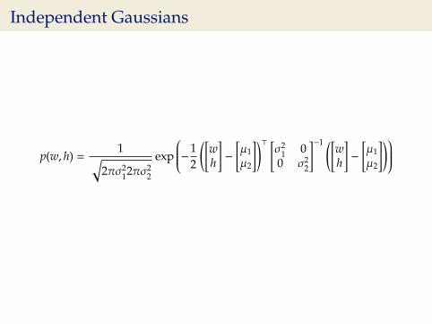
Independent Gaussians

p(w, h) =1√

2πσ212πσ2

2

exp

−12

([wh

]−

[µ1µ2

])> [σ2

1 00 σ2

2

]−1 ([wh

]−

[µ1µ2

])

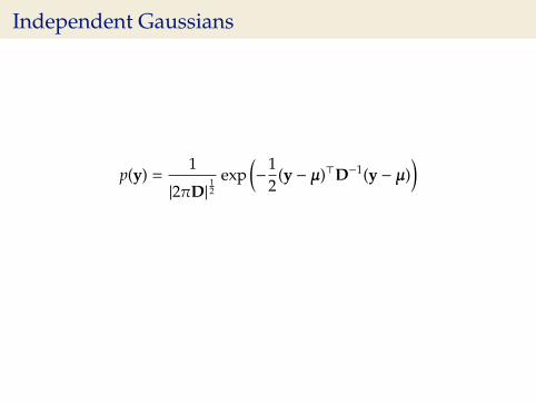
Independent Gaussians

p(y) =1

|2πD|12

exp(−

12

(y − µ)>D−1(y − µ))

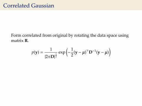
Correlated Gaussian

Form correlated from original by rotating the data space usingmatrix R.

p(y) =1

|2πD|12

exp(−

12

(y − µ)>D−1(y − µ))

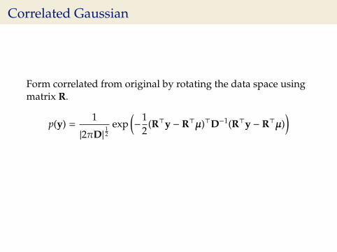
Correlated Gaussian

Form correlated from original by rotating the data space usingmatrix R.

p(y) =1

|2πD|12

exp(−

12

(R>y − R>µ)>D−1(R>y − R>µ))

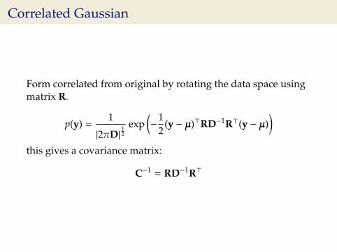
Correlated Gaussian

Form correlated from original by rotating the data space usingmatrix R.

p(y) =1

|2πD|12

exp(−

12

(y − µ)>RD−1R>(y − µ))

this gives a covariance matrix:

C−1 = RD−1R>

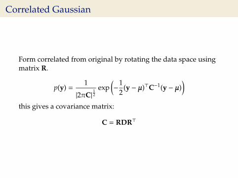
Correlated Gaussian

Form correlated from original by rotating the data space usingmatrix R.

p(y) =1

|2πC|12

exp(−

12

(y − µ)>C−1(y − µ))

this gives a covariance matrix:

C = RDR>

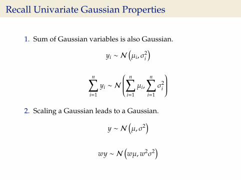
Recall Univariate Gaussian Properties

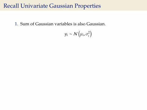
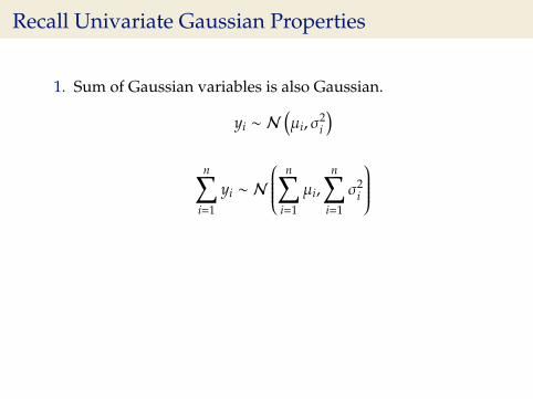
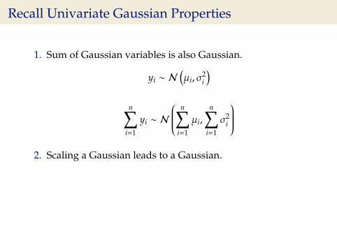
1. Sum of Gaussian variables is also Gaussian.

yi ∼ N(µi, σ

2i

)

n∑i=1

yi ∼ N

n∑i=1

µi,n∑

i=1

σ2i

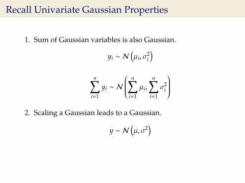
2. Scaling a Gaussian leads to a Gaussian.

y ∼ N(µ, σ2

)wy ∼ N

(wµ,w2σ2

)

Recall Univariate Gaussian Properties

1. Sum of Gaussian variables is also Gaussian.

yi ∼ N(µi, σ

2i

)n∑

i=1

yi ∼ N

n∑i=1

µi,n∑

i=1

σ2i

2. Scaling a Gaussian leads to a Gaussian.

y ∼ N(µ, σ2

)wy ∼ N

(wµ,w2σ2

)

Recall Univariate Gaussian Properties

1. Sum of Gaussian variables is also Gaussian.

yi ∼ N(µi, σ

2i

)n∑

i=1

yi ∼ N

n∑i=1

µi,n∑

i=1

σ2i

2. Scaling a Gaussian leads to a Gaussian.

y ∼ N(µ, σ2

)wy ∼ N

(wµ,w2σ2

)

Recall Univariate Gaussian Properties

1. Sum of Gaussian variables is also Gaussian.

yi ∼ N(µi, σ

2i

)n∑

i=1

yi ∼ N

n∑i=1

µi,n∑

i=1

σ2i

2. Scaling a Gaussian leads to a Gaussian.

y ∼ N(µ, σ2

)

wy ∼ N(wµ,w2σ2

)

Recall Univariate Gaussian Properties

1. Sum of Gaussian variables is also Gaussian.

yi ∼ N(µi, σ

2i

)n∑

i=1

yi ∼ N

n∑i=1

µi,n∑

i=1

σ2i

2. Scaling a Gaussian leads to a Gaussian.

y ∼ N(µ, σ2

)wy ∼ N

(wµ,w2σ2

)

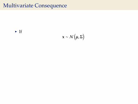
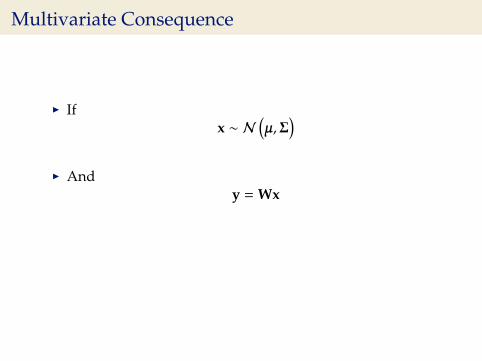
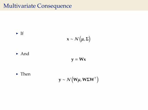
Multivariate Consequence

I Ifx ∼ N

(µ,Σ

)

I Andy = Wx

I Theny ∼ N

(Wµ,WΣW>

)

Multivariate Consequence

I Ifx ∼ N

(µ,Σ

)I And

y = Wx

I Theny ∼ N

(Wµ,WΣW>

)

Multivariate Consequence

I Ifx ∼ N

(µ,Σ

)I And

y = Wx

I Theny ∼ N

(Wµ,WΣW>

)

Sampling a Function

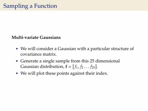
Multi-variate Gaussians

I We will consider a Gaussian with a particular structure ofcovariance matrix.

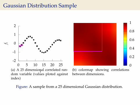
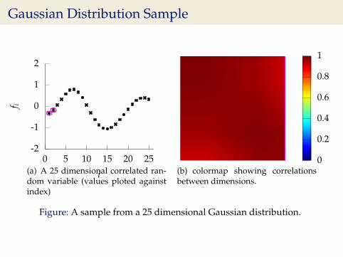
I Generate a single sample from this 25 dimensionalGaussian distribution, f =

[f1, f2 . . . f25

].

I We will plot these points against their index.

Gaussian Distribution Sample

-2

-1

0

1

2

0 5 10 15 20 25

f i

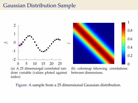
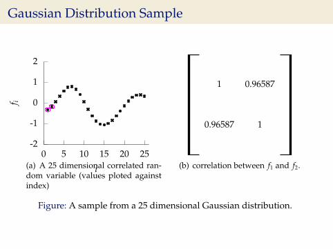
i(a) A 25 dimensional correlated ran-dom variable (values ploted againstindex)

ji

0

0.2

0.4

0.6

0.8

1

(b) colormap showing correlationsbetween dimensions.

Figure: A sample from a 25 dimensional Gaussian distribution.

Gaussian Distribution Sample

-2

-1

0

1

2

0 5 10 15 20 25

f i

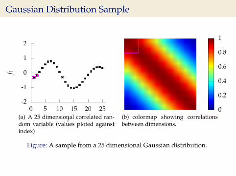
i(a) A 25 dimensional correlated ran-dom variable (values ploted againstindex)

ji

0

0.2

0.4

0.6

0.8

1

(b) colormap showing correlationsbetween dimensions.

Figure: A sample from a 25 dimensional Gaussian distribution.

Gaussian Distribution Sample

-2

-1

0

1

2

0 5 10 15 20 25

f i

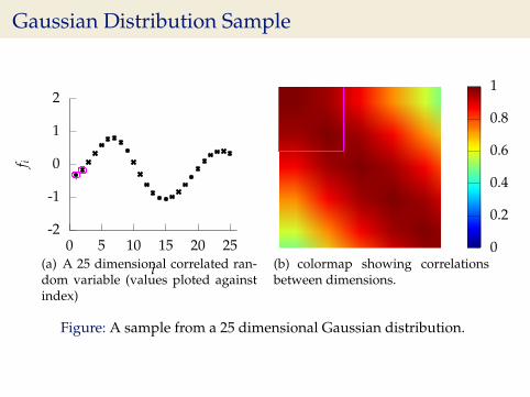
i(a) A 25 dimensional correlated ran-dom variable (values ploted againstindex)

0

0.2

0.4

0.6

0.8

1

(b) colormap showing correlationsbetween dimensions.

Figure: A sample from a 25 dimensional Gaussian distribution.

Gaussian Distribution Sample

-2

-1

0

1

2

0 5 10 15 20 25

f i

i(a) A 25 dimensional correlated ran-dom variable (values ploted againstindex)

0

0.2

0.4

0.6

0.8

1

(b) colormap showing correlationsbetween dimensions.

Figure: A sample from a 25 dimensional Gaussian distribution.

Gaussian Distribution Sample

-2

-1

0

1

2

0 5 10 15 20 25

f i

i(a) A 25 dimensional correlated ran-dom variable (values ploted againstindex)

0

0.2

0.4

0.6

0.8

1

(b) colormap showing correlationsbetween dimensions.

Figure: A sample from a 25 dimensional Gaussian distribution.

Gaussian Distribution Sample

-2

-1

0

1

2

0 5 10 15 20 25

f i

i(a) A 25 dimensional correlated ran-dom variable (values ploted againstindex)

0

0.2

0.4

0.6

0.8

1

(b) colormap showing correlationsbetween dimensions.

Figure: A sample from a 25 dimensional Gaussian distribution.

Gaussian Distribution Sample

-2

-1

0

1

2

0 5 10 15 20 25

f i

i(a) A 25 dimensional correlated ran-dom variable (values ploted againstindex)

0

0.2

0.4

0.6

0.8

1

(b) colormap showing correlationsbetween dimensions.

Figure: A sample from a 25 dimensional Gaussian distribution.

Gaussian Distribution Sample

-2

-1

0

1

2

0 5 10 15 20 25

f i

i(a) A 25 dimensional correlated ran-dom variable (values ploted againstindex)

1 0.96587

0.96587 1

(b) correlation between f1 and f2.

Figure: A sample from a 25 dimensional Gaussian distribution.

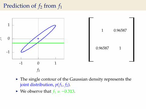
Prediction of f2 from f1

-1

0

1

-1 0 1

f 1

f2

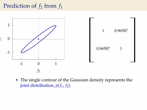
1 0.96587

0.96587 1

I The single contour of the Gaussian density represents thejoint distribution, p( f1, f2).

I We observe that f1 = −0.313.I Conditional density: p( f2| f1 = −0.313).

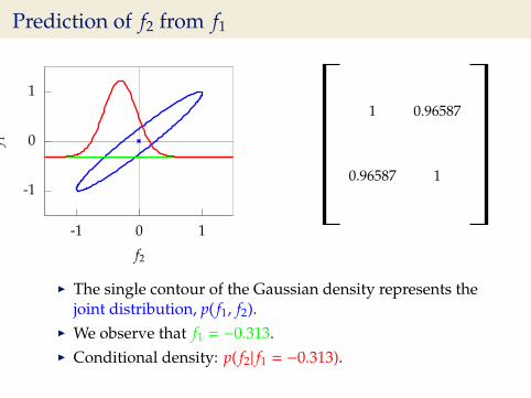
Prediction of f2 from f1

-1

0

1

-1 0 1

f 1

f2

1 0.96587

0.96587 1

I The single contour of the Gaussian density represents thejoint distribution, p( f1, f2).

I We observe that f1 = −0.313.

I Conditional density: p( f2| f1 = −0.313).

Prediction of f2 from f1

-1

0

1

-1 0 1

f 1

f2

1 0.96587

0.96587 1

I The single contour of the Gaussian density represents thejoint distribution, p( f1, f2).

I We observe that f1 = −0.313.I Conditional density: p( f2| f1 = −0.313).

Prediction of f2 from f1

-1

0

1

-1 0 1

f 1

f2

1 0.96587

0.96587 1

I The single contour of the Gaussian density represents thejoint distribution, p( f1, f2).

I We observe that f1 = −0.313.I Conditional density: p( f2| f1 = −0.313).

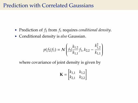
Prediction with Correlated Gaussians

I Prediction of f2 from f1 requires conditional density.I Conditional density is also Gaussian.

p( f2| f1) = N

f2|k1,2

k1,1f1, k2,2 −

k21,2

k1,1

where covariance of joint density is given by

K =

[k1,1 k1,2k2,1 k2,2

]

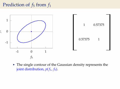
Prediction of f5 from f1

-1

0

1

-1 0 1

f 1

f5

1 0.57375

0.57375 1

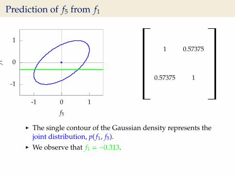
I The single contour of the Gaussian density represents thejoint distribution, p( f1, f5).

I We observe that f1 = −0.313.I Conditional density: p( f5| f1 = −0.313).

Prediction of f5 from f1

-1

0

1

-1 0 1

f 1

f5

1 0.57375

0.57375 1

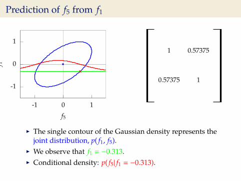
I The single contour of the Gaussian density represents thejoint distribution, p( f1, f5).

I We observe that f1 = −0.313.

I Conditional density: p( f5| f1 = −0.313).

Prediction of f5 from f1

-1

0

1

-1 0 1

f 1

f5

1 0.57375

0.57375 1

I The single contour of the Gaussian density represents thejoint distribution, p( f1, f5).

I We observe that f1 = −0.313.I Conditional density: p( f5| f1 = −0.313).

Prediction of f5 from f1

-1

0

1

-1 0 1

f 1

f5

1 0.57375

0.57375 1

I The single contour of the Gaussian density represents thejoint distribution, p( f1, f5).

I We observe that f1 = −0.313.I Conditional density: p( f5| f1 = −0.313).

Prediction with Correlated Gaussians

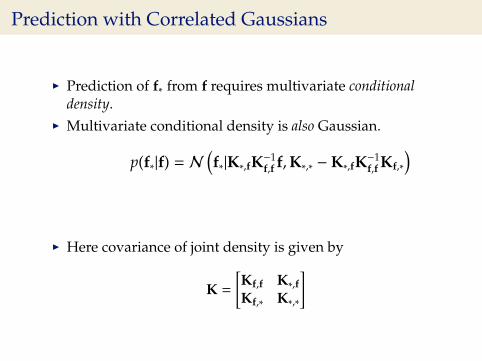
I Prediction of f∗ from f requires multivariate conditionaldensity.

I Multivariate conditional density is also Gaussian.

p(f∗|f) = N(f∗|K∗,fK−1

f,f f,K∗,∗ −K∗,fK−1f,f Kf,∗

)

I Here covariance of joint density is given by

K =

[Kf,f K∗,fKf,∗ K∗,∗

]

Prediction with Correlated Gaussians

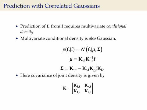
I Prediction of f∗ from f requires multivariate conditionaldensity.

I Multivariate conditional density is also Gaussian.

p(f∗|f) = N(f∗|µ,Σ

)µ = K∗,fK−1

f,f f

Σ = K∗,∗ −K∗,fK−1f,f Kf,∗

I Here covariance of joint density is given by

K =

[Kf,f K∗,fKf,∗ K∗,∗

]

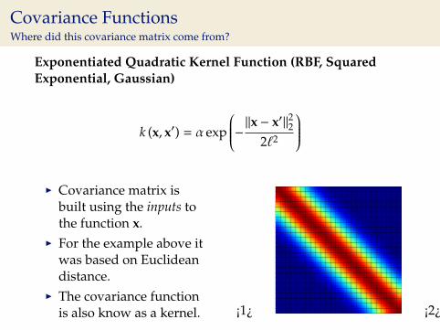
Covariance FunctionsWhere did this covariance matrix come from?

Exponentiated Quadratic Kernel Function (RBF, SquaredExponential, Gaussian)

k (x, x′) = α exp

−‖x − x′‖222`2

I Covariance matrix is

built using the inputs tothe function x.

I For the example above itwas based on Euclideandistance.

I The covariance functionis also know as a kernel. ¡1¿ ¡2¿

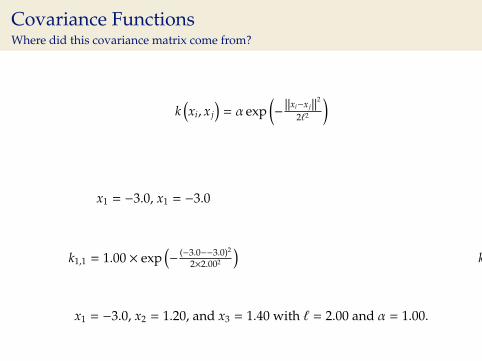
Covariance FunctionsWhere did this covariance matrix come from?

¡1¿

k(xi, x j

)= α exp

(−||xi−x j||

2

2`2

)

x1 = −3.0, x2 = 1.20, and x3 = 1.40 with ` = 2.00 and α = 1.00.

x1 = −3.0, x1 = −3.0

k1,1 = 1.00 × exp(−

(−3.0−−3.0)2

2×2.002

)

¡2¿

1.00

k(xi, x j

)= α exp

(−||xi−x j||

2

2`2

)

x1 = −3.0, x2 = 1.20, and x3 = 1.40 with ` = 2.00 and α = 1.00.

x1 = −3.0, x1 = −3.0

k1,1 = 1.00 × exp(−

(−3.0−−3.0)2

2×2.002

)

¡3¿

1.00

k(xi, x j

)= α exp

(−||xi−x j||

2

2`2

)

x1 = −3.0, x2 = 1.20, and x3 = 1.40 with ` = 2.00 and α = 1.00.

x2 = 1.20, x1 = −3.0

k2,1 = 1.00 × exp(−

(1.20−−3.0)2

2×2.002

)

¡4¿

1.00

0.110

k(xi, x j

)= α exp

(−||xi−x j||

2

2`2

)

x1 = −3.0, x2 = 1.20, and x3 = 1.40 with ` = 2.00 and α = 1.00.

x2 = 1.20, x1 = −3.0

k2,1 = 1.00 × exp(−

(1.20−−3.0)2

2×2.002

)

¡5¿

1.00 0.110

0.110

k(xi, x j

)= α exp

(−||xi−x j||

2

2`2

)

x1 = −3.0, x2 = 1.20, and x3 = 1.40 with ` = 2.00 and α = 1.00.

x2 = 1.20, x1 = −3.0

k2,1 = 1.00 × exp(−

(1.20−−3.0)2

2×2.002

)

¡6¿

1.00 0.110

0.110

k(xi, x j

)= α exp

(−||xi−x j||

2

2`2

)

x1 = −3.0, x2 = 1.20, and x3 = 1.40 with ` = 2.00 and α = 1.00.

x2 = 1.20, x2 = 1.20

k2,2 = 1.00 × exp(−

(1.20−1.20)2

2×2.002

)

¡7¿

1.00 0.110

0.110 1.00

k(xi, x j

)= α exp

(−||xi−x j||

2

2`2

)

x1 = −3.0, x2 = 1.20, and x3 = 1.40 with ` = 2.00 and α = 1.00.

x2 = 1.20, x2 = 1.20

k2,2 = 1.00 × exp(−

(1.20−1.20)2

2×2.002

)

¡8¿

1.00 0.110

0.110 1.00

k(xi, x j

)= α exp

(−||xi−x j||

2

2`2

)

x1 = −3.0, x2 = 1.20, and x3 = 1.40 with ` = 2.00 and α = 1.00.

x3 = 1.40, x1 = −3.0

k3,1 = 1.00 × exp(−

(1.40−−3.0)2

2×2.002

)

¡9¿

1.00 0.110

0.110 1.00

0.0889

k(xi, x j

)= α exp

(−||xi−x j||

2

2`2

)

x1 = −3.0, x2 = 1.20, and x3 = 1.40 with ` = 2.00 and α = 1.00.

x3 = 1.40, x1 = −3.0

k3,1 = 1.00 × exp(−

(1.40−−3.0)2

2×2.002

)

¡10¿

1.00 0.110 0.0889

0.110 1.00

0.0889

k(xi, x j

)= α exp

(−||xi−x j||

2

2`2

)

x1 = −3.0, x2 = 1.20, and x3 = 1.40 with ` = 2.00 and α = 1.00.

x3 = 1.40, x1 = −3.0

k3,1 = 1.00 × exp(−

(1.40−−3.0)2

2×2.002

)

¡11¿

1.00 0.110 0.0889

0.110 1.00

0.0889

k(xi, x j

)= α exp

(−||xi−x j||

2

2`2

)

x1 = −3.0, x2 = 1.20, and x3 = 1.40 with ` = 2.00 and α = 1.00.

x3 = 1.40, x2 = 1.20

k3,2 = 1.00 × exp(−

(1.40−1.20)2

2×2.002

)

¡12¿

1.00 0.110 0.0889

0.110 1.00

0.0889 0.995

k(xi, x j

)= α exp

(−||xi−x j||

2

2`2

)

x1 = −3.0, x2 = 1.20, and x3 = 1.40 with ` = 2.00 and α = 1.00.

x3 = 1.40, x2 = 1.20

k3,2 = 1.00 × exp(−

(1.40−1.20)2

2×2.002

)

¡13¿

1.00 0.110 0.0889

0.110 1.00 0.995

0.0889 0.995

k(xi, x j

)= α exp

(−||xi−x j||

2

2`2

)

x1 = −3.0, x2 = 1.20, and x3 = 1.40 with ` = 2.00 and α = 1.00.

x3 = 1.40, x2 = 1.20

k3,2 = 1.00 × exp(−

(1.40−1.20)2

2×2.002

)

¡14¿

1.00 0.110 0.0889

0.110 1.00 0.995

0.0889 0.995

k(xi, x j

)= α exp

(−||xi−x j||

2

2`2

)

x1 = −3.0, x2 = 1.20, and x3 = 1.40 with ` = 2.00 and α = 1.00.

x3 = 1.40, x3 = 1.40

k3,3 = 1.00 × exp(−

(1.40−1.40)2

2×2.002

)

¡15¿

1.00 0.110 0.0889

0.110 1.00 0.995

0.0889 0.995 1.00

k(xi, x j

)= α exp

(−||xi−x j||

2

2`2

)

x1 = −3.0, x2 = 1.20, and x3 = 1.40 with ` = 2.00 and α = 1.00.

x3 = 1.40, x3 = 1.40

k3,3 = 1.00 × exp(−

(1.40−1.40)2

2×2.002

)

¡16¿

k(xi, x j

)= α exp

(−||xi−x j||

2

2`2

)

x1 = −3.0, x2 = 1.20, and x3 = 1.40 with ` = 2.00 and α = 1.00.

x3 = 1.40, x3 = 1.40

k3,3 = 1.00 × exp(−

(1.40−1.40)2

2×2.002

)

¡17¿

k(xi, x j

)= α exp

(−||xi−x j||

2

2`2

)

x1 = −3, x2 = 1.2, x3 = 1.4, and x4 = 2.0 with ` = 2.0 and α = 1.0.

x1 = −3, x1 = −3

k1,1 = 1.0 × exp(−

(−3−−3)2

2×2.02

)

¡18¿

1.0

k(xi, x j

)= α exp

(−||xi−x j||

2

2`2

)

x1 = −3, x2 = 1.2, x3 = 1.4, and x4 = 2.0 with ` = 2.0 and α = 1.0.

x1 = −3, x1 = −3

k1,1 = 1.0 × exp(−

(−3−−3)2

2×2.02

)

¡19¿

1.0

k(xi, x j

)= α exp

(−||xi−x j||

2

2`2

)

x1 = −3, x2 = 1.2, x3 = 1.4, and x4 = 2.0 with ` = 2.0 and α = 1.0.

x2 = 1.2, x1 = −3

k2,1 = 1.0 × exp(−

(1.2−−3)2

2×2.02

)

¡20¿

1.0

0.11

k(xi, x j

)= α exp

(−||xi−x j||

2

2`2

)

x1 = −3, x2 = 1.2, x3 = 1.4, and x4 = 2.0 with ` = 2.0 and α = 1.0.

x2 = 1.2, x1 = −3

k2,1 = 1.0 × exp(−

(1.2−−3)2

2×2.02

)

¡21¿

1.0 0.11

0.11

k(xi, x j

)= α exp

(−||xi−x j||

2

2`2

)

x1 = −3, x2 = 1.2, x3 = 1.4, and x4 = 2.0 with ` = 2.0 and α = 1.0.

x2 = 1.2, x1 = −3

k2,1 = 1.0 × exp(−

(1.2−−3)2

2×2.02

)

¡22¿

1.0 0.11

0.11

k(xi, x j

)= α exp

(−||xi−x j||

2

2`2

)

x1 = −3, x2 = 1.2, x3 = 1.4, and x4 = 2.0 with ` = 2.0 and α = 1.0.

x2 = 1.2, x2 = 1.2

k2,2 = 1.0 × exp(−

(1.2−1.2)2

2×2.02

)

¡23¿

1.0 0.11

0.11 1.0

k(xi, x j

)= α exp

(−||xi−x j||

2

2`2

)

x1 = −3, x2 = 1.2, x3 = 1.4, and x4 = 2.0 with ` = 2.0 and α = 1.0.

x2 = 1.2, x2 = 1.2

k2,2 = 1.0 × exp(−

(1.2−1.2)2

2×2.02

)

¡24¿

1.0 0.11

0.11 1.0

k(xi, x j

)= α exp

(−||xi−x j||

2

2`2

)

x1 = −3, x2 = 1.2, x3 = 1.4, and x4 = 2.0 with ` = 2.0 and α = 1.0.

x3 = 1.4, x1 = −3

k3,1 = 1.0 × exp(−

(1.4−−3)2

2×2.02

)

¡25¿

1.0 0.11

0.11 1.0

0.089

k(xi, x j

)= α exp

(−||xi−x j||

2

2`2

)

x1 = −3, x2 = 1.2, x3 = 1.4, and x4 = 2.0 with ` = 2.0 and α = 1.0.

x3 = 1.4, x1 = −3

k3,1 = 1.0 × exp(−

(1.4−−3)2

2×2.02

)

¡26¿

1.0 0.11 0.089

0.11 1.0

0.089

k(xi, x j

)= α exp

(−||xi−x j||

2

2`2

)

x1 = −3, x2 = 1.2, x3 = 1.4, and x4 = 2.0 with ` = 2.0 and α = 1.0.

x3 = 1.4, x1 = −3

k3,1 = 1.0 × exp(−

(1.4−−3)2

2×2.02

)

¡27¿

1.0 0.11 0.089

0.11 1.0

0.089

k(xi, x j

)= α exp

(−||xi−x j||

2

2`2

)

x1 = −3, x2 = 1.2, x3 = 1.4, and x4 = 2.0 with ` = 2.0 and α = 1.0.

x3 = 1.4, x2 = 1.2

k3,2 = 1.0 × exp(−

(1.4−1.2)2

2×2.02

)

¡28¿

1.0 0.11 0.089

0.11 1.0

0.089 1.0

k(xi, x j

)= α exp

(−||xi−x j||

2

2`2

)

x1 = −3, x2 = 1.2, x3 = 1.4, and x4 = 2.0 with ` = 2.0 and α = 1.0.

x3 = 1.4, x2 = 1.2

k3,2 = 1.0 × exp(−

(1.4−1.2)2

2×2.02

)

¡29¿

1.0 0.11 0.089

0.11 1.0 1.0

0.089 1.0

k(xi, x j

)= α exp

(−||xi−x j||

2

2`2

)

x1 = −3, x2 = 1.2, x3 = 1.4, and x4 = 2.0 with ` = 2.0 and α = 1.0.

x3 = 1.4, x2 = 1.2

k3,2 = 1.0 × exp(−

(1.4−1.2)2

2×2.02

)

¡30¿

1.0 0.11 0.089

0.11 1.0 1.0

0.089 1.0

k(xi, x j

)= α exp

(−||xi−x j||

2

2`2

)

x1 = −3, x2 = 1.2, x3 = 1.4, and x4 = 2.0 with ` = 2.0 and α = 1.0.

x3 = 1.4, x3 = 1.4

k3,3 = 1.0 × exp(−

(1.4−1.4)2

2×2.02

)

¡31¿

1.0 0.11 0.089

0.11 1.0 1.0

0.089 1.0 1.0

k(xi, x j

)= α exp

(−||xi−x j||

2

2`2

)

x1 = −3, x2 = 1.2, x3 = 1.4, and x4 = 2.0 with ` = 2.0 and α = 1.0.

x3 = 1.4, x3 = 1.4

k3,3 = 1.0 × exp(−

(1.4−1.4)2

2×2.02

)

¡32¿

1.0 0.11 0.089

0.11 1.0 1.0

0.089 1.0 1.0

k(xi, x j

)= α exp

(−||xi−x j||

2

2`2

)

x1 = −3, x2 = 1.2, x3 = 1.4, and x4 = 2.0 with ` = 2.0 and α = 1.0.

x4 = 2.0, x1 = −3

k4,1 = 1.0 × exp(−

(2.0−−3)2

2×2.02

)

¡33¿

1.0 0.11 0.089

0.11 1.0 1.0

0.089 1.0 1.0

0.044

k(xi, x j

)= α exp

(−||xi−x j||

2

2`2

)

x1 = −3, x2 = 1.2, x3 = 1.4, and x4 = 2.0 with ` = 2.0 and α = 1.0.

x4 = 2.0, x1 = −3

k4,1 = 1.0 × exp(−

(2.0−−3)2

2×2.02

)

¡34¿

1.0 0.11 0.089 0.044

0.11 1.0 1.0

0.089 1.0 1.0

0.044

k(xi, x j

)= α exp

(−||xi−x j||

2

2`2

)

x1 = −3, x2 = 1.2, x3 = 1.4, and x4 = 2.0 with ` = 2.0 and α = 1.0.

x4 = 2.0, x1 = −3

k4,1 = 1.0 × exp(−

(2.0−−3)2

2×2.02

)

¡35¿

1.0 0.11 0.089 0.044

0.11 1.0 1.0

0.089 1.0 1.0

0.044

k(xi, x j

)= α exp

(−||xi−x j||

2

2`2

)

x1 = −3, x2 = 1.2, x3 = 1.4, and x4 = 2.0 with ` = 2.0 and α = 1.0.

x4 = 2.0, x2 = 1.2

k4,2 = 1.0 × exp(−

(2.0−1.2)2

2×2.02

)

¡36¿

1.0 0.11 0.089 0.044

0.11 1.0 1.0

0.089 1.0 1.0

0.044 0.92

k(xi, x j

)= α exp

(−||xi−x j||

2

2`2

)

x1 = −3, x2 = 1.2, x3 = 1.4, and x4 = 2.0 with ` = 2.0 and α = 1.0.

x4 = 2.0, x2 = 1.2

k4,2 = 1.0 × exp(−

(2.0−1.2)2

2×2.02

)

¡37¿

1.0 0.11 0.089 0.044

0.11 1.0 1.0 0.92

0.089 1.0 1.0

0.044 0.92

k(xi, x j

)= α exp

(−||xi−x j||

2

2`2

)

x1 = −3, x2 = 1.2, x3 = 1.4, and x4 = 2.0 with ` = 2.0 and α = 1.0.

x4 = 2.0, x2 = 1.2

k4,2 = 1.0 × exp(−

(2.0−1.2)2

2×2.02

)

¡38¿

1.0 0.11 0.089 0.044

0.11 1.0 1.0 0.92

0.089 1.0 1.0

0.044 0.92

k(xi, x j

)= α exp

(−||xi−x j||

2

2`2

)

x1 = −3, x2 = 1.2, x3 = 1.4, and x4 = 2.0 with ` = 2.0 and α = 1.0.

x4 = 2.0, x3 = 1.4

k4,3 = 1.0 × exp(−

(2.0−1.4)2

2×2.02

)

¡39¿

1.0 0.11 0.089 0.044

0.11 1.0 1.0 0.92

0.089 1.0 1.0

0.044 0.92 0.96

k(xi, x j

)= α exp

(−||xi−x j||

2

2`2

)

x1 = −3, x2 = 1.2, x3 = 1.4, and x4 = 2.0 with ` = 2.0 and α = 1.0.

x4 = 2.0, x3 = 1.4

k4,3 = 1.0 × exp(−

(2.0−1.4)2

2×2.02

)

¡40¿

1.0 0.11 0.089 0.044

0.11 1.0 1.0 0.92

0.089 1.0 1.0 0.96

0.044 0.92 0.96

k(xi, x j

)= α exp

(−||xi−x j||

2

2`2

)

x1 = −3, x2 = 1.2, x3 = 1.4, and x4 = 2.0 with ` = 2.0 and α = 1.0.

x4 = 2.0, x3 = 1.4

k4,3 = 1.0 × exp(−

(2.0−1.4)2

2×2.02

)

¡41¿

1.0 0.11 0.089 0.044

0.11 1.0 1.0 0.92

0.089 1.0 1.0 0.96

0.044 0.92 0.96

k(xi, x j

)= α exp

(−||xi−x j||

2

2`2

)

x1 = −3, x2 = 1.2, x3 = 1.4, and x4 = 2.0 with ` = 2.0 and α = 1.0.

x4 = 2.0, x4 = 2.0

k4,4 = 1.0 × exp(−

(2.0−2.0)2

2×2.02

)

¡42¿

1.0 0.11 0.089 0.044

0.11 1.0 1.0 0.92

0.089 1.0 1.0 0.96

0.044 0.92 0.96 1.0

k(xi, x j

)= α exp

(−||xi−x j||

2

2`2

)

x1 = −3, x2 = 1.2, x3 = 1.4, and x4 = 2.0 with ` = 2.0 and α = 1.0.

x4 = 2.0, x4 = 2.0

k4,4 = 1.0 × exp(−

(2.0−2.0)2

2×2.02

)

¡43¿

k(xi, x j

)= α exp

(−||xi−x j||

2

2`2

)

x1 = −3, x2 = 1.2, x3 = 1.4, and x4 = 2.0 with ` = 2.0 and α = 1.0.

x4 = 2.0, x4 = 2.0

k4,4 = 1.0 × exp(−

(2.0−2.0)2

2×2.02

)

¡44¿

k(xi, x j

)= α exp

(−||xi−x j||

2

2`2

)

x1 = −3.0, x2 = 1.20, and x3 = 1.40 with ` = 5.00 and α = 4.00.

x1 = −3.0, x1 = −3.0

k1,1 = 4.00 × exp(−

(−3.0−−3.0)2

2×5.002

)

¡45¿

4.00

k(xi, x j

)= α exp

(−||xi−x j||

2

2`2

)

x1 = −3.0, x2 = 1.20, and x3 = 1.40 with ` = 5.00 and α = 4.00.

x1 = −3.0, x1 = −3.0

k1,1 = 4.00 × exp(−

(−3.0−−3.0)2

2×5.002

)

¡46¿

4.00

k(xi, x j

)= α exp

(−||xi−x j||

2

2`2

)

x1 = −3.0, x2 = 1.20, and x3 = 1.40 with ` = 5.00 and α = 4.00.

x2 = 1.20, x1 = −3.0

k2,1 = 4.00 × exp(−

(1.20−−3.0)2

2×5.002

)

¡47¿

4.00

2.81

k(xi, x j

)= α exp

(−||xi−x j||

2

2`2

)

x1 = −3.0, x2 = 1.20, and x3 = 1.40 with ` = 5.00 and α = 4.00.

x2 = 1.20, x1 = −3.0

k2,1 = 4.00 × exp(−

(1.20−−3.0)2

2×5.002

)

¡48¿

4.00 2.81

2.81

k(xi, x j

)= α exp

(−||xi−x j||

2

2`2

)

x1 = −3.0, x2 = 1.20, and x3 = 1.40 with ` = 5.00 and α = 4.00.

x2 = 1.20, x1 = −3.0

k2,1 = 4.00 × exp(−

(1.20−−3.0)2

2×5.002

)

¡49¿

4.00 2.81

2.81

k(xi, x j

)= α exp

(−||xi−x j||

2

2`2

)

x1 = −3.0, x2 = 1.20, and x3 = 1.40 with ` = 5.00 and α = 4.00.

x2 = 1.20, x2 = 1.20

k2,2 = 4.00 × exp(−

(1.20−1.20)2

2×5.002

)

¡50¿

4.00 2.81

2.81 4.00

k(xi, x j

)= α exp

(−||xi−x j||

2

2`2

)

x1 = −3.0, x2 = 1.20, and x3 = 1.40 with ` = 5.00 and α = 4.00.

x2 = 1.20, x2 = 1.20

k2,2 = 4.00 × exp(−

(1.20−1.20)2

2×5.002

)

¡51¿

4.00 2.81

2.81 4.00

k(xi, x j

)= α exp

(−||xi−x j||

2

2`2

)

x1 = −3.0, x2 = 1.20, and x3 = 1.40 with ` = 5.00 and α = 4.00.

x3 = 1.40, x1 = −3.0

k3,1 = 4.00 × exp(−

(1.40−−3.0)2

2×5.002

)

¡52¿

4.00 2.81

2.81 4.00

2.72

k(xi, x j

)= α exp

(−||xi−x j||

2

2`2

)

x1 = −3.0, x2 = 1.20, and x3 = 1.40 with ` = 5.00 and α = 4.00.

x3 = 1.40, x1 = −3.0

k3,1 = 4.00 × exp(−

(1.40−−3.0)2

2×5.002

)

¡53¿

4.00 2.81 2.72

2.81 4.00

2.72

k(xi, x j

)= α exp

(−||xi−x j||

2

2`2

)

x1 = −3.0, x2 = 1.20, and x3 = 1.40 with ` = 5.00 and α = 4.00.

x3 = 1.40, x1 = −3.0

k3,1 = 4.00 × exp(−

(1.40−−3.0)2

2×5.002

)

¡54¿

4.00 2.81 2.72

2.81 4.00

2.72

k(xi, x j

)= α exp

(−||xi−x j||

2

2`2

)

x1 = −3.0, x2 = 1.20, and x3 = 1.40 with ` = 5.00 and α = 4.00.

x3 = 1.40, x2 = 1.20

k3,2 = 4.00 × exp(−

(1.40−1.20)2

2×5.002

)

¡55¿

4.00 2.81 2.72

2.81 4.00

2.72 4.00

k(xi, x j

)= α exp

(−||xi−x j||

2

2`2

)

x1 = −3.0, x2 = 1.20, and x3 = 1.40 with ` = 5.00 and α = 4.00.

x3 = 1.40, x2 = 1.20

k3,2 = 4.00 × exp(−

(1.40−1.20)2

2×5.002

)

¡56¿

4.00 2.81 2.72

2.81 4.00 4.00

2.72 4.00

k(xi, x j

)= α exp

(−||xi−x j||

2

2`2

)

x1 = −3.0, x2 = 1.20, and x3 = 1.40 with ` = 5.00 and α = 4.00.

x3 = 1.40, x2 = 1.20

k3,2 = 4.00 × exp(−

(1.40−1.20)2

2×5.002

)

¡57¿

4.00 2.81 2.72

2.81 4.00 4.00

2.72 4.00

k(xi, x j

)= α exp

(−||xi−x j||

2

2`2

)

x1 = −3.0, x2 = 1.20, and x3 = 1.40 with ` = 5.00 and α = 4.00.

x3 = 1.40, x3 = 1.40

k3,3 = 4.00 × exp(−

(1.40−1.40)2

2×5.002

)

¡58¿

4.00 2.81 2.72

2.81 4.00 4.00

2.72 4.00 4.00

k(xi, x j

)= α exp

(−||xi−x j||

2

2`2

)

x1 = −3.0, x2 = 1.20, and x3 = 1.40 with ` = 5.00 and α = 4.00.

x3 = 1.40, x3 = 1.40

k3,3 = 4.00 × exp(−

(1.40−1.40)2

2×5.002

)

¡59¿

k(xi, x j

)= α exp

(−||xi−x j||

2

2`2

)

x1 = −3.0, x2 = 1.20, and x3 = 1.40 with ` = 5.00 and α = 4.00.

x3 = 1.40, x3 = 1.40

k3,3 = 4.00 × exp(−

(1.40−1.40)2

2×5.002

)

Outline

The Gaussian Density

Covariance from Basis Functions

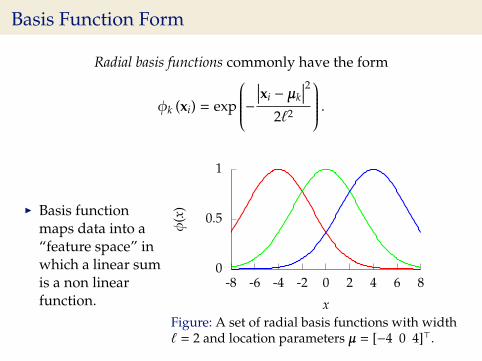
Basis Function Form

Radial basis functions commonly have the form

φk (xi) = exp

−∣∣∣xi − µk

∣∣∣22`2

.

I Basis functionmaps data into a“feature space” inwhich a linear sumis a non linearfunction.

0

0.5

1

-8 -6 -4 -2 0 2 4 6 8

φ(x

)

xFigure: A set of radial basis functions with width` = 2 and location parameters µ = [−4 0 4]>.

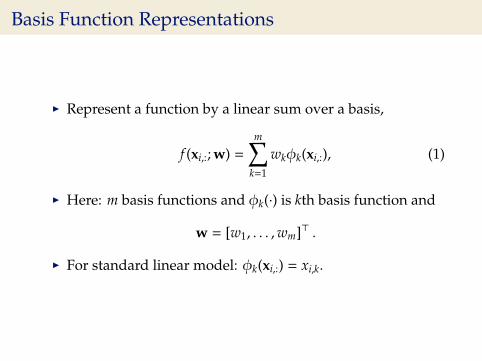
Basis Function Representations

I Represent a function by a linear sum over a basis,

f (xi,:; w) =

m∑k=1

wkφk(xi,:), (1)

I Here: m basis functions and φk(·) is kth basis function and

w = [w1, . . . ,wm]> .

I For standard linear model: φk(xi,:) = xi,k.

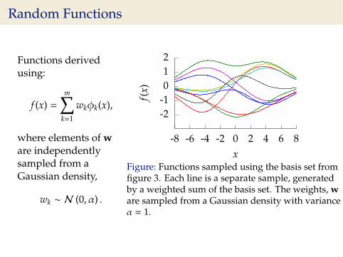
Random Functions

Functions derivedusing:

f (x) =

m∑k=1

wkφk(x),

where elements of ware independentlysampled from aGaussian density,

wk ∼ N (0, α) .

-2-1012

-8 -6 -4 -2 0 2 4 6 8f(

x)x

Figure: Functions sampled using the basis set fromfigure 3. Each line is a separate sample, generatedby a weighted sum of the basis set. The weights, ware sampled from a Gaussian density with varianceα = 1.

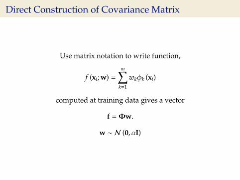
Direct Construction of Covariance Matrix

Use matrix notation to write function,

f (xi; w) =

m∑k=1

wkφk (xi)

Direct Construction of Covariance Matrix

Use matrix notation to write function,

f (xi; w) =

m∑k=1

wkφk (xi)

computed at training data gives a vector

f =Φw.

Direct Construction of Covariance Matrix

Use matrix notation to write function,

f (xi; w) =

m∑k=1

wkφk (xi)

computed at training data gives a vector

f =Φw.

w ∼ N (0, αI)

Direct Construction of Covariance Matrix

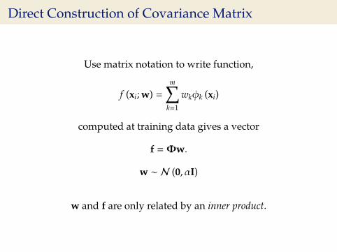
Use matrix notation to write function,

f (xi; w) =

m∑k=1

wkφk (xi)

computed at training data gives a vector

f =Φw.

w ∼ N (0, αI)

w and f are only related by an inner product.

Direct Construction of Covariance Matrix

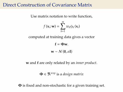
Use matrix notation to write function,

f (xi; w) =

m∑k=1

wkφk (xi)

computed at training data gives a vector

f =Φw.

w ∼ N (0, αI)

w and f are only related by an inner product.

Φ ∈ <n×p is a design matrix

Direct Construction of Covariance Matrix

Use matrix notation to write function,

f (xi; w) =

m∑k=1

wkφk (xi)

computed at training data gives a vector

f =Φw.

w ∼ N (0, αI)

w and f are only related by an inner product.

Φ ∈ <n×p is a design matrix

Φ is fixed and non-stochastic for a given training set.

Direct Construction of Covariance Matrix

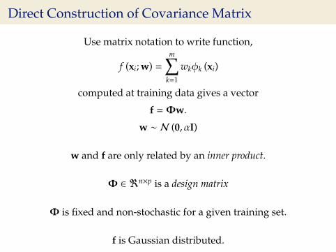
Use matrix notation to write function,

f (xi; w) =

m∑k=1

wkφk (xi)

computed at training data gives a vector

f =Φw.

w ∼ N (0, αI)

w and f are only related by an inner product.

Φ ∈ <n×p is a design matrix

Φ is fixed and non-stochastic for a given training set.

f is Gaussian distributed.

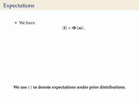
Expectations

I We have〈f〉 =Φ 〈w〉 .

I Prior mean of w was zero giving

〈f〉 = 0.

I Prior covariance of f is

K =⟨ff>

⟩− 〈f〉 〈f〉>

We use 〈·〉 to denote expectations under prior distributions.

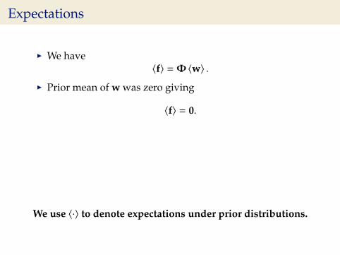
Expectations

I We have〈f〉 =Φ 〈w〉 .

I Prior mean of w was zero giving

〈f〉 = 0.

I Prior covariance of f is

K =⟨ff>

⟩− 〈f〉 〈f〉>

We use 〈·〉 to denote expectations under prior distributions.

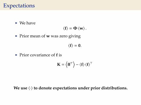
Expectations

I We have〈f〉 =Φ 〈w〉 .

I Prior mean of w was zero giving

〈f〉 = 0.

I Prior covariance of f is

K =⟨ff>

⟩− 〈f〉 〈f〉>

We use 〈·〉 to denote expectations under prior distributions.

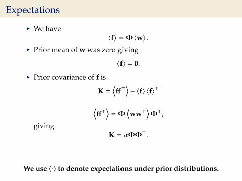
Expectations

I We have〈f〉 =Φ 〈w〉 .

I Prior mean of w was zero giving

〈f〉 = 0.

I Prior covariance of f is

K =⟨ff>

⟩− 〈f〉 〈f〉>

⟨ff>

⟩=Φ

⟨ww>

⟩Φ>,

givingK = αΦΦ>.

We use 〈·〉 to denote expectations under prior distributions.

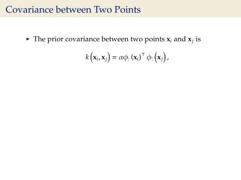
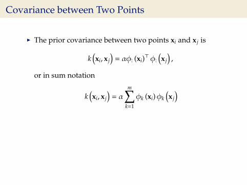
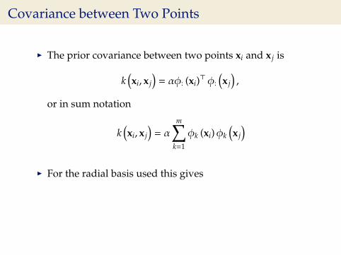
Covariance between Two Points

I The prior covariance between two points xi and x j is

k(xi, x j

)= αφ: (xi)

> φ:

(x j

),

or in sum notation

k(xi, x j

)= α

m∑k=1

φk (xi)φk

(x j

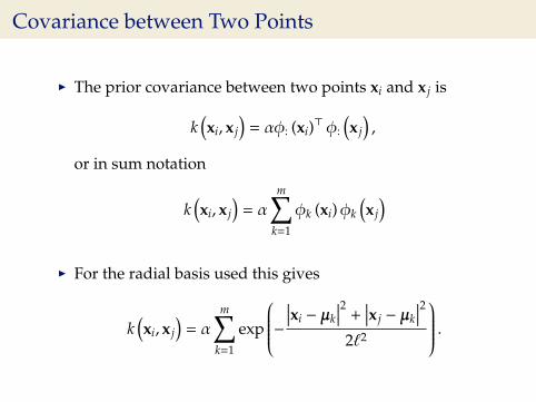
)I For the radial basis used this gives

k(xi, x j

)= α

m∑k=1

exp

−∣∣∣xi − µk

∣∣∣2 +∣∣∣x j − µk

∣∣∣22`2

.

Covariance between Two Points

I The prior covariance between two points xi and x j is

k(xi, x j

)= αφ: (xi)

> φ:

(x j

),

or in sum notation

k(xi, x j

)= α

m∑k=1

φk (xi)φk

(x j

)

I For the radial basis used this gives

k(xi, x j

)= α

m∑k=1

exp

−∣∣∣xi − µk

∣∣∣2 +∣∣∣x j − µk

∣∣∣22`2

.

Covariance between Two Points

I The prior covariance between two points xi and x j is

k(xi, x j

)= αφ: (xi)

> φ:

(x j

),

or in sum notation

k(xi, x j

)= α

m∑k=1

φk (xi)φk

(x j

)I For the radial basis used this gives

k(xi, x j

)= α

m∑k=1

exp

−∣∣∣xi − µk

∣∣∣2 +∣∣∣x j − µk

∣∣∣22`2

.

Covariance between Two Points

I The prior covariance between two points xi and x j is

k(xi, x j

)= αφ: (xi)

> φ:

(x j

),

or in sum notation

k(xi, x j

)= α

m∑k=1

φk (xi)φk

(x j

)I For the radial basis used this gives

k(xi, x j

)= α

m∑k=1

exp

−∣∣∣xi − µk

∣∣∣2 +∣∣∣x j − µk

∣∣∣22`2

.

Covariance Functions

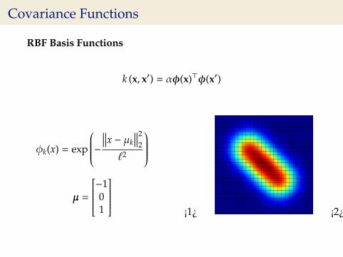
RBF Basis Functions

k (x, x′) = αφ(x)>φ(x′)

φk(x) = exp

−∥∥∥x − µk

∥∥∥22

`2

µ =

−101

¡1¿ ¡2¿

-3-2-10123

-3 -2 -1 0 1 2 3

Selecting Number and Location of Basis

I Need to choose1. location of centers2. number of basis functions

Restrict analysis to 1-D input, x.I Consider uniform spacing over a region:

k(xi, x j

)= αφk(xi)>φk(x j)

Selecting Number and Location of Basis

I Need to choose1. location of centers2. number of basis functions

Restrict analysis to 1-D input, x.I Consider uniform spacing over a region:

k(xi, x j

)= α

m∑k=1

φk(xi)φk(x j)

Selecting Number and Location of Basis

I Need to choose1. location of centers2. number of basis functions

Restrict analysis to 1-D input, x.I Consider uniform spacing over a region:

k(xi, x j

)= α

m∑k=1

exp(−

(xi − µk)2

2`2

)exp

− (x j − µk)2

2`2

Selecting Number and Location of Basis

I Need to choose1. location of centers2. number of basis functions

Restrict analysis to 1-D input, x.I Consider uniform spacing over a region:

k(xi, x j

)= α

m∑k=1

exp

− (xi − µk)2

2`2 −(x j − µk)2

2`2

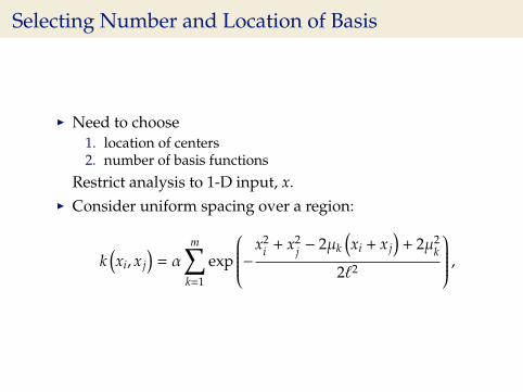
Selecting Number and Location of Basis

I Need to choose1. location of centers2. number of basis functions

Restrict analysis to 1-D input, x.I Consider uniform spacing over a region:

k(xi, x j

)= α

m∑k=1

exp

−x2i + x2

j − 2µk

(xi + x j

)+ 2µ2

k

2`2

,

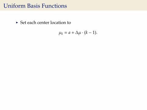
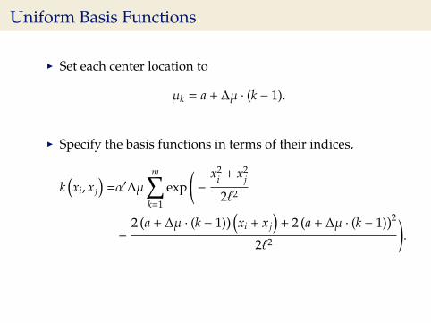
Uniform Basis Functions

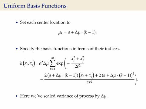
I Set each center location to

µk = a + ∆µ · (k − 1).

I Specify the basis functions in terms of their indices,

k(xi, x j

)=α′∆µ

m∑k=1

exp(−

x2i + x2

j

2`2

−

2(a + ∆µ · (k − 1)

) (xi + x j

)+ 2

(a + ∆µ · (k − 1)

)2

2`2

).

I Here we’ve scaled variance of process by ∆µ.

Uniform Basis Functions

I Set each center location to

µk = a + ∆µ · (k − 1).

I Specify the basis functions in terms of their indices,

k(xi, x j

)=α′∆µ

m∑k=1

exp(−

x2i + x2

j

2`2

−

2(a + ∆µ · (k − 1)

) (xi + x j

)+ 2

(a + ∆µ · (k − 1)

)2

2`2

).

I Here we’ve scaled variance of process by ∆µ.

Uniform Basis Functions

I Set each center location to

µk = a + ∆µ · (k − 1).

I Specify the basis functions in terms of their indices,

k(xi, x j

)=α′∆µ

m∑k=1

exp(−

x2i + x2

j

2`2

−

2(a + ∆µ · (k − 1)

) (xi + x j

)+ 2

(a + ∆µ · (k − 1)

)2

2`2

).

I Here we’ve scaled variance of process by ∆µ.

Infinite Basis Functions

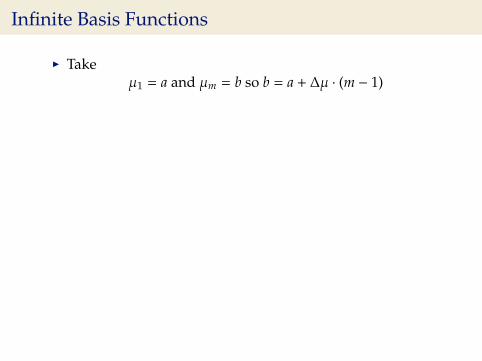
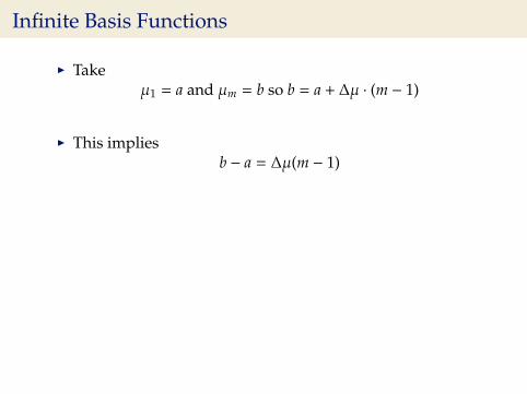
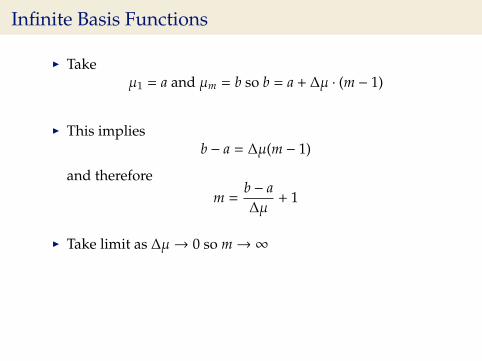
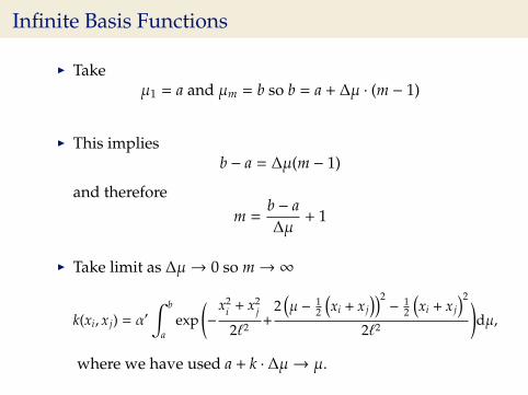
I Takeµ1 = a and µm = b so b = a + ∆µ · (m − 1)

I This impliesb − a = ∆µ(m − 1)

and thereforem =

b − a∆µ

+ 1

I Take limit as ∆µ→ 0 so m→∞

k(xi, x j) = α′∫ b

aexp

(−

x2i + x2

j

2`2 +2(µ − 1

2

(xi + x j

))2−

12

(xi + x j

)2

2`2

)dµ,

where we have used a + k · ∆µ→ µ.

Infinite Basis Functions

I Takeµ1 = a and µm = b so b = a + ∆µ · (m − 1)

I This impliesb − a = ∆µ(m − 1)

and thereforem =

b − a∆µ

+ 1

I Take limit as ∆µ→ 0 so m→∞

k(xi, x j) = α′∫ b

aexp

(−

x2i + x2

j

2`2 +2(µ − 1

2

(xi + x j

))2−

12

(xi + x j

)2

2`2

)dµ,

where we have used a + k · ∆µ→ µ.

Infinite Basis Functions

I Takeµ1 = a and µm = b so b = a + ∆µ · (m − 1)

I This impliesb − a = ∆µ(m − 1)

and thereforem =

b − a∆µ

+ 1

I Take limit as ∆µ→ 0 so m→∞

k(xi, x j) = α′∫ b

aexp

(−

x2i + x2

j

2`2 +2(µ − 1

2

(xi + x j

))2−

12

(xi + x j

)2

2`2

)dµ,

where we have used a + k · ∆µ→ µ.

Infinite Basis Functions

I Takeµ1 = a and µm = b so b = a + ∆µ · (m − 1)

I This impliesb − a = ∆µ(m − 1)

and thereforem =

b − a∆µ

+ 1

I Take limit as ∆µ→ 0 so m→∞

k(xi, x j) = α′∫ b

aexp

(−

x2i + x2

j

2`2 +2(µ − 1

2

(xi + x j

))2−

12

(xi + x j

)2

2`2

)dµ,

where we have used a + k · ∆µ→ µ.

Infinite Basis Functions

I Takeµ1 = a and µm = b so b = a + ∆µ · (m − 1)

I This impliesb − a = ∆µ(m − 1)

and thereforem =

b − a∆µ

+ 1

I Take limit as ∆µ→ 0 so m→∞

k(xi, x j) = α′∫ b

aexp

(−

x2i + x2

j

2`2 +2(µ − 1

2

(xi + x j

))2−

12

(xi + x j

)2

2`2

)dµ,

where we have used a + k · ∆µ→ µ.

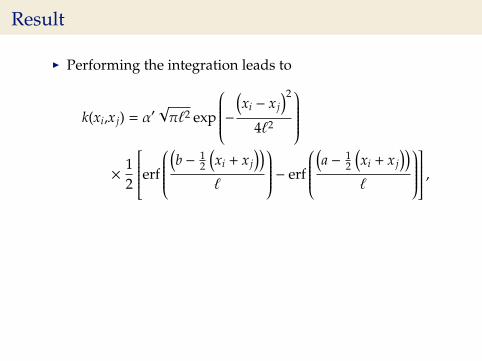
Result

I Performing the integration leads to

k(xi,x j) = α′√

π`2 exp

−(xi − x j

)2

4`2

×

12

erf

(b − 1

2

(xi + x j

))`

− erf

(a − 1

2

(xi + x j

))`

,

I Now take limit as a→ −∞ and b→∞

k(xi, x j

)= α exp

−(xi − x j

)2

4`2

.where α = α′

√

π`2.

Result

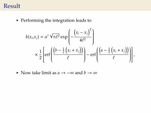
I Performing the integration leads to

k(xi,x j) = α′√

π`2 exp

−(xi − x j

)2

4`2

×

12

erf

(b − 1

2

(xi + x j

))`

− erf

(a − 1

2

(xi + x j

))`

,

I Now take limit as a→ −∞ and b→∞

k(xi, x j

)= α exp

−(xi − x j

)2

4`2

.where α = α′

√

π`2.

Result

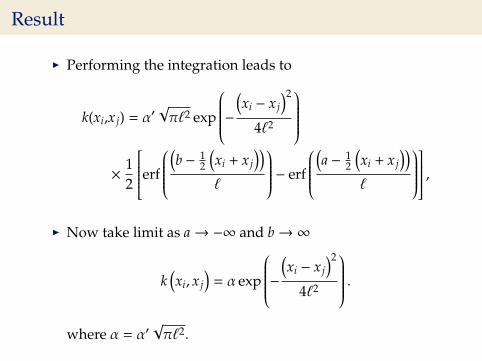
I Performing the integration leads to

k(xi,x j) = α′√

π`2 exp

−(xi − x j

)2

4`2

×

12

erf

(b − 1

2

(xi + x j

))`

− erf

(a − 1

2

(xi + x j

))`

,

I Now take limit as a→ −∞ and b→∞

k(xi, x j

)= α exp

−(xi − x j

)2

4`2

.where α = α′

√

π`2.

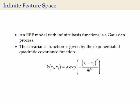
Infinite Feature Space

I An RBF model with infinite basis functions is a Gaussianprocess.

I The covariance function is given by the exponentiatedquadratic covariance function.

k(xi, x j

)= α exp

−(xi − x j

)2

4`2

.

Infinite Feature Space

I An RBF model with infinite basis functions is a Gaussianprocess.

I The covariance function is given by the exponentiatedquadratic covariance function.

k(xi, x j

)= α exp

−(xi − x j

)2

4`2

.

Infinite Feature Space

I An RBF model with infinite basis functions is a Gaussianprocess.

I The covariance function is the exponentiated quadratic.I Note: The functional form for the covariance function and

basis functions are similar.I this is a special case,I in general they are very different

Similar results can obtained for multi-dimensional inputmodels Williams (1998); Neal (1996).

Covariance FunctionsWhere did this covariance matrix come from?

Exponentiated Quadratic Kernel Function (RBF, SquaredExponential, Gaussian)

k (x, x′) = α exp

−‖x − x′‖222`2

I Covariance matrix is

built using the inputs tothe function x.

I For the example above itwas based on Euclideandistance.

I The covariance functionis also know as a kernel. ¡1¿ ¡2¿

Covariance Functions

RBF Basis Functions

k (x, x′) = αφ(x)>φ(x′)

φk(x) = exp

−∥∥∥x − µk

∥∥∥22

`2

µ =

−101

¡1¿ ¡2¿

-3-2-10123

-3 -2 -1 0 1 2 3

References I

P. S. Laplace. Essai philosophique sur les probabilites. Courcier, Paris, 2nd edition, 1814. Sixth edition of 1840 translatedand repreinted (1951) as A Philosophical Essay on Probabilities, New York: Dover; fifth edition of 1825 reprinted1986 with notes by Bernard Bru, Paris: Christian Bourgois Editeur, translated by Andrew Dale (1995) asPhilosophical Essay on Probabilities, New York:Springer-Verlag.

R. M. Neal. Bayesian Learning for Neural Networks. Springer, 1996. Lecture Notes in Statistics 118.

C. E. Rasmussen and C. K. I. Williams. Gaussian Processes for Machine Learning. MIT Press, Cambridge, MA, 2006.[Google Books] .

C. K. I. Williams. Computation with infinite neural networks. Neural Computation, 10(5):1203–1216, 1998.