Nearest Neighbour Searching in Metric Spaces

Kenneth Clarkson (1999, 2006)

Nearest Neighbour Search

Problem NN● Given:

– Set U– Distance measure D– Set of sites S ⊂ U– Query point q ∈ U

● Find:– Point p ∈ S such that D(p, q) is minimum

Outline● Applications and variations● Metric Spaces

– Basic inequalities

● Basic algorithms– Orchard, annulus, AESA, metric trees

● Dimensions– Coverings, packings, ε-nets

– Box, Hausdorff, packing, pointwise, doubling dimensions

– Estimating dimensions using NN

● NN using dimension bounds– Divide and conquer

● Exchangeable queries

– M(S, Q) and auxiliary query points

Applications

● “Post-office problem”– Given a location on a map, find the nearest post-

office/train station/restaurant...● Best-match file searching (key search)● Similarity search (databases)● Vector quantization (information theory)

– Find codeword that best approximates a message unit● Classification/clustering (pattern recognition)

– e.g. k-means clustering requires a nearest neighbour query for each point at each step

Variations

● k-nearest neighbours– Find k sites closest to query point q

● Distance range searching– Given query point q, distance r, find all sites p ∈ S s.t.

D(q, p) ≤ r● All (k) nearest neighbours

– For each site s, find its (k) nearest neighbour(s)● Closest pair

– Find sites s and s' s.t. D(s, s') is minimized over S

Variations

● Reverse queries– Return each site with q as its nearest neighbour in

S {∪ q} (excluding the site itself)● Approximate queries

– (δ)-nearest neighbour● Any point whose distance to q is within a δ factor of the

nearest neighbour distance– Interesting because approximate algorithms usually

achieve better running times than exact versions● Bichromatic queries

– Return closest red-blue pair

Metric Spaces

● Metric space Z := (U, D)– Set U– Distance measure D

● D satisfies1. Nonnegativity: D(x, y) ≥ 02. Small self-distance: D(x, x) = 03. Isolation: x ≠ y ⇒ D(x, y) > 04. Symmetry: D(x, y) = D(y, x)5. Triangle inequality: D(x, z) ≤ D(x, y) + D(y, z)

● Absence of any one of 3-5 can be “repaired”.

Triangle Inequality Bounds

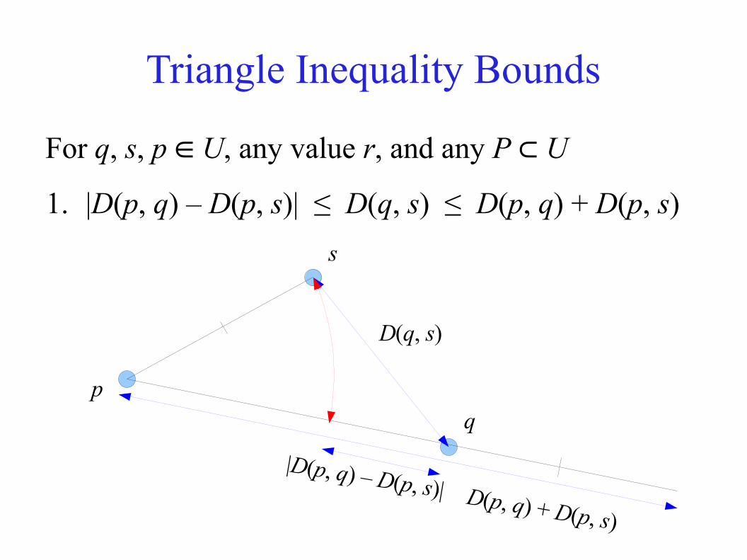
For q, s, p ∈ U, any value r, and any P ⊂ U

1. |D(p, q) – D(p, s)| ≤ D(q, s) ≤ D(p, q) + D(p, s)

pq

s

|D(p, q) – D(p, s)| D(p, q) + D(p, s)

D(q, s)

Triangle Inequality Bounds

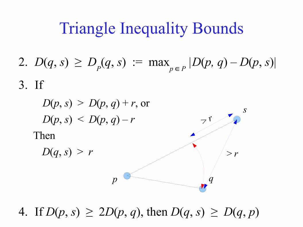
2. D(q, s) ≥ DP(q, s) := max

p ∈ P |D(p, q) – D(p, s)|

3. IfD(p, s) > D(p, q) + r, orD(p, s) < D(p, q) – r

ThenD(q, s) > r

4. If D(p, s) ≥ 2D(p, q), then D(q, s) ≥ D(q, p)

p q

s> r

> r

Triangle Inequality Bounds

● Utility: Give useful stopping criteria for NN searches

● Used by:– Orchard's Algorithm– Annulus Method– AESA– Metric Trees

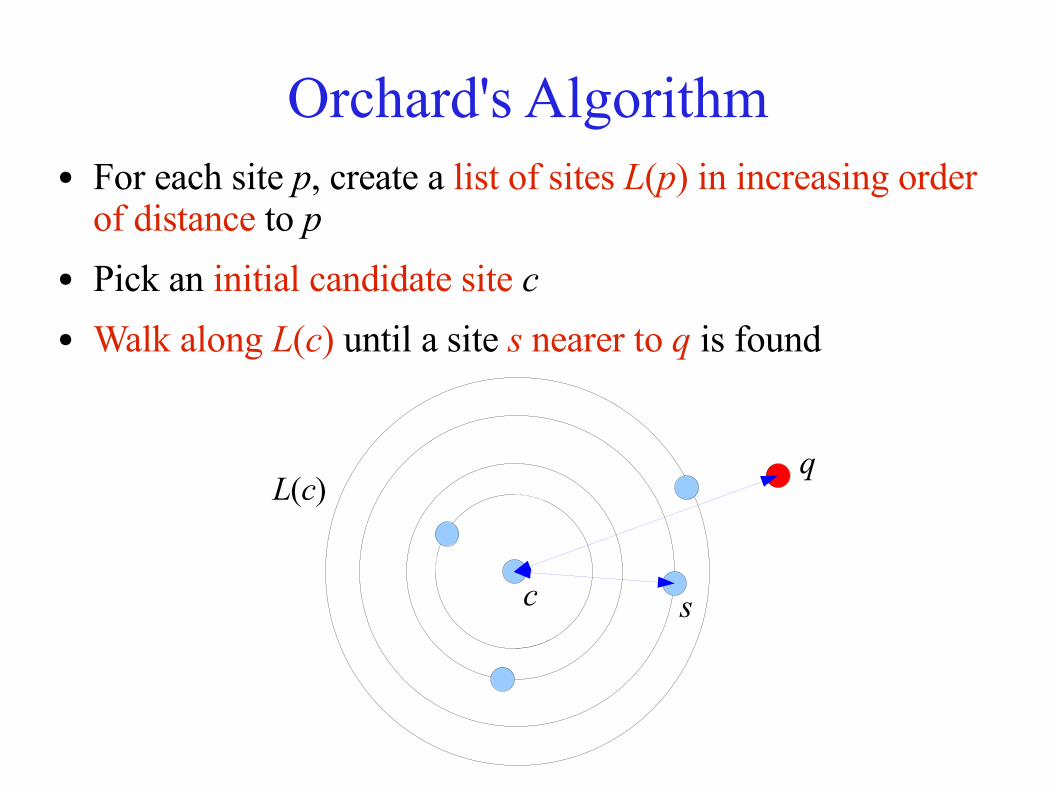
Orchard's Algorithm● For each site p, create a list of sites L(p) in increasing order

of distance to p● Pick an initial candidate site c● Walk along L(c) until a site s nearer to q is found

c s

qL(c)

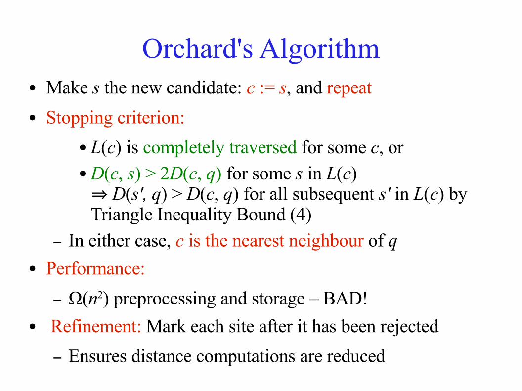
Orchard's Algorithm● Make s the new candidate: c := s, and repeat● Stopping criterion:

● L(c) is completely traversed for some c, or● D(c, s) > 2D(c, q) for some s in L(c)

⇒ D(s', q) > D(c, q) for all subsequent s' in L(c) by Triangle Inequality Bound (4)

– In either case, c is the nearest neighbour of q● Performance:

– Ω(n2) preprocessing and storage – BAD!● Refinement: Mark each site after it has been rejected

– Ensures distance computations are reduced

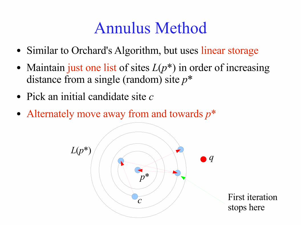
Annulus Method● Similar to Orchard's Algorithm, but uses linear storage● Maintain just one list of sites L(p*) in order of increasing

distance from a single (random) site p*● Pick an initial candidate site c● Alternately move away from and towards p*

p*

c

qL(p*)

First iteration stops here

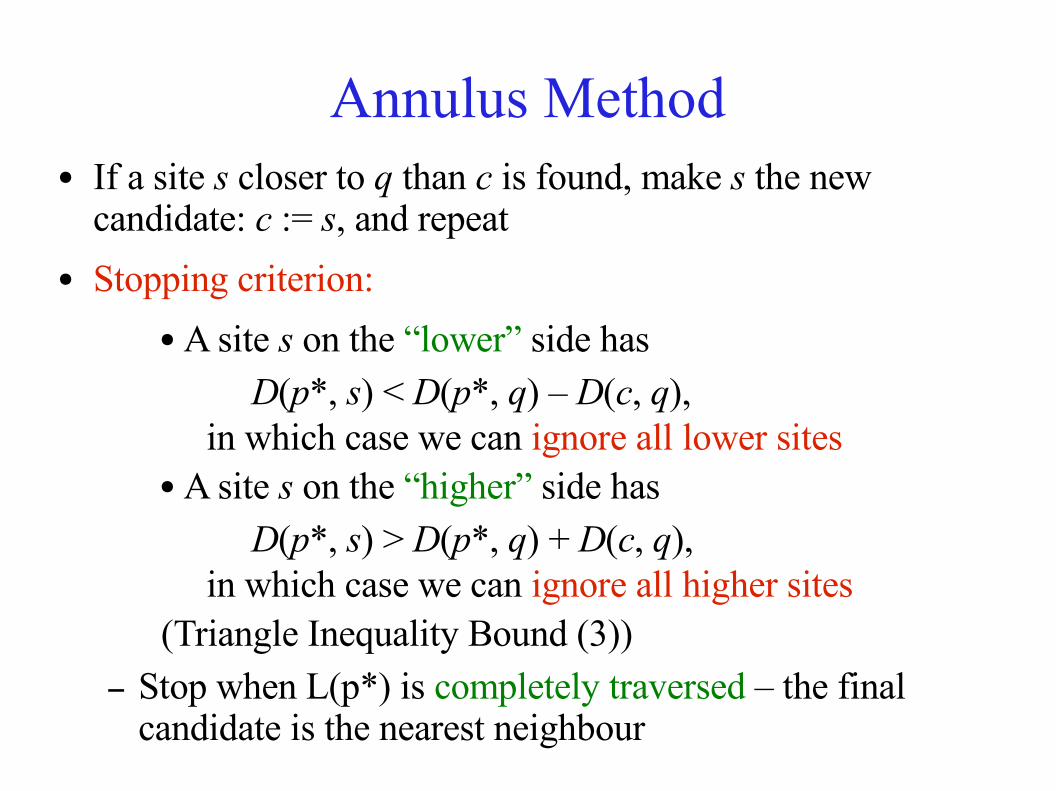
Annulus Method● If a site s closer to q than c is found, make s the new

candidate: c := s, and repeat● Stopping criterion:

● A site s on the “lower” side hasD(p*, s) < D(p*, q) – D(c, q),

in which case we can ignore all lower sites● A site s on the “higher” side has

D(p*, s) > D(p*, q) + D(c, q),in which case we can ignore all higher sites

(Triangle Inequality Bound (3))– Stop when L(p*) is completely traversed – the final

candidate is the nearest neighbour

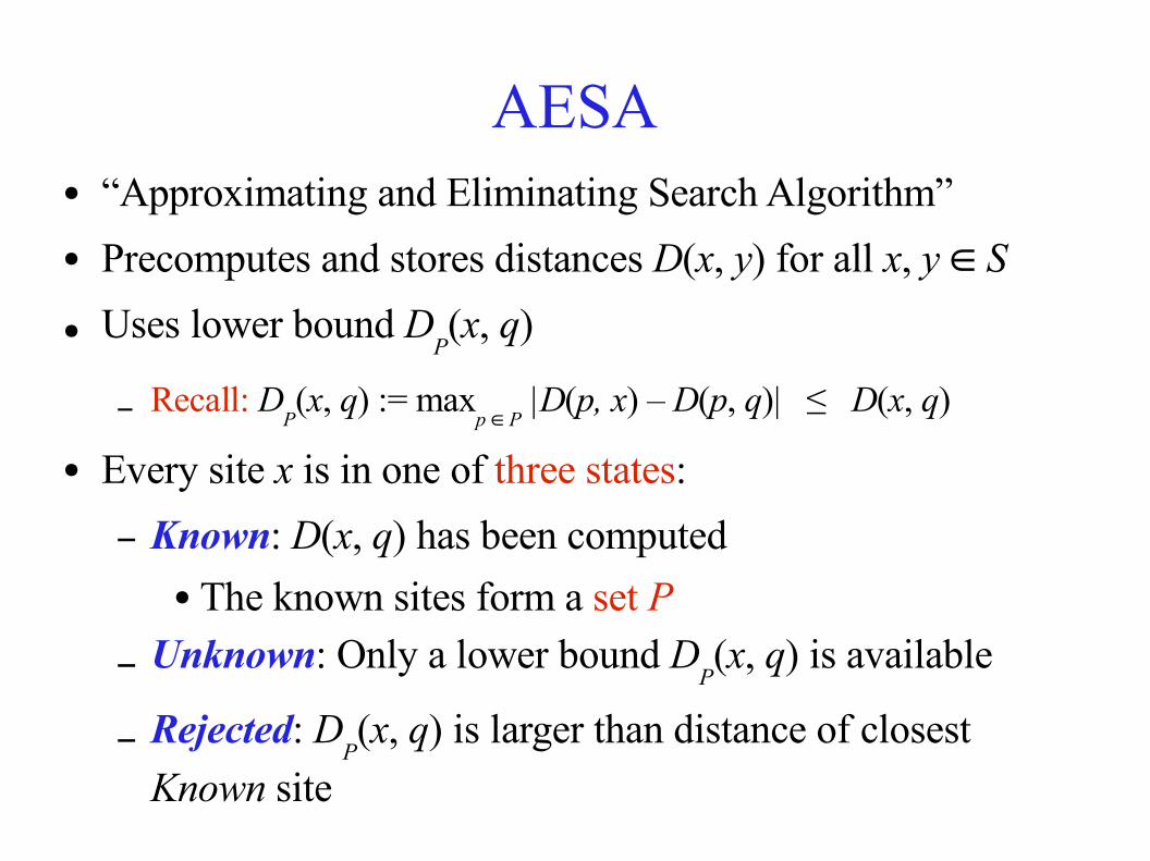
AESA● “Approximating and Eliminating Search Algorithm”● Precomputes and stores distances D(x, y) for all x, y ∈ S● Uses lower bound D

P(x, q)

– Recall: DP(x, q) := max

p ∈ P |D(p, x) – D(p, q)| ≤ D(x, q)

● Every site x is in one of three states:– Known: D(x, q) has been computed

● The known sites form a set P– Unknown: Only a lower bound D

P(x, q) is available

– Rejected: DP(x, q) is larger than distance of closest

Known site

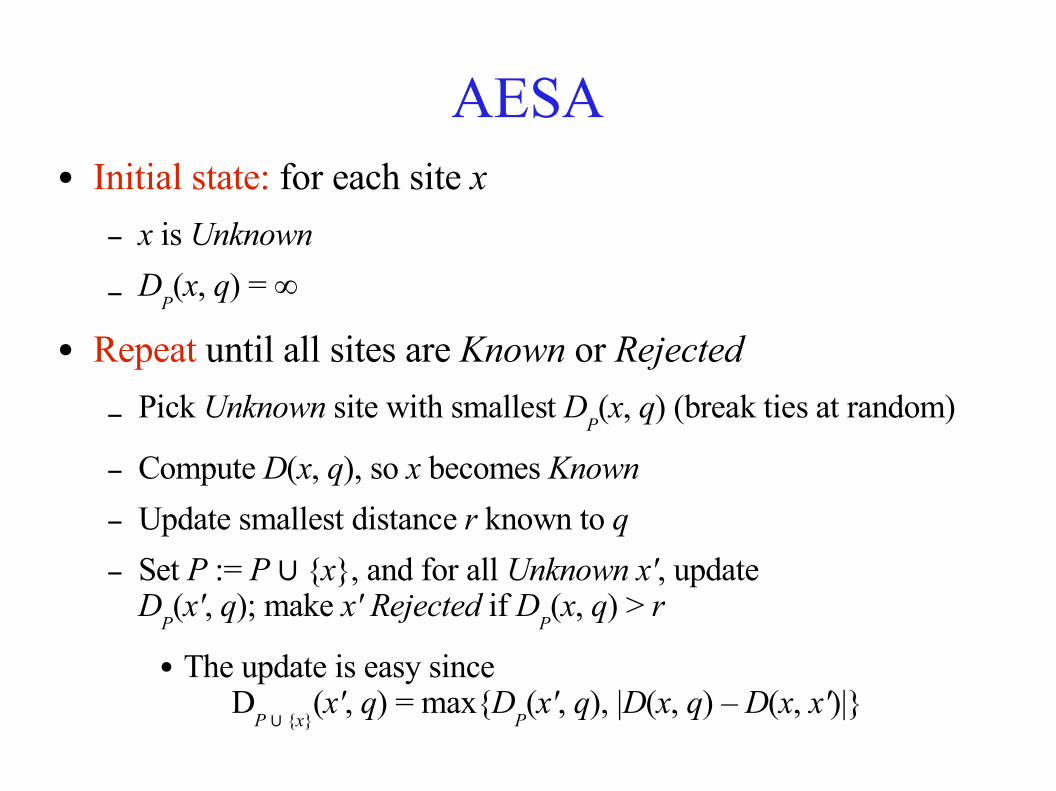
AESA● Initial state: for each site x

– x is Unknown

– DP(x, q) = ∞

● Repeat until all sites are Known or Rejected– Pick Unknown site with smallest D

P(x, q) (break ties at random)

– Compute D(x, q), so x becomes Known– Update smallest distance r known to q– Set P := P {∪ x}, and for all Unknown x', update

DP(x', q); make x' Rejected if D

P(x, q) > r

● The update is easy sinceD

P {∪ x}(x', q) = max{D

P(x', q), |D(x, q) – D(x, x')|}

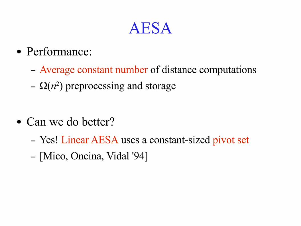
AESA● Performance:

– Average constant number of distance computations– Ω(n2) preprocessing and storage

● Can we do better?– Yes! Linear AESA uses a constant-sized pivot set– [Mico, Oncina, Vidal '94]

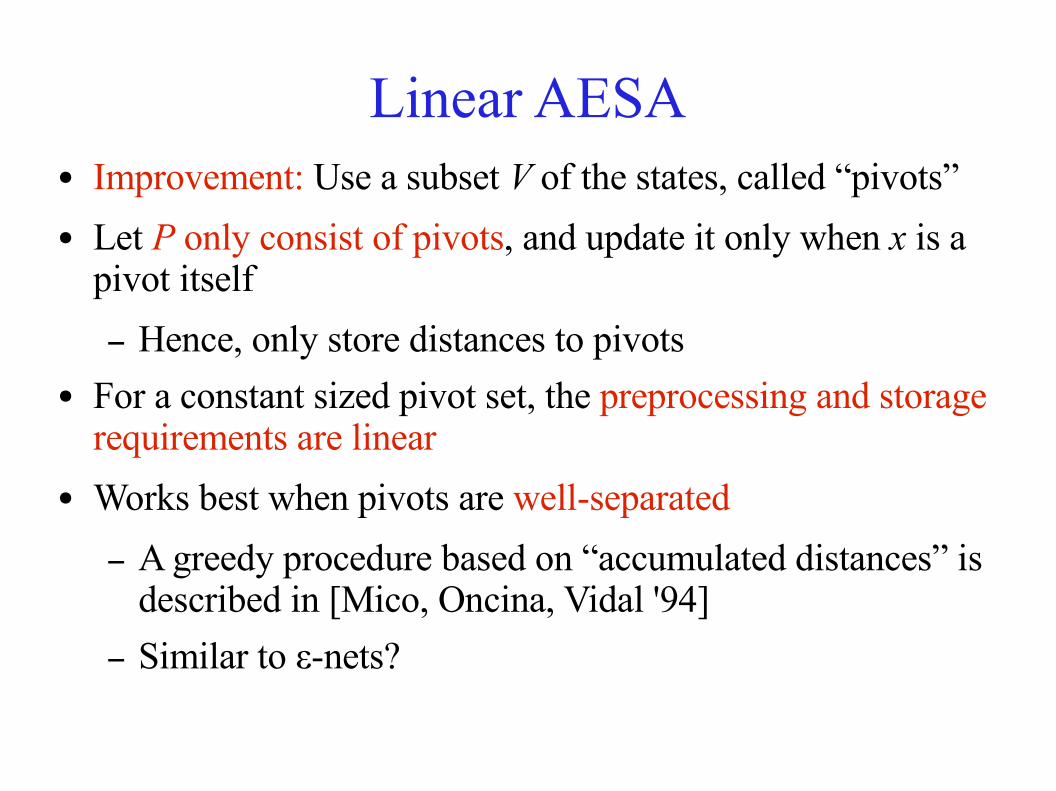
Linear AESA● Improvement: Use a subset V of the states, called “pivots”● Let P only consist of pivots, and update it only when x is a

pivot itself– Hence, only store distances to pivots

● For a constant sized pivot set, the preprocessing and storage requirements are linear

● Works best when pivots are well-separated– A greedy procedure based on “accumulated distances” is

described in [Mico, Oncina, Vidal '94]– Similar to ε-nets?

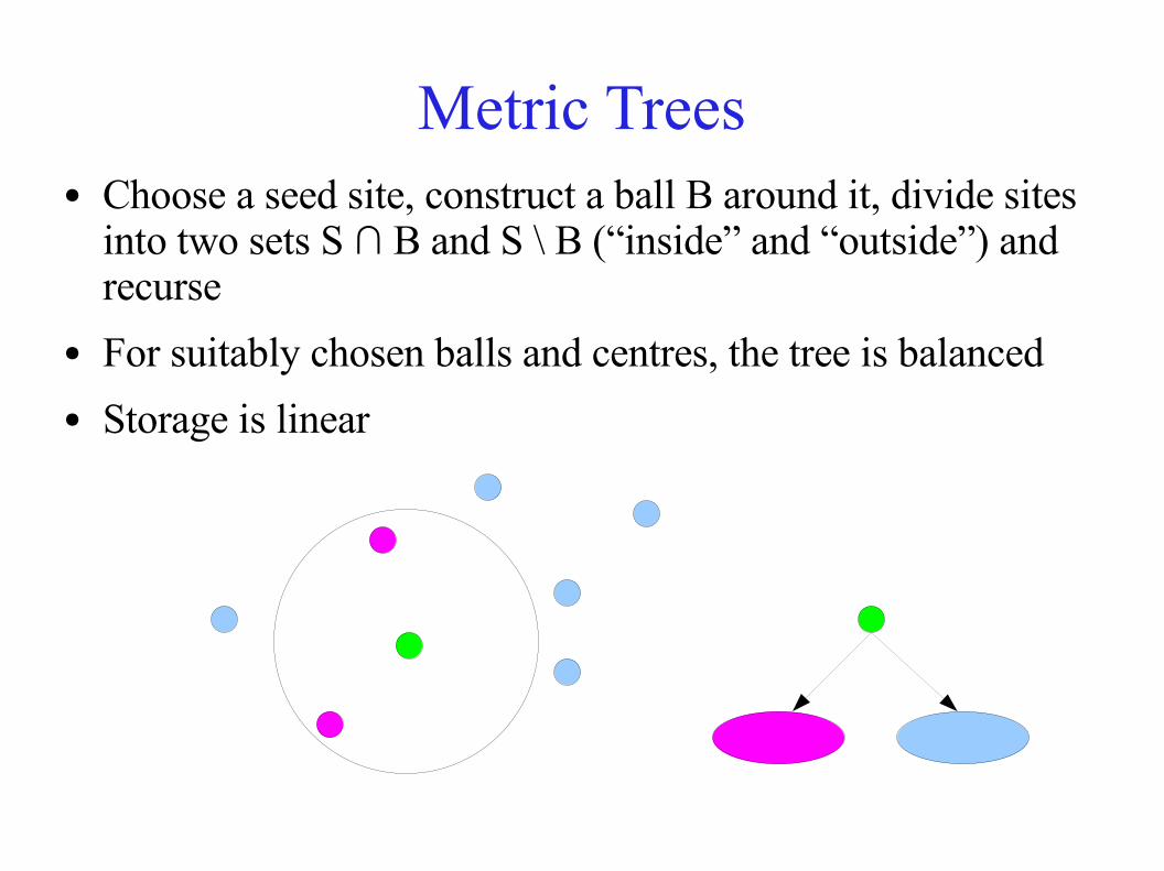
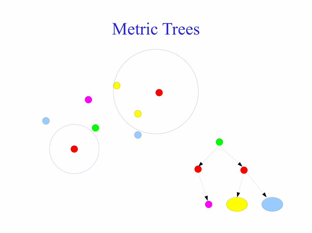
Metric Trees● Choose a seed site, construct a ball B around it, divide sites

into two sets S ∩ B and S \ B (“inside” and “outside”) and recurse

● For suitably chosen balls and centres, the tree is balanced● Storage is linear

Metric Trees

Metric Trees

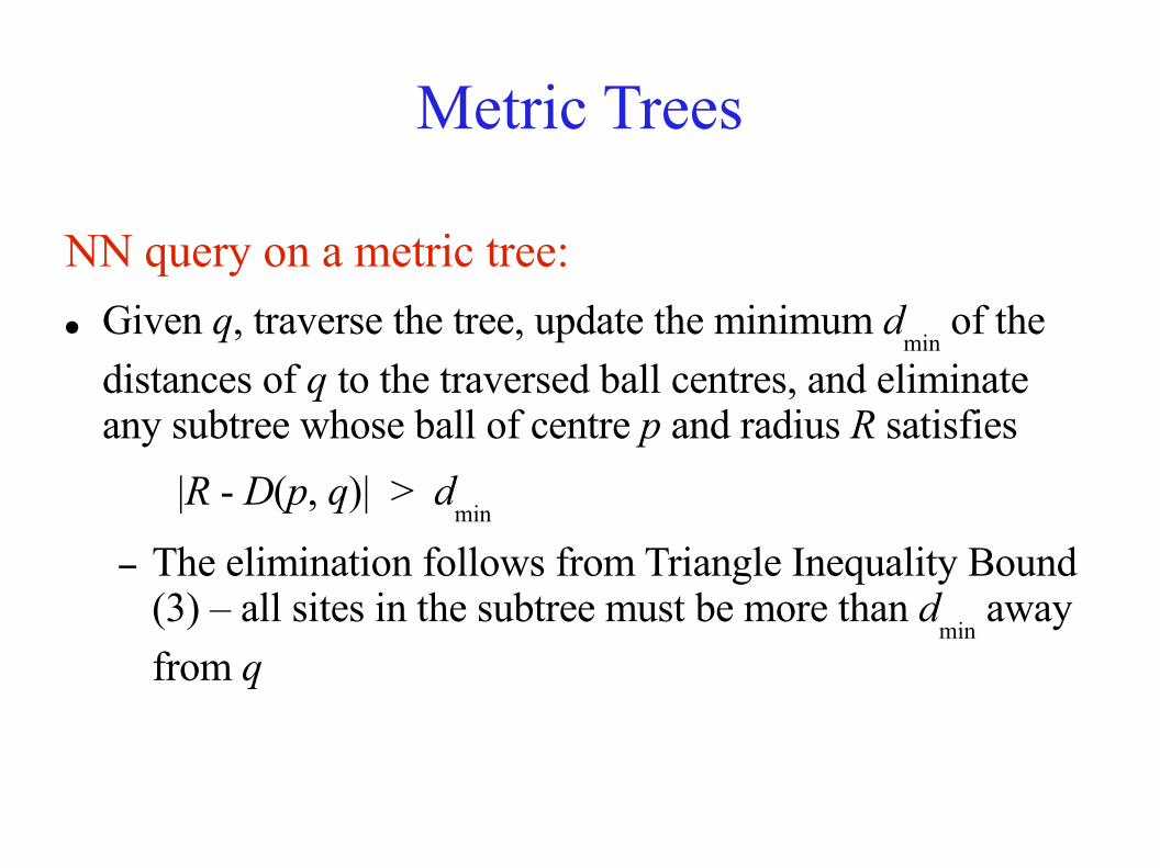
NN query on a metric tree:● Given q, traverse the tree, update the minimum d

min of the

distances of q to the traversed ball centres, and eliminate any subtree whose ball of centre p and radius R satisfies

|R - D(p, q)| > dmin

– The elimination follows from Triangle Inequality Bound (3) – all sites in the subtree must be more than d

min away

from q

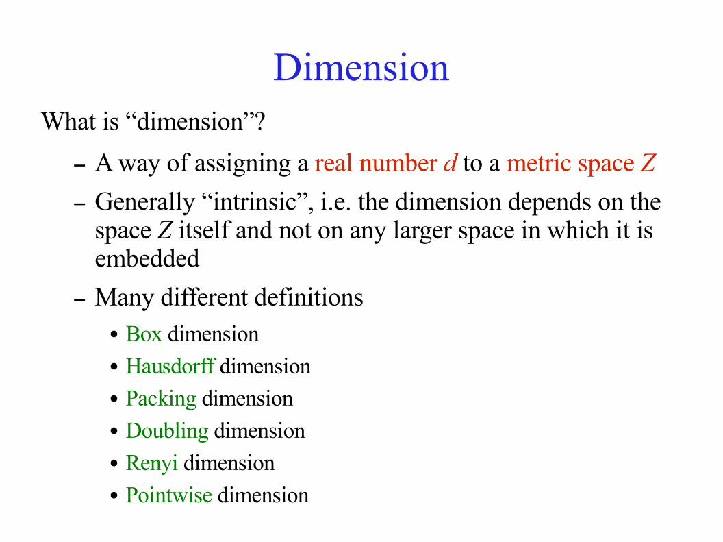
DimensionWhat is “dimension”?

– A way of assigning a real number d to a metric space Z– Generally “intrinsic”, i.e. the dimension depends on the

space Z itself and not on any larger space in which it is embedded

– Many different definitions● Box dimension● Hausdorff dimension● Packing dimension● Doubling dimension● Renyi dimension● Pointwise dimension

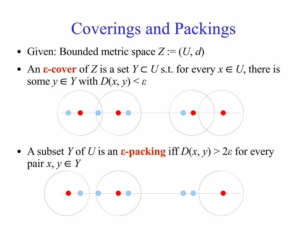
Coverings and Packings● Given: Bounded metric space Z := (U, d)● An ε-cover of Z is a set Y ⊂ U s.t. for every x ∈ U, there is

some y ∈ Y with D(x, y) < ε

● A subset Y of U is an ε-packing iff D(x, y) > 2ε for every pair x, y ∈ Y

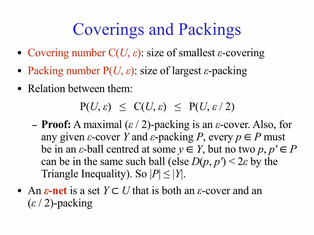
Coverings and Packings● Covering number C(U, ε): size of smallest ε-covering● Packing number P(U, ε): size of largest ε-packing● Relation between them:

P(U, ε) ≤ C(U, ε) ≤ P(U, ε / 2)– Proof: A maximal (ε / 2)-packing is an ε-cover. Also, for

any given ε-cover Y and ε-packing P, every p ∈ P must be in an ε-ball centred at some y ∈ Y, but no two p, p' ∈ P can be in the same such ball (else D(p, p') < 2ε by the Triangle Inequality). So |P| ≤ |Y|.

● An ε-net is a set Y ⊂ U that is both an ε-cover and an(ε / 2)-packing

Various Dimensions

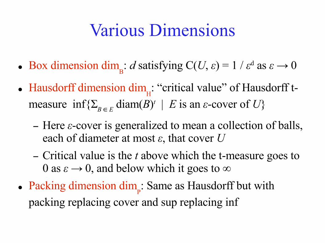
● Box dimension dimB: d satisfying C(U, ε) = 1 / εd as ε → 0

● Hausdorff dimension dimH: “critical value” of Hausdorff t-

measure inf{ΣB ∈ E diam(B)t | E is an ε-cover of U}

– Here ε-cover is generalized to mean a collection of balls, each of diameter at most ε, that cover U

– Critical value is the t above which the t-measure goes to 0 as ε → 0, and below which it goes to ∞

● Packing dimension dimP: Same as Hausdorff but with

packing replacing cover and sup replacing inf

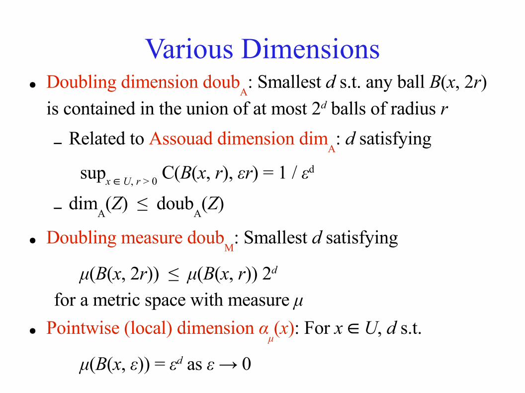
Various Dimensions● Doubling dimension doub

A: Smallest d s.t. any ball B(x, 2r)

is contained in the union of at most 2d balls of radius r

– Related to Assouad dimension dimA: d satisfying

supx ∈ U, r > 0 C(B(x, r), εr) = 1 / εd

– dimA(Z) ≤ doub

A(Z)

● Doubling measure doubM

: Smallest d satisfying

µ(B(x, 2r)) ≤ µ(B(x, r)) 2d

for a metric space with measure µ● Pointwise (local) dimension α

µ(x): For x ∈ U, d s.t.

µ(B(x, ε)) = εd as ε → 0

Dimension Estimation using NN:An Example

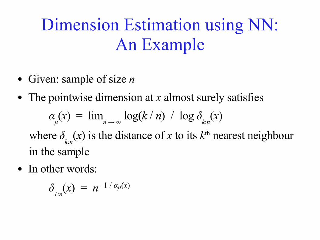
● Given: sample of size n● The pointwise dimension at x almost surely satisfies

αµ(x) = lim

n → ∞ log(k / n) / log δ

k:n(x)

where δk:n

(x) is the distance of x to its kth nearest neighbour in the sample

● In other words:

δ1:n

(x) = n -1 / αµ(x)

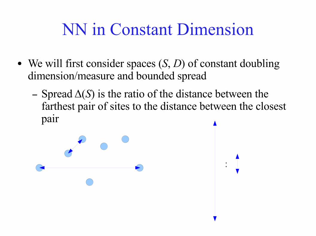
NN in Constant Dimension

● We will first consider spaces (S, D) of constant doubling dimension/measure and bounded spread– Spread Δ(S) is the ratio of the distance between the

farthest pair of sites to the distance between the closest pair

:

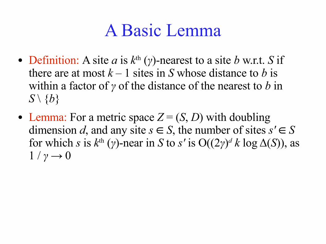
A Basic Lemma● Definition: A site a is kth (γ)-nearest to a site b w.r.t. S if

there are at most k – 1 sites in S whose distance to b is within a factor of γ of the distance of the nearest to b inS \ {b}

● Lemma: For a metric space Z = (S, D) with doubling dimension d, and any site s ∈ S, the number of sites s' ∈ S for which s is kth (γ)-near in S to s' is O((2γ)d k log Δ(S)), as 1 / γ → 0

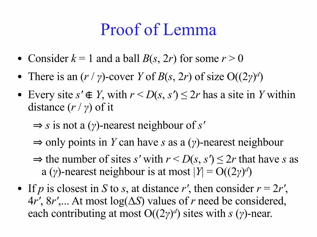
Proof of Lemma● Consider k = 1 and a ball B(s, 2r) for some r > 0● There is an (r / γ)-cover Y of B(s, 2r) of size O((2γ)d)● Every site s' ∉ Y, with r < D(s, s') ≤ 2r has a site in Y within

distance (r / γ) of it ⇒ s is not a (γ)-nearest neighbour of s' ⇒ only points in Y can have s as a (γ)-nearest neighbour ⇒ the number of sites s' with r < D(s, s') ≤ 2r that have s as a (γ)-nearest neighbour is at most |Y| = O((2γ)d)

● If p is closest in S to s, at distance r', then consider r = 2r', 4r', 8r',... At most log(ΔS) values of r need be considered, each contributing at most O((2γ)d) sites with s (γ)-near.

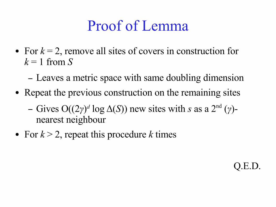
Proof of Lemma● For k = 2, remove all sites of covers in construction for

k = 1 from S– Leaves a metric space with same doubling dimension

● Repeat the previous construction on the remaining sites– Gives O((2γ)d log Δ(S)) new sites with s as a 2nd (γ)-

nearest neighbour● For k > 2, repeat this procedure k times

Q.E.D.

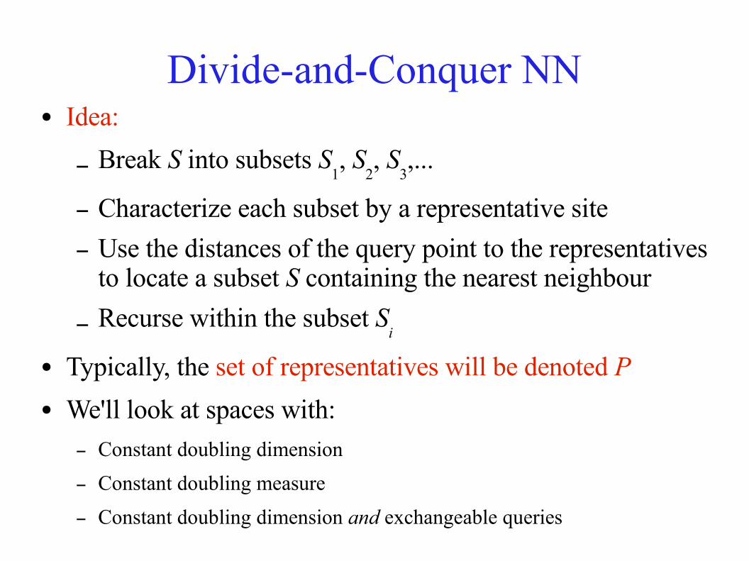
Divide-and-Conquer NN● Idea:

– Break S into subsets S1, S

2, S

3,...

– Characterize each subset by a representative site– Use the distances of the query point to the representatives

to locate a subset S containing the nearest neighbour– Recurse within the subset S

i

● Typically, the set of representatives will be denoted P● We'll look at spaces with:

– Constant doubling dimension– Constant doubling measure– Constant doubling dimension and exchangeable queries

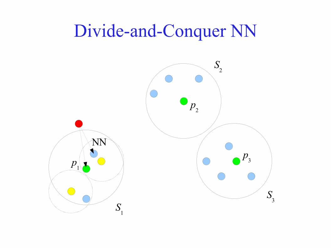
Divide-and-Conquer NN

NN

p1

p2

p3

S1

S2

S3

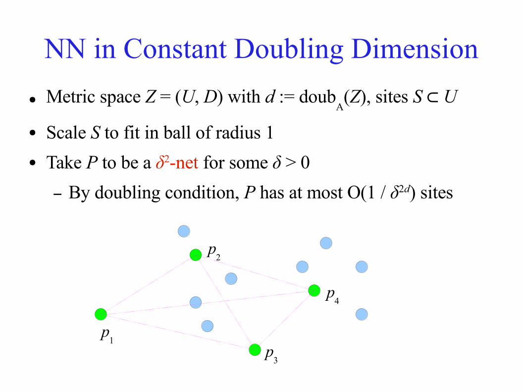
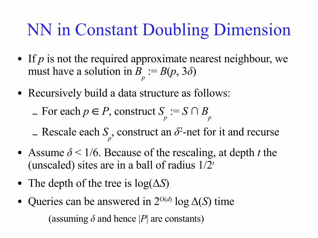
NN in Constant Doubling Dimension● Metric space Z = (U, D) with d := doub

A(Z), sites S ⊂ U

● Scale S to fit in ball of radius 1● Take P to be a δ2-net for some δ > 0

– By doubling condition, P has at most O(1 / δ2d) sites

p1

p2

p3

p4

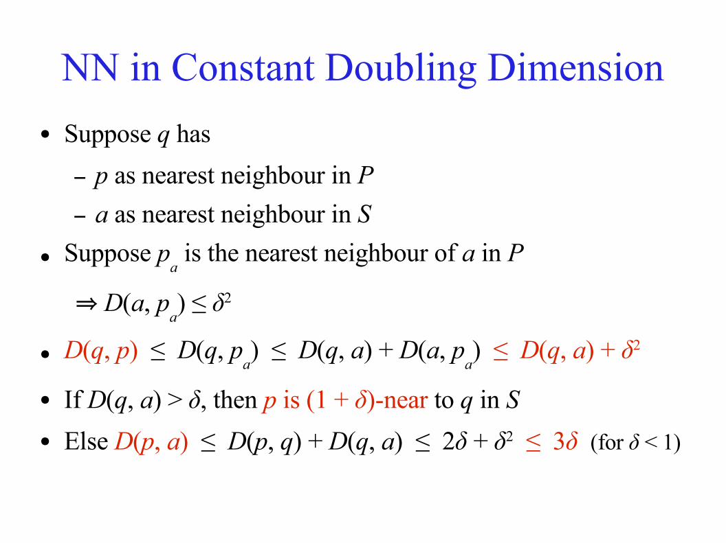
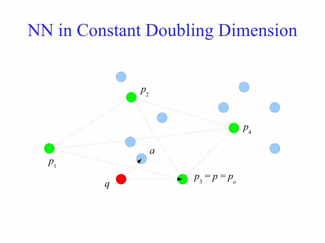
NN in Constant Doubling Dimension● Suppose q has

– p as nearest neighbour in P– a as nearest neighbour in S

● Suppose pa is the nearest neighbour of a in P

⇒ D(a, pa) ≤ δ2

● D(q, p) ≤ D(q, pa) ≤ D(q, a) + D(a, p

a) ≤ D(q, a) + δ2

● If D(q, a) > δ, then p is (1 + δ)-near to q in S● Else D(p, a) ≤ D(p, q) + D(q, a) ≤ 2δ + δ2 ≤ 3δ (for δ < 1)

NN in Constant Doubling Dimension

p1

p2

p3 = p = p

a

p4

q

a

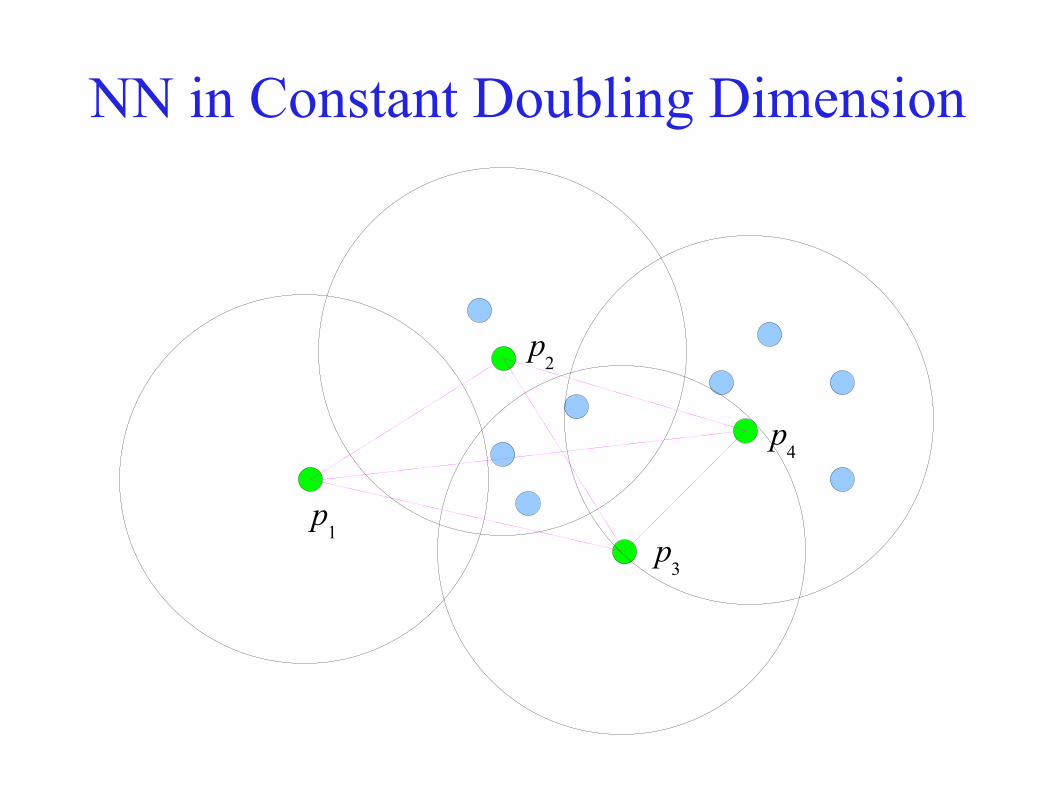
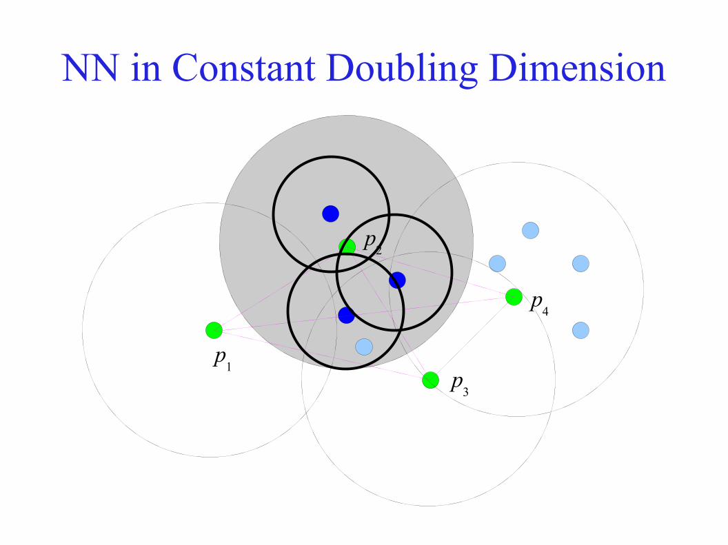
NN in Constant Doubling Dimension● If p is not the required approximate nearest neighbour, we

must have a solution in Bp := B(p, 3δ)

● Recursively build a data structure as follows:

– For each p ∈ P, construct Sp := S ∩ B

p

– Rescale each Sp, construct an δ2-net for it and recurse

● Assume δ < 1/6. Because of the rescaling, at depth t the (unscaled) sites are in a ball of radius 1/2t

● The depth of the tree is log(ΔS)● Queries can be answered in 2O(d) log Δ(S) time

(assuming δ and hence |P| are constants)

NN in Constant Doubling Dimension

p1

p2

p3

p4

NN in Constant Doubling Dimension

p1

p2

p3

p4

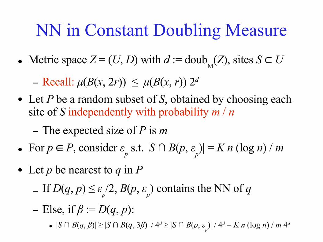
NN in Constant Doubling Measure● Metric space Z = (U, D) with d := doub

M(Z), sites S ⊂ U

– Recall: µ(B(x, 2r)) ≤ µ(B(x, r)) 2d

● Let P be a random subset of S, obtained by choosing each site of S independently with probability m / n– The expected size of P is m

● For p ∈ P, consider εp s.t. |S ∩ B(p, ε

p)| = K n (log n) / m

● Let p be nearest to q in P

– If D(q, p) ≤ εp/2, B(p, ε

p) contains the NN of q

– Else, if β := D(q, p):● |S ∩ B(q, β)| ≥ |S ∩ B(q, 3β)| / 4d ≥ |S ∩ B(p, ε

p)| / 4d = K n (log n) / m 4d

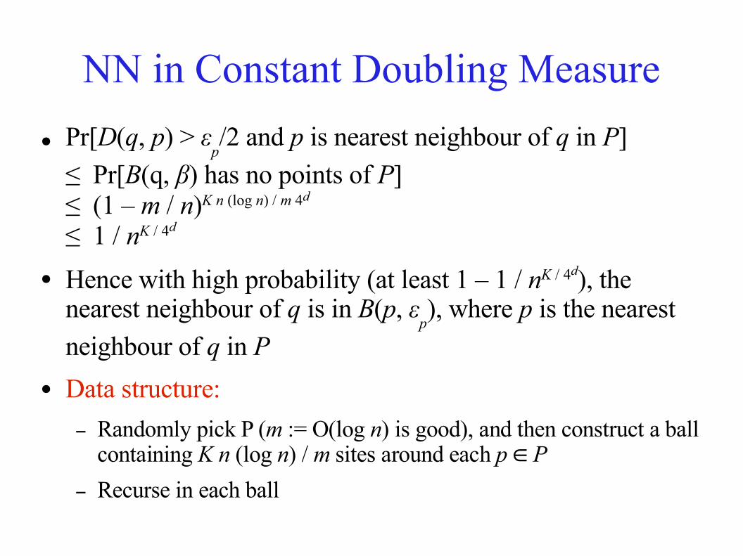
NN in Constant Doubling Measure● Pr[D(q, p) > ε

p/2 and p is nearest neighbour of q in P]

≤ Pr[B(q, β) has no points of P]≤ (1 – m / n)K n (log n) / m 4d

≤ 1 / nK / 4d

● Hence with high probability (at least 1 – 1 / nK / 4d), the nearest neighbour of q is in B(p, ε

p), where p is the nearest

neighbour of q in P● Data structure:

– Randomly pick P (m := O(log n) is good), and then construct a ball containing K n (log n) / m sites around each p ∈ P

– Recurse in each ball

NN in Constant Doubling Dimension with Exchangeable Queries

We have an approximation algorithm for constant doubling dimension and an exact algorithm (with some prob. of error) for constant doubling measure

– But the former seems more robust than the latter– Is there an exact algorithm?– Yes! If we assume “exchangeability”:

● Sites and queries drawn from same distribution– Use the usual divide-and-conquer method, using the

results of the next slide to construct subsets at each step

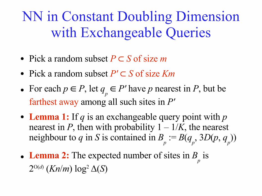
NN in Constant Doubling Dimension with Exchangeable Queries

● Pick a random subset P ⊂ S of size m● Pick a random subset P' ⊂ S of size Km● For each p ∈ P, let q

p ∈ P' have p nearest in P, but be

farthest away among all such sites in P'● Lemma 1: If q is an exchangeable query point with p

nearest in P, then with probability 1 – 1/K, the nearest neighbour to q in S is contained in B

p := B(q

p, 3D(p, q

p))

● Lemma 2: The expected number of sites in Bp is

2O(d) (Kn/m) log2 Δ(S)

M(S, Q)

● [Clarkson '99]● A skiplist-type data structure for NN● Requires auxiliary set Q of m points● Achieves:

– Near-linear preprocessing and storage– Sublinear query time

● Analysis requires:– Exchangeability of q, Q and S

● Q is “typical set of queries”

M(S, Q)● Definition:

– p ∈ S is a (γ)-nearest neighbour of q w.r.t. R ⊂ S ifD(p, q) ≤ γD(q, R)

– Denote this by q →γ p or p γ← q● Pick γ, and construct M(S, Q) as follows:

– Let (p1, p

2,..., p

n) be a random permutation of S

– Let Ri := {p

1, p

2,..., p

i}

– Similarly shuffle Q● Q

j is a random subset of Q of size j

● Define Qj := Q for j > m

M(S, Q)● Define A

j as:

{pi | i > j, ∃ q ∈ Q

Ki with p

j 1← q →γ p

i, w.r.t. Ri – 1}

● pj is the nearest neighbour of q in R

i-1

● D(q, pi) ≤ γD(q, p

j)

● Construction can be done by adding random points (without repetition) from S one at a time to construct R

i from R

i-1, and

updating Aj's at each step

● The sites in Aj are in increasing order of index i

● Searching is exactly the same as for Orchard's Algorithm, with p

1 the initial candidate

M(S, Q): Failure Probability● Assume Q and q are exchangeable and

Kn < m = nO(1). If γ = 3, the probability that M(S, Q) fails to return a nearest site to q in S is O(log2 n) / K– Holds in any metric space

● For general γ: Suppose Z := (U, D) has a “γ-dominator bound”. Under the same conditions as above, but for general γ, the failure probability is O(D

γ log2 n) / K

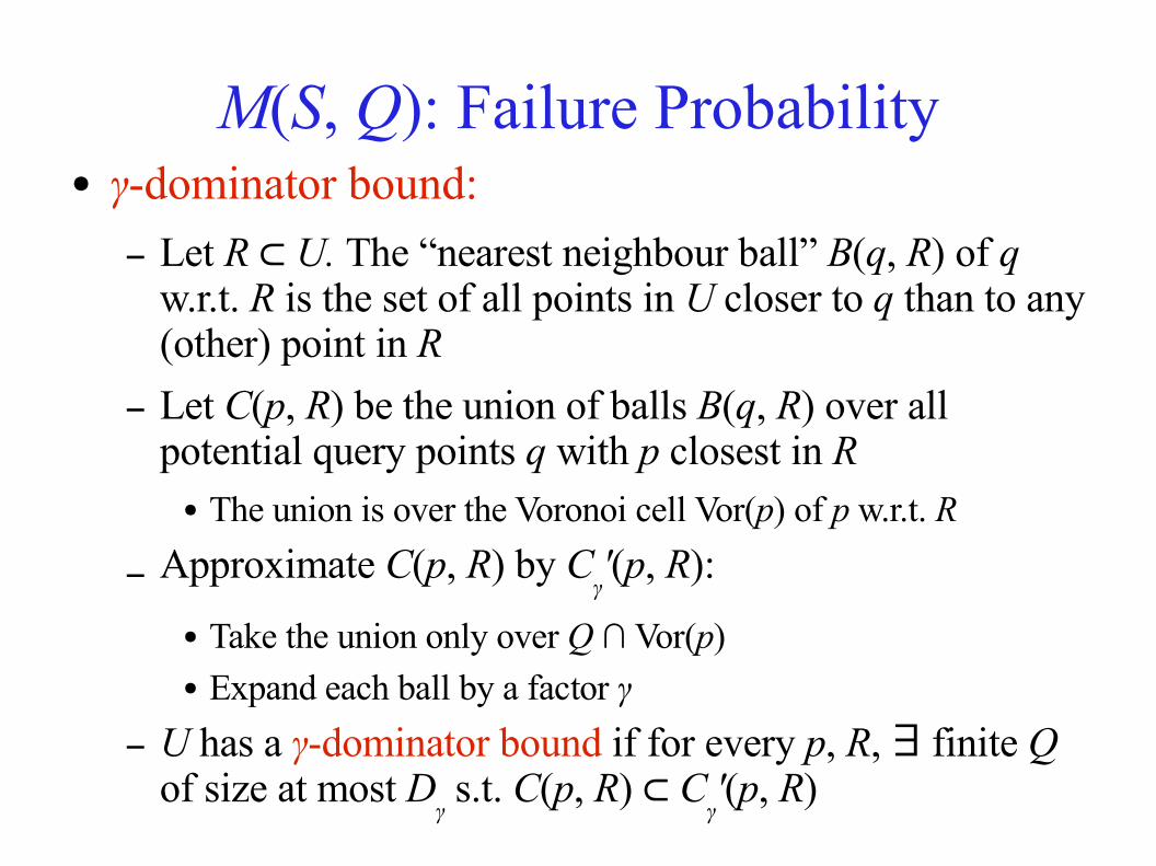
M(S, Q): Failure Probability● γ-dominator bound:

– Let R ⊂ U. The “nearest neighbour ball” B(q, R) of q w.r.t. R is the set of all points in U closer to q than to any (other) point in R

– Let C(p, R) be the union of balls B(q, R) over all potential query points q with p closest in R

● The union is over the Voronoi cell Vor(p) of p w.r.t. R

– Approximate C(p, R) by Cγ'(p, R):

● Take the union only over Q ∩ Vor(p)● Expand each ball by a factor γ

– U has a γ-dominator bound if for every p, R, finite ∃ Q of size at most D

γ s.t. C(p, R) ⊂ C

γ'(p, R)

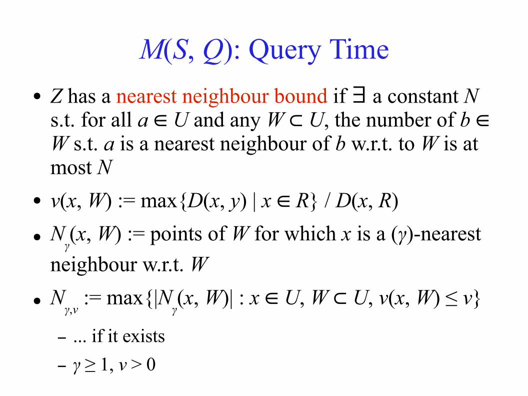
M(S, Q): Query Time● Z has a nearest neighbour bound if a constant ∃ N

s.t. for all a ∈ U and any W ⊂ U, the number of b ∈W s.t. a is a nearest neighbour of b w.r.t. to W is at most N

● v(x, W) := max{D(x, y) | x ∈ R} / D(x, R)● N

γ(x, W) := points of W for which x is a (γ)-nearest

neighbour w.r.t. W● N

γ,v := max{|N

γ(x, W)| : x ∈ U, W ⊂ U, v(x, W) ≤ v}

– ... if it exists– γ ≥ 1, v > 0

M(S, Q): Query Time

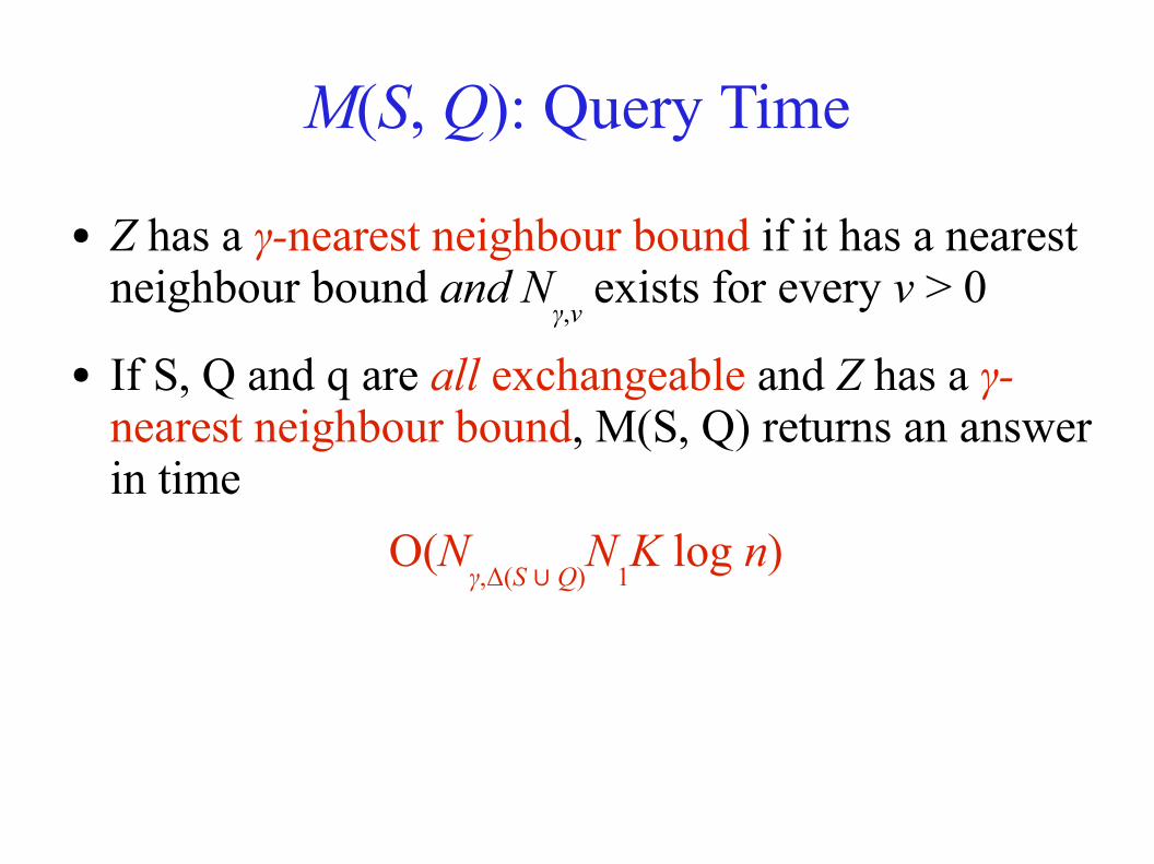
● Z has a γ-nearest neighbour bound if it has a nearest neighbour bound and N

γ,v exists for every v > 0

● If S, Q and q are all exchangeable and Z has a γ-nearest neighbour bound, M(S, Q) returns an answer in time

O(Nγ,Δ(S ∪ Q)

N1K log n)

M(S, Q): Storage

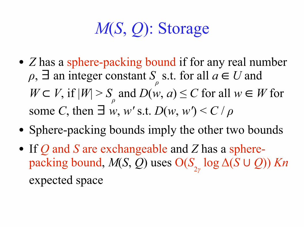
● Z has a sphere-packing bound if for any real number ρ, an integer constant ∃ S

ρ s.t. for all a ∈ U and

W ⊂ V, if |W| > Sρ and D(w, a) ≤ C for all w ∈W for

some C, then ∃ w, w' s.t. D(w, w') < C / ρ● Sphere-packing bounds imply the other two bounds● If Q and S are exchangeable and Z has a sphere-

packing bound, M(S, Q) uses O(S2γ

log Δ(S ∪ Q)) Kn expected space