Natural Sciences Tripos Part IB

Mathematical Methods I

Michaelmas 2014

Dr Henrik Latter

i

2

Schedule

Vector calculus. Suffix notation. Contractions using δij and ϵijk. Re-

minder of vector products, grad, div, curl, ∇2 and their representations

using suffix notation. Divergence theorem and Stokes’s theorem. Vector

differential operators in orthogonal curvilinear coordinates, e.g. cylindrical

and spherical polar coordinates. Jacobians. [6 lectures]

Partial differential equations. Linear second-order partial differential

equations; physical examples of occurrence, the method of separation of

variables (Cartesian coordinates only). [2]

Green’s functions. Response to impulses, delta function (treated heuris-

tically), Green’s functions for initial and boundary value problems. [3]

Fourier transform. Fourier transforms; relation to Fourier series, sim-

ple properties and examples, convolution theorem, correlation fnuctions,

Parseval’s theorem and power spectra. [2]

Matrices. N -dimensional vector spaces, matrices, scalar product, trans-

formation of basis vectors. Eigenvalues and eigenvectors of a matrix; de-

generate case, stationary property of eigenvalues. Orthogonal and unitary

transformations. Quadratic & Hermitian forms, quadric surfaces. [5]

Elementary analysis. Idea of convergence and limits. O notation.

Statement of Taylor’s theorem with discussion of remainder. Convergence

of series; comparison and ratio tests. Power series of a complex variable;

circle of convergence. Analytic functions: Cauchy–Riemann equations,

rational functions and exp(z). Zeros, poles and essential singularities. [3]

Series solutions of ordinary differential equations. Homogeneous

equations; solution by series (without full discussion of logarithmic sin-

gularities), exemplified by Legendre’s equation. Classification of singular

points. Indicial equations and local behaviour of solutions near singular

points. [3]

3

Course websites

camtools.cam.ac.uk Maths : NSTIB 14 15

www.damtp.cam.ac.uk/user/hl278/NST

Assumed knowledge

I will assume familiarity with the following topics at the level of Course A

of Part IA Mathematics for Natural Sciences.

• Algebra of complex numbers

• Algebra of vectors (including scalar and vector products)

• Algebra of matrices

• Eigenvalues and eigenvectors of matrices

• Taylor series and the geometric series

• Calculus of functions of several variables

• Line, surface and volume integrals

• The Gaussian integral

• First-order ordinary differential equations

• Second-order linear ODEs with constant coefficients

• Fourier series

4

Textbooks

The following textbooks are recommended. The first grew out of the NST

Maths course, so it will be particularly close to the lectures in places.

• K. F. Riley, M. P. Hobson and S. J. Bence (2006). Mathematical

Methods for Physics and Engineering, 3rd edition. Cambridge Univer-

sity Press

• G. Arfken and H. J. Weber (2005). Mathematical Methods for Physi-

cists, 6th edition. Academic Press

Questions

• Please ask questions in lecture, especially brief ones (typos, jargon)

• Longer questions can be e-mailed to me: hl278@cam.ac.uk. Turnaround

time: approximately 1-3 days

1 VECTOR CALCULUS 1

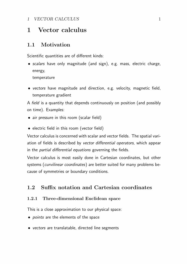
1 Vector calculus

1.1 Motivation

Scientific quantities are of different kinds:

• scalars have only magnitude (and sign), e.g. mass, electric charge,

energy,

temperature

• vectors have magnitude and direction, e.g. velocity, magnetic field,

temperature gradient

A field is a quantity that depends continuously on position (and possibly

on time). Examples:

• air pressure in this room (scalar field)

• electric field in this room (vector field)

Vector calculus is concerned with scalar and vector fields. The spatial vari-

ation of fields is described by vector differential operators, which appear

in the partial differential equations governing the fields.

Vector calculus is most easily done in Cartesian coordinates, but other

systems (curvilinear coordinates) are better suited for many problems be-

cause of symmetries or boundary conditions.

1.2 Suffix notation and Cartesian coordinates

1.2.1 Three-dimensional Euclidean space

This is a close approximation to our physical space:

• points are the elements of the space

• vectors are translatable, directed line segments

1 VECTOR CALCULUS 2

• Euclidean means that lengths and angles obey the classical results of

geometry

Points and vectors have a geometrical existence without reference to any

coordinate system. For definite calculations, however, we must introduce

coordinates.

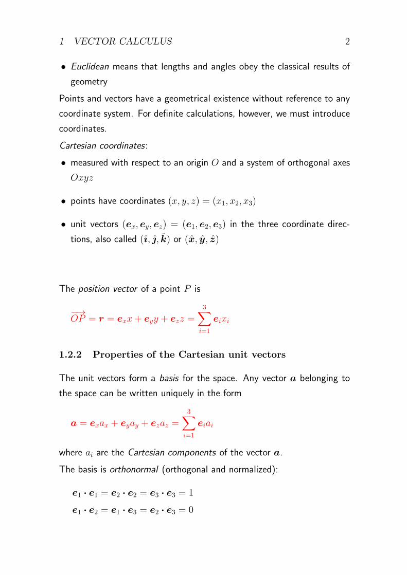
Cartesian coordinates:

• measured with respect to an origin O and a system of orthogonal axes

Oxyz

• points have coordinates (x, y, z) = (x1, x2, x3)

• unit vectors (ex, ey, ez) = (e1, e2, e3) in the three coordinate direc-

tions, also called (ı, ȷ, k) or (x, y, z)

The position vector of a point P is

−→OP = r = exx+ eyy + ezz =

3∑i=1

eixi

1.2.2 Properties of the Cartesian unit vectors

The unit vectors form a basis for the space. Any vector a belonging to

the space can be written uniquely in the form

a = exax + eyay + ezaz =3∑

i=1

eiai

where ai are the Cartesian components of the vector a.

The basis is orthonormal (orthogonal and normalized):

e1 · e1 = e2 · e2 = e3 · e3 = 1

e1 · e2 = e1 · e3 = e2 · e3 = 0

1 VECTOR CALCULUS 3

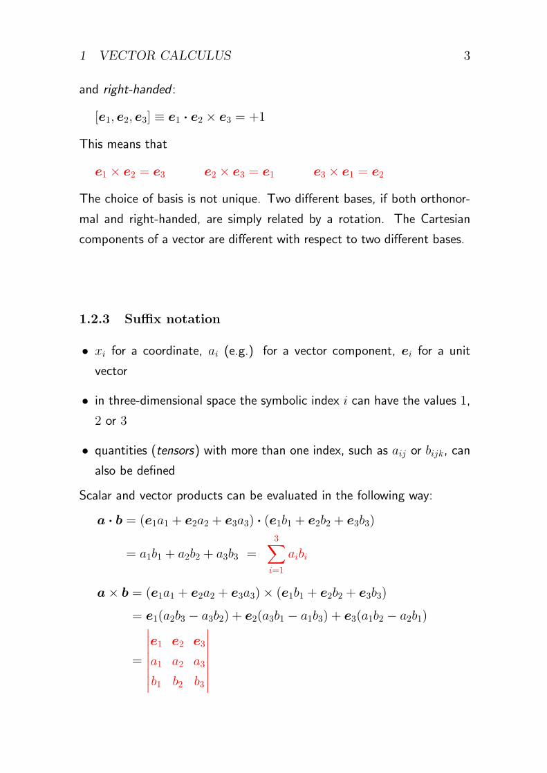
and right-handed :

[e1, e2, e3] ≡ e1 · e2 × e3 = +1

This means that

e1 × e2 = e3 e2 × e3 = e1 e3 × e1 = e2

The choice of basis is not unique. Two different bases, if both orthonor-

mal and right-handed, are simply related by a rotation. The Cartesian

components of a vector are different with respect to two different bases.

1.2.3 Suffix notation

• xi for a coordinate, ai (e.g.) for a vector component, ei for a unit

vector

• in three-dimensional space the symbolic index i can have the values 1,

2 or 3

• quantities (tensors) with more than one index, such as aij or bijk, can

also be defined

Scalar and vector products can be evaluated in the following way:

a · b = (e1a1 + e2a2 + e3a3) · (e1b1 + e2b2 + e3b3)

= a1b1 + a2b2 + a3b3 =3∑

i=1

aibi

a× b = (e1a1 + e2a2 + e3a3)× (e1b1 + e2b2 + e3b3)

= e1(a2b3 − a3b2) + e2(a3b1 − a1b3) + e3(a1b2 − a2b1)

=

∣∣∣∣∣∣∣∣e1 e2 e3

a1 a2 a3

b1 b2 b3

∣∣∣∣∣∣∣∣

1 VECTOR CALCULUS 4

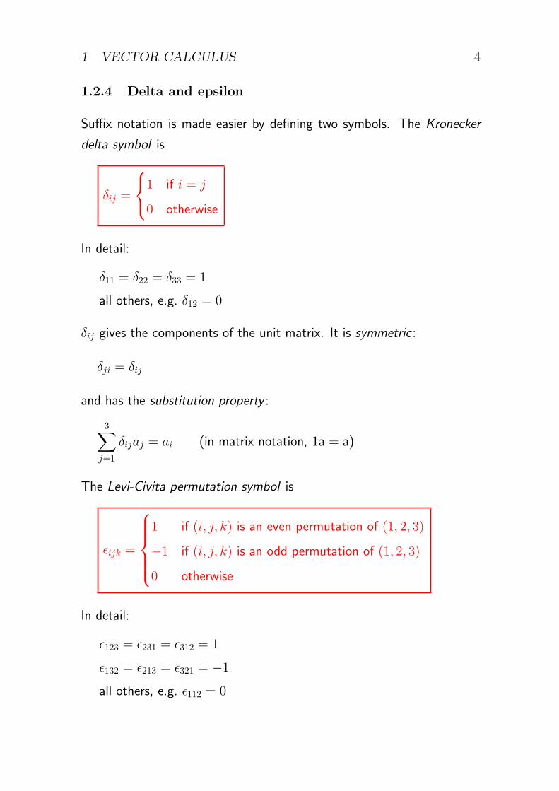
1.2.4 Delta and epsilon

Suffix notation is made easier by defining two symbols. The Kronecker

delta symbol is

δij =

1 if i = j

0 otherwise

In detail:

δ11 = δ22 = δ33 = 1

all others, e.g. δ12 = 0

δij gives the components of the unit matrix. It is symmetric :

δji = δij

and has the substitution property :

3∑j=1

δijaj = ai (in matrix notation, 1a = a)

The Levi-Civita permutation symbol is

ϵijk =

1 if (i, j, k) is an even permutation of (1, 2, 3)

−1 if (i, j, k) is an odd permutation of (1, 2, 3)

0 otherwise

In detail:

ϵ123 = ϵ231 = ϵ312 = 1

ϵ132 = ϵ213 = ϵ321 = −1

all others, e.g. ϵ112 = 0

1 VECTOR CALCULUS 5

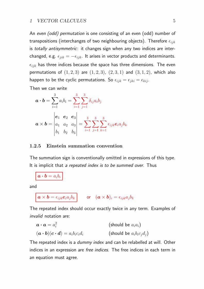
An even (odd) permutation is one consisting of an even (odd) number of

transpositions (interchanges of two neighbouring objects). Therefore ϵijk

is totally antisymmetric : it changes sign when any two indices are inter-

changed, e.g. ϵjik = −ϵijk. It arises in vector products and determinants.

ϵijk has three indices because the space has three dimensions. The even

permutations of (1, 2, 3) are (1, 2, 3), (2, 3, 1) and (3, 1, 2), which also

happen to be the cyclic permutations. So ϵijk = ϵjki = ϵkij.

Then we can write

a · b =3∑

i=1

aibi =3∑

i=1

3∑j=1

δijaibj

a× b =

∣∣∣∣∣∣∣∣e1 e2 e3

a1 a2 a3

b1 b2 b3

∣∣∣∣∣∣∣∣ =3∑

i=1

3∑j=1

3∑k=1

ϵijkeiajbk

1.2.5 Einstein summation convention

The summation sign is conventionally omitted in expressions of this type.

It is implicit that a repeated index is to be summed over. Thus

a · b = aibi

and

a× b = ϵijkeiajbk or (a× b)i = ϵijkajbk

The repeated index should occur exactly twice in any term. Examples of

invalid notation are:

a · a = a2i (should be aiai)

(a · b)(c · d) = aibicidi (should be aibicjdj)

The repeated index is a dummy index and can be relabelled at will. Other

indices in an expression are free indices. The free indices in each term in

an equation must agree.

1 VECTOR CALCULUS 6

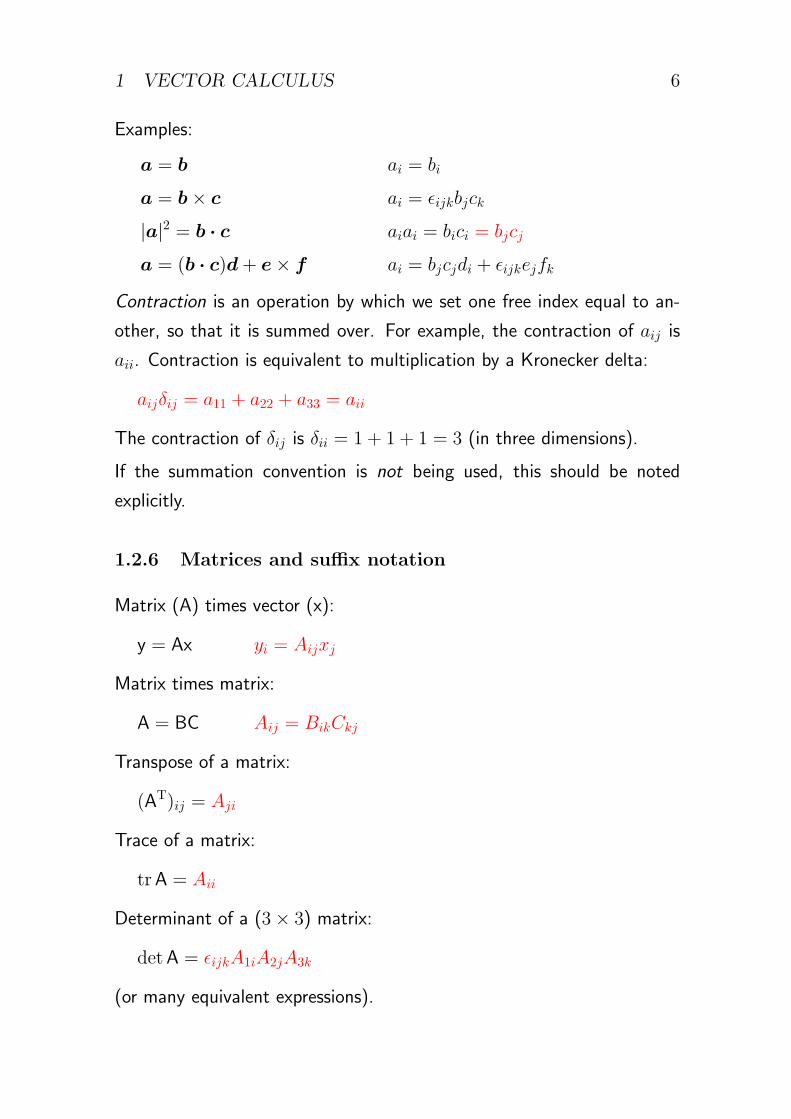
Examples:

a = b ai = bi

a = b× c ai = ϵijkbjck

|a|2 = b · c aiai = bici = bjcj

a = (b · c)d+ e× f ai = bjcjdi + ϵijkejfk

Contraction is an operation by which we set one free index equal to an-

other, so that it is summed over. For example, the contraction of aij is

aii. Contraction is equivalent to multiplication by a Kronecker delta:

aijδij = a11 + a22 + a33 = aii

The contraction of δij is δii = 1 + 1 + 1 = 3 (in three dimensions).

If the summation convention is not being used, this should be noted

explicitly.

1.2.6 Matrices and suffix notation

Matrix (A) times vector (x):

y = Ax yi = Aijxj

Matrix times matrix:

A = BC Aij = BikCkj

Transpose of a matrix:

(AT)ij = Aji

Trace of a matrix:

trA = Aii

Determinant of a (3× 3) matrix:

detA = ϵijkA1iA2jA3k

(or many equivalent expressions).

1 VECTOR CALCULUS 7

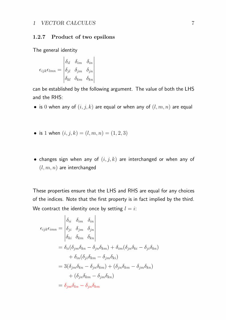
1.2.7 Product of two epsilons

The general identity

ϵijkϵlmn =

∣∣∣∣∣∣∣∣δil δim δin

δjl δjm δjn

δkl δkm δkn

∣∣∣∣∣∣∣∣can be established by the following argument. The value of both the LHS

and the RHS:

• is 0 when any of (i, j, k) are equal or when any of (l,m, n) are equal

• is 1 when (i, j, k) = (l,m, n) = (1, 2, 3)

• changes sign when any of (i, j, k) are interchanged or when any of

(l,m, n) are interchanged

These properties ensure that the LHS and RHS are equal for any choices

of the indices. Note that the first property is in fact implied by the third.

We contract the identity once by setting l = i:

ϵijkϵimn =

∣∣∣∣∣∣∣∣δii δim δin

δji δjm δjn

δki δkm δkn

∣∣∣∣∣∣∣∣= δii(δjmδkn − δjnδkm) + δim(δjnδki − δjiδkn)

+ δin(δjiδkm − δjmδki)

= 3(δjmδkn − δjnδkm) + (δjnδkm − δjmδkn)

+ (δjnδkm − δjmδkn)

= δjmδkn − δjnδkm

1 VECTOR CALCULUS 8

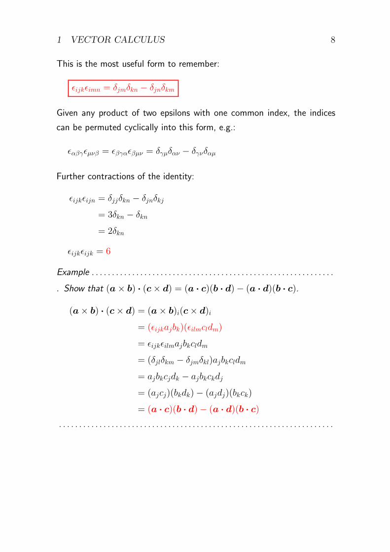
This is the most useful form to remember:

ϵijkϵimn = δjmδkn − δjnδkm

Given any product of two epsilons with one common index, the indices

can be permuted cyclically into this form, e.g.:

ϵαβγϵµνβ = ϵβγαϵβµν = δγµδαν − δγνδαµ

Further contractions of the identity:

ϵijkϵijn = δjjδkn − δjnδkj

= 3δkn − δkn

= 2δkn

ϵijkϵijk = 6

Example . . . . . . . . . . . . . . . . . . . . . . . . . . . . . . . . . . . . . . . . . . . . . . . . . . . . . . . . . . . .

▷ Show that (a× b) · (c× d) = (a · c)(b · d)− (a · d)(b · c).

(a× b) · (c× d) = (a× b)i(c× d)i

= (ϵijkajbk)(ϵilmcldm)

= ϵijkϵilmajbkcldm

= (δjlδkm − δjmδkl)ajbkcldm

= ajbkcjdk − ajbkckdj

= (ajcj)(bkdk)− (ajdj)(bkck)

= (a · c)(b · d)− (a · d)(b · c). . . . . . . . . . . . . . . . . . . . . . . . . . . . . . . . . . . . . . . . . . . . . . . . . . . . . . . . . . . . . . . . . . . .

1 VECTOR CALCULUS 9

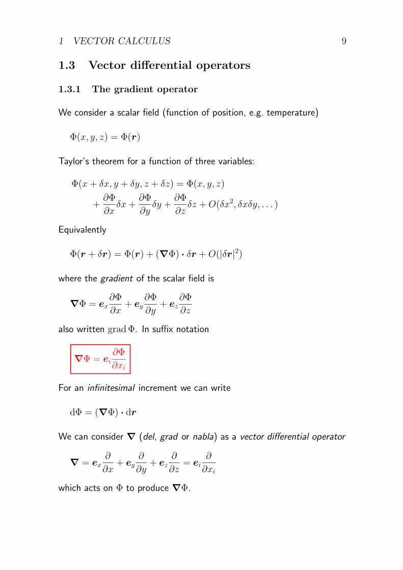
1.3 Vector differential operators

1.3.1 The gradient operator

We consider a scalar field (function of position, e.g. temperature)

Φ(x, y, z) = Φ(r)

Taylor’s theorem for a function of three variables:

Φ(x+ δx, y + δy, z + δz) = Φ(x, y, z)

+∂Φ

∂xδx+

∂Φ

∂yδy +

∂Φ

∂zδz +O(δx2, δxδy, . . . )

Equivalently

Φ(r + δr) = Φ(r) + (∇Φ) · δr +O(|δr|2)

where the gradient of the scalar field is

∇Φ = ex∂Φ

∂x+ ey

∂Φ

∂y+ ez

∂Φ

∂z

also written gradΦ. In suffix notation

∇Φ = ei∂Φ

∂xi

For an infinitesimal increment we can write

dΦ = (∇Φ) · dr

We can consider ∇ (del, grad or nabla) as a vector differential operator

∇ = ex∂

∂x+ ey

∂

∂y+ ez

∂

∂z= ei

∂

∂xi

which acts on Φ to produce ∇Φ.

1 VECTOR CALCULUS 10

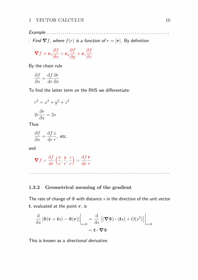
Example . . . . . . . . . . . . . . . . . . . . . . . . . . . . . . . . . . . . . . . . . . . . . . . . . . . . . . . . . . . .

▷ Find ∇f , where f(r) is a function of r = |r|. By definition

∇f = ex∂f

∂x+ ey

∂f

∂y+ ez

∂f

∂z

By the chain rule

∂f

∂x=

df

dr

∂r

∂x

To find the latter term on the RHS we differentiate:

r2 = x2 + y2 + z2

2r∂r

∂x= 2x

Thus

∂f

∂x=

df

dr

x

r, etc.

and

∇f =df

dr

(xr,y

r,z

r

)=

df

dr

r

r

. . . . . . . . . . . . . . . . . . . . . . . . . . . . . . . . . . . . . . . . . . . . . . . . . . . . . . . . . . . . . . . . . . . .

1.3.2 Geometrical meaning of the gradient

The rate of change of Φ with distance s in the direction of the unit vector

t, evaluated at the point r, is

d

ds[Φ(r + ts)− Φ(r)]

∣∣∣∣s=0

=d

ds

[(∇Φ) · (ts) +O(s2)

]∣∣∣∣s=0

= t · ∇Φ

This is known as a directional derivative.

1 VECTOR CALCULUS 11

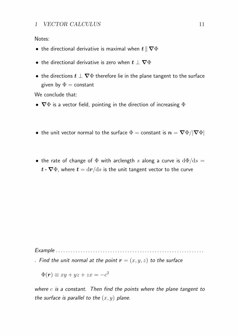
Notes:

• the directional derivative is maximal when t ∥∇Φ

• the directional derivative is zero when t ⊥ ∇Φ

• the directions t ⊥ ∇Φ therefore lie in the plane tangent to the surface

given by Φ = constant

We conclude that:

• ∇Φ is a vector field, pointing in the direction of increasing Φ

• the unit vector normal to the surface Φ = constant is n = ∇Φ/|∇Φ|

• the rate of change of Φ with arclength s along a curve is dΦ/ds =

t · ∇Φ, where t = dr/ds is the unit tangent vector to the curve

Example . . . . . . . . . . . . . . . . . . . . . . . . . . . . . . . . . . . . . . . . . . . . . . . . . . . . . . . . . . . .

▷ Find the unit normal at the point r = (x, y, z) to the surface

Φ(r) ≡ xy + yz + zx = −c2

where c is a constant. Then find the points where the plane tangent to

the surface is parallel to the (x, y) plane.

1 VECTOR CALCULUS 12

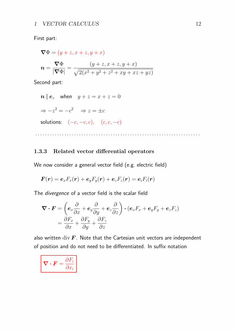
First part:

∇Φ = (y + z, x+ z, y + x)

n =∇Φ

|∇Φ|=

(y + z, x+ z, y + x)√2(x2 + y2 + z2 + xy + xz + yz)

Second part:

n ∥ ez when y + z = x+ z = 0

⇒ −z2 = −c2 ⇒ z = ±c

solutions: (−c,−c, c), (c, c,−c)

. . . . . . . . . . . . . . . . . . . . . . . . . . . . . . . . . . . . . . . . . . . . . . . . . . . . . . . . . . . . . . . . . . . .

1.3.3 Related vector differential operators

We now consider a general vector field (e.g. electric field)

F (r) = exFx(r) + eyFy(r) + ezFz(r) = eiFi(r)

The divergence of a vector field is the scalar field

∇ · F =

(ex

∂

∂x+ ey

∂

∂y+ ez

∂

∂z

)· (exFx + eyFy + ezFz)

=∂Fx

∂x+∂Fy

∂y+∂Fz

∂z

also written divF . Note that the Cartesian unit vectors are independent

of position and do not need to be differentiated. In suffix notation

∇ · F =∂Fi

∂xi

1 VECTOR CALCULUS 13

The curl of a vector field is the vector field

∇× F =

(ex

∂

∂x+ ey

∂

∂y+ ez

∂

∂z

)× (exFx + eyFy + ezFz)

= ex

(∂Fz

∂y− ∂Fy

∂z

)+ ey

(∂Fx

∂z− ∂Fz

∂x

)+ ez

(∂Fy

∂x− ∂Fx

∂y

)

=

∣∣∣∣∣∣∣∣ex ey ez

∂/∂x ∂/∂y ∂/∂z

Fx Fy Fz

∣∣∣∣∣∣∣∣also written curlF . In suffix notation

∇× F = eiϵijk∂Fk

∂xjor (∇× F )i = ϵijk

∂Fk

∂xj

The Laplacian of a scalar field is the scalar field

∇2Φ = ∇ · (∇Φ) =∂2Φ

∂x2+∂2Φ

∂y2+∂2Φ

∂z2=

∂2Φ

∂xi∂xi

The Laplacian differential operator (del squared) is

∇2 =∂2

∂x2+

∂2

∂y2+

∂2

∂z2=

∂2

∂xi∂xi

It appears very commonly in partial differential equations. The Laplacian

of a vector field can also be defined. In suffix notation

∇2F = ei∂2Fi

∂xj∂xj

because the Cartesian unit vectors are independent of position.

The directional derivative operator is

t · ∇ = tx∂

∂x+ ty

∂

∂y+ tz

∂

∂z= ti

∂

∂xi

t · ∇Φ is the rate of change of Φ with distance in the direction of the

unit vector t. This can be thought of either as t · (∇Φ) or as (t · ∇)Φ.

1 VECTOR CALCULUS 14

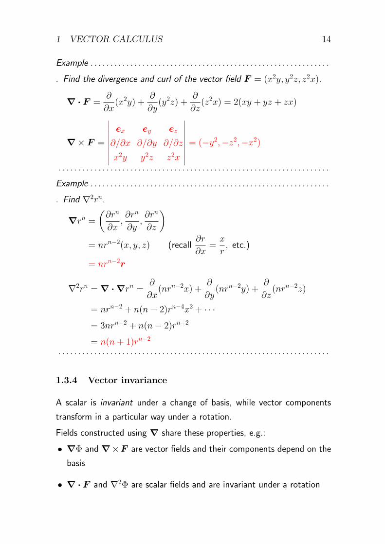
Example . . . . . . . . . . . . . . . . . . . . . . . . . . . . . . . . . . . . . . . . . . . . . . . . . . . . . . . . . . . .

▷ Find the divergence and curl of the vector field F = (x2y, y2z, z2x).

∇ · F =∂

∂x(x2y) +

∂

∂y(y2z) +

∂

∂z(z2x) = 2(xy + yz + zx)

∇× F =

∣∣∣∣∣∣∣∣ex ey ez

∂/∂x ∂/∂y ∂/∂z

x2y y2z z2x

∣∣∣∣∣∣∣∣ = (−y2,−z2,−x2)

. . . . . . . . . . . . . . . . . . . . . . . . . . . . . . . . . . . . . . . . . . . . . . . . . . . . . . . . . . . . . . . . . . . .

Example . . . . . . . . . . . . . . . . . . . . . . . . . . . . . . . . . . . . . . . . . . . . . . . . . . . . . . . . . . . .

▷ Find ∇2rn.

∇rn =

(∂rn

∂x,∂rn

∂y,∂rn

∂z

)= nrn−2(x, y, z) (recall

∂r

∂x=x

r, etc.)

= nrn−2r

∇2rn = ∇ ·∇rn =∂

∂x(nrn−2x) +

∂

∂y(nrn−2y) +

∂

∂z(nrn−2z)

= nrn−2 + n(n− 2)rn−4x2 + · · ·

= 3nrn−2 + n(n− 2)rn−2

= n(n+ 1)rn−2

. . . . . . . . . . . . . . . . . . . . . . . . . . . . . . . . . . . . . . . . . . . . . . . . . . . . . . . . . . . . . . . . . . . .

1.3.4 Vector invariance

A scalar is invariant under a change of basis, while vector components

transform in a particular way under a rotation.

Fields constructed using ∇ share these properties, e.g.:

• ∇Φ and ∇×F are vector fields and their components depend on the

basis

• ∇ · F and ∇2Φ are scalar fields and are invariant under a rotation

1 VECTOR CALCULUS 15

grad, div and ∇2 can be defined in spaces of any dimension, but curl

(like the vector product) is a three-dimensional concept.

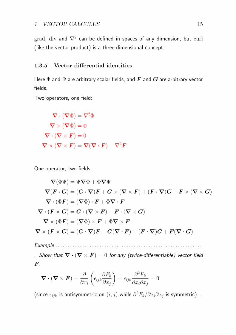
1.3.5 Vector differential identities

Here Φ and Ψ are arbitrary scalar fields, and F and G are arbitrary vector

fields.

Two operators, one field:

∇ · (∇Φ) = ∇2Φ

∇× (∇Φ) = 0

∇ · (∇× F ) = 0

∇× (∇× F ) = ∇(∇ · F )−∇2F

One operator, two fields:

∇(ΦΨ) = Ψ∇Φ + Φ∇Ψ

∇(F ·G) = (G · ∇)F +G× (∇× F ) + (F · ∇)G+ F × (∇×G)

∇ · (ΦF ) = (∇Φ) · F + Φ∇ · F

∇ · (F ×G) = G · (∇× F )− F · (∇×G)

∇× (ΦF ) = (∇Φ)× F + Φ∇× F

∇× (F ×G) = (G · ∇)F −G(∇ · F )− (F · ∇)G+ F (∇ ·G)

Example . . . . . . . . . . . . . . . . . . . . . . . . . . . . . . . . . . . . . . . . . . . . . . . . . . . . . . . . . . . .

▷ Show that ∇ · (∇ × F ) = 0 for any (twice-differentiable) vector field

F .

∇ · (∇× F ) =∂

∂xi

(ϵijk

∂Fk

∂xj

)= ϵijk

∂2Fk

∂xi∂xj= 0

(since ϵijk is antisymmetric on (i, j) while ∂2Fk/∂xi∂xj is symmetric) .

1 VECTOR CALCULUS 16

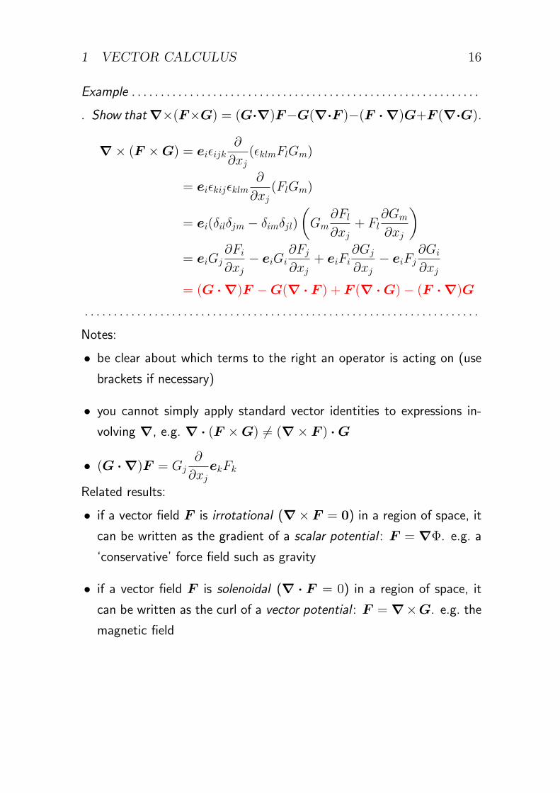
Example . . . . . . . . . . . . . . . . . . . . . . . . . . . . . . . . . . . . . . . . . . . . . . . . . . . . . . . . . . . .

▷ Show that∇×(F×G) = (G·∇)F−G(∇·F )−(F · ∇)G+F (∇·G).

∇× (F ×G) = eiϵijk∂

∂xj(ϵklmFlGm)

= eiϵkijϵklm∂

∂xj(FlGm)

= ei(δilδjm − δimδjl)

(Gm

∂Fl

∂xj+ Fl

∂Gm

∂xj

)= eiGj

∂Fi

∂xj− eiGi

∂Fj

∂xj+ eiFi

∂Gj

∂xj− eiFj

∂Gi

∂xj

= (G · ∇)F −G(∇ · F ) + F (∇ ·G)− (F · ∇)G

. . . . . . . . . . . . . . . . . . . . . . . . . . . . . . . . . . . . . . . . . . . . . . . . . . . . . . . . . . . . . . . . . . . .

Notes:

• be clear about which terms to the right an operator is acting on (use

brackets if necessary)

• you cannot simply apply standard vector identities to expressions in-

volving ∇, e.g. ∇ · (F ×G) = (∇× F ) ·G

• (G · ∇)F = Gj∂

∂xjekFk

Related results:

• if a vector field F is irrotational (∇×F = 0) in a region of space, it

can be written as the gradient of a scalar potential : F = ∇Φ. e.g. a

‘conservative’ force field such as gravity

• if a vector field F is solenoidal (∇ · F = 0) in a region of space, it

can be written as the curl of a vector potential : F = ∇×G. e.g. the

magnetic field

1 VECTOR CALCULUS 17

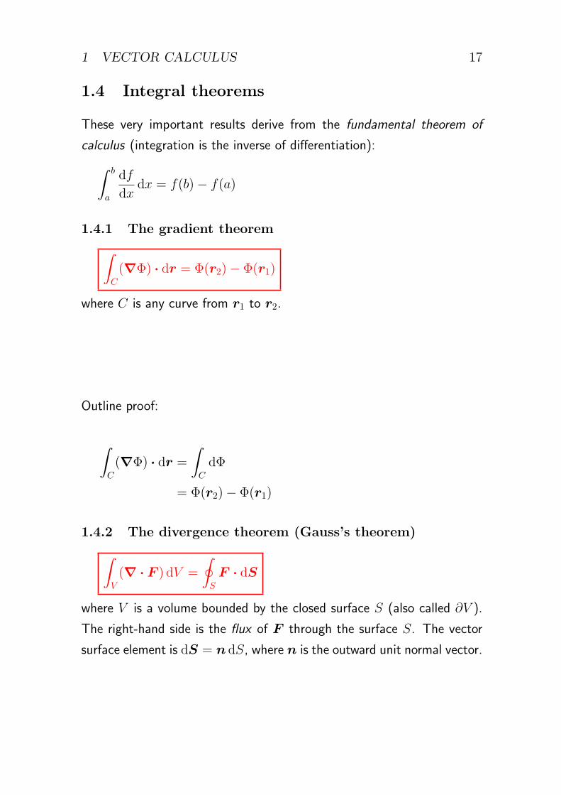
1.4 Integral theorems

These very important results derive from the fundamental theorem of

calculus (integration is the inverse of differentiation):∫ b

a

df

dxdx = f(b)− f(a)

1.4.1 The gradient theorem∫C

(∇Φ) · dr = Φ(r2)− Φ(r1)

where C is any curve from r1 to r2.

Outline proof:

∫C

(∇Φ) · dr =

∫C

dΦ

= Φ(r2)− Φ(r1)

1.4.2 The divergence theorem (Gauss’s theorem)∫V

(∇ · F ) dV =

∮S

F · dS

where V is a volume bounded by the closed surface S (also called ∂V ).

The right-hand side is the flux of F through the surface S. The vector

surface element is dS = n dS, where n is the outward unit normal vector.

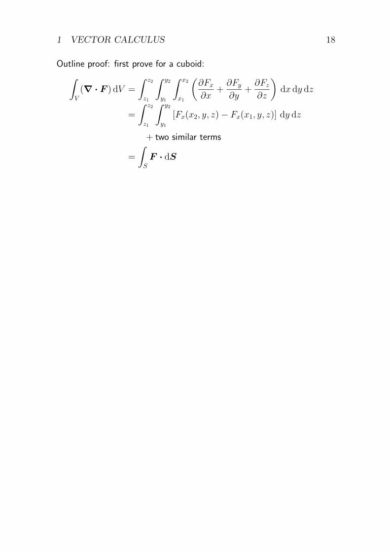
1 VECTOR CALCULUS 18

Outline proof: first prove for a cuboid:∫V

(∇ · F ) dV =

∫ z2

z1

∫ y2

y1

∫ x2

x1

(∂Fx

∂x+∂Fy

∂y+∂Fz

∂z

)dx dy dz

=

∫ z2

z1

∫ y2

y1

[Fx(x2, y, z)− Fx(x1, y, z)] dy dz

+ two similar terms

=

∫S

F · dS

1 VECTOR CALCULUS 19

An arbitrary volume V can be subdivided into small cuboids to any desired

accuracy. When the integrals are added together, the fluxes through

internal surfaces cancel out, leaving only the flux through S.

A simply connected volume (e.g. a ball) is one with no holes. It has only

an outer surface. A multiply connected volume (e.g. a spherical shell)

may have more than one surface; all the surfaces must be considered.

1 VECTOR CALCULUS 20

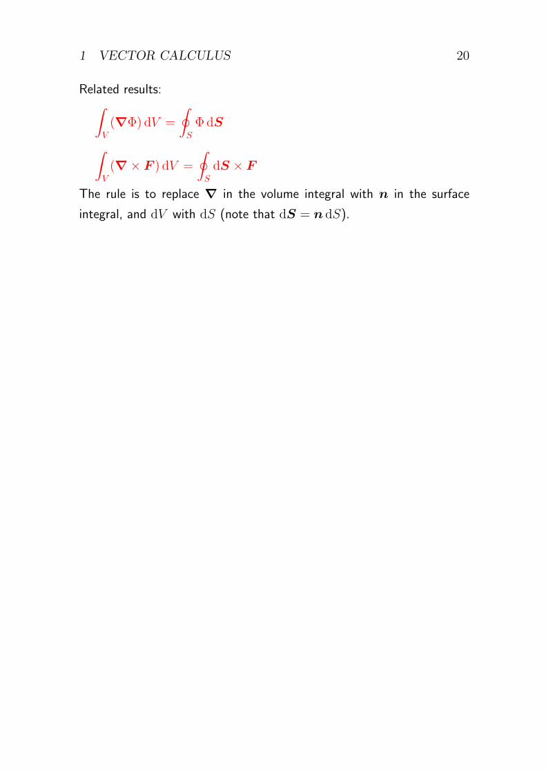
Related results:∫V

(∇Φ) dV =

∮S

ΦdS

∫V

(∇× F ) dV =

∮S

dS × F

The rule is to replace ∇ in the volume integral with n in the surface

integral, and dV with dS (note that dS = n dS).

1 VECTOR CALCULUS 21

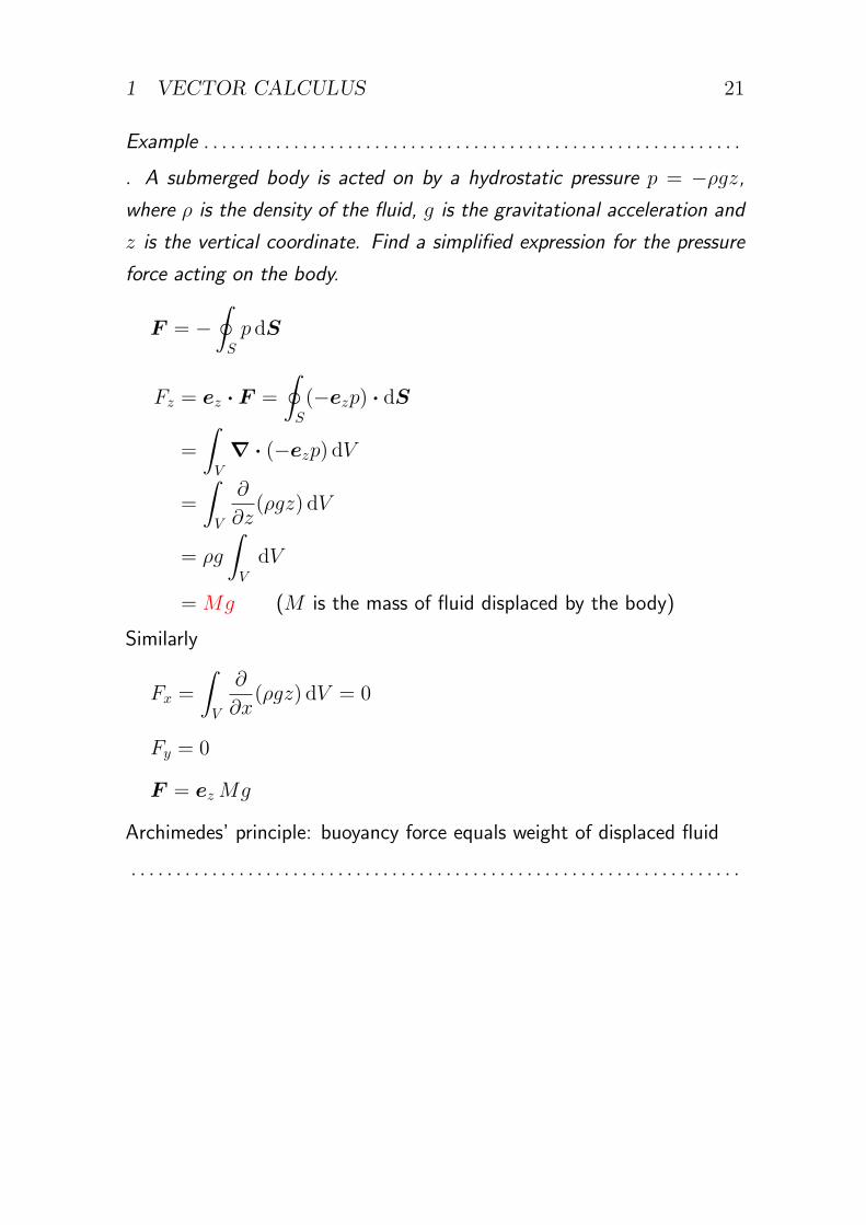
Example . . . . . . . . . . . . . . . . . . . . . . . . . . . . . . . . . . . . . . . . . . . . . . . . . . . . . . . . . . . .

▷ A submerged body is acted on by a hydrostatic pressure p = −ρgz,where ρ is the density of the fluid, g is the gravitational acceleration and

z is the vertical coordinate. Find a simplified expression for the pressure

force acting on the body.

F = −∮S

p dS

Fz = ez · F =

∮S

(−ezp) · dS

=

∫V

∇ · (−ezp) dV

=

∫V

∂

∂z(ρgz) dV

= ρg

∫V

dV

=Mg (M is the mass of fluid displaced by the body)

Similarly

Fx =

∫V

∂

∂x(ρgz) dV = 0

Fy = 0

F = ezMg

Archimedes’ principle: buoyancy force equals weight of displaced fluid

. . . . . . . . . . . . . . . . . . . . . . . . . . . . . . . . . . . . . . . . . . . . . . . . . . . . . . . . . . . . . . . . . . . .

1 VECTOR CALCULUS 22

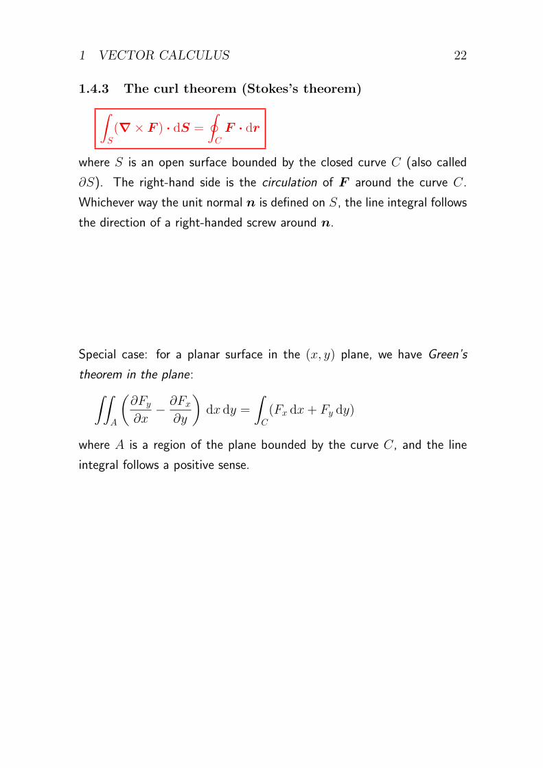
1.4.3 The curl theorem (Stokes’s theorem)∫S

(∇× F ) · dS =

∮C

F · dr

where S is an open surface bounded by the closed curve C (also called

∂S). The right-hand side is the circulation of F around the curve C.

Whichever way the unit normal n is defined on S, the line integral follows

the direction of a right-handed screw around n.

Special case: for a planar surface in the (x, y) plane, we have Green’s

theorem in the plane:∫∫A

(∂Fy

∂x− ∂Fx

∂y

)dx dy =

∫C

(Fx dx+ Fy dy)

where A is a region of the plane bounded by the curve C, and the line

integral follows a positive sense.

1 VECTOR CALCULUS 23

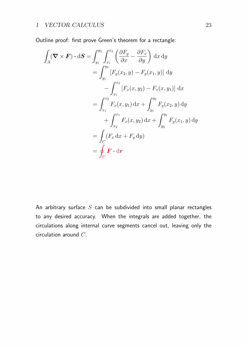
Outline proof: first prove Green’s theorem for a rectangle:∫A

(∇× F ) · dS =

∫ y2

y1

∫ x2

x1

(∂Fy

∂x− ∂Fx

∂y

)dx dy

=

∫ y2

y1

[Fy(x2, y)− Fy(x1, y)] dy

−∫ x2

x1

[Fx(x, y2)− Fx(x, y1)] dx

=

∫ x2

x1

Fx(x, y1) dx+

∫ y2

y1

Fy(x2, y) dy

+

∫ x1

x2

Fx(x, y2) dx+

∫ y1

y2

Fy(x1, y) dy

=

∫C

(Fx dx+ Fy dy)

=

∮C

F · dr

An arbitrary surface S can be subdivided into small planar rectangles

to any desired accuracy. When the integrals are added together, the

circulations along internal curve segments cancel out, leaving only the

circulation around C.

1 VECTOR CALCULUS 24

Notes:

• in Stokes’s theorem S is an open surface, while in Gauss’s theorem it

is closed

• many different surfaces are bounded by the same closed curve, while

only one volume is bounded by a closed surface

• a multiply connected surface (e.g. an annulus) may have more than

one bounding curve

1.4.4 Geometrical definitions of grad, div and curl

The integral theorems can be used to assign coordinate-independent mean-

ings to grad, div and curl.

Apply the gradient theorem to an arbitrarily small line segment δr = t δs

in the direction of any unit vector t. Since the variation of ∇Φ and t

along the line segment is negligible,

(∇Φ) · t δs ≈ δΦ

and so

t · (∇Φ) = limδs→0

δΦ

δs

This definition can be used to determine the component of ∇Φ in any

desired direction.

1 VECTOR CALCULUS 25

Similarly, by applying the divergence theorem to an arbitrarily small volume

δV bounded by a surface δS, we find that

∇ · F = limδV→0

1

δV

∫δS

F · dS

Finally, by applying the curl theorem to an arbitrarily small open surface

δS with unit normal vector n and bounded by a curve δC, we find that

n · (∇× F ) = limδS→0

1

δS

∫δC

F · dr

The gradient therefore describes the rate of change of a scalar field with

distance. The divergence describes the net source or efflux of a vector

field per unit volume. The curl describes the circulation or rotation of a

vector field per unit area.

1.5 Orthogonal curvilinear coordinates

Cartesian coordinates can be replaced with any independent set of co-

ordinates q1(x1, x2, x3), q2(x1, x2, x3), q3(x1, x2, x3), e.g. cylindrical or

spherical polar coordinates.

Curvilinear (as opposed to rectilinear) means that the coordinate ‘axes’ are

curves. Curvilinear coordinates are useful for solving problems in curved

geometry (e.g. geophysics).

1.5.1 Line element

The infinitesimal line element in Cartesian coordinates is

dr = ex dx+ ey dy + ez dz

In general curvilinear coordinates we have

dr = h1 dq1 + h2 dq2 + h3 dq3

1 VECTOR CALCULUS 26

where

hi = eihi =∂r

∂qi(no sum)

determines the displacement associated with an increment of the coordi-

nate qi.

hi = |hi| is the scale factor (or metric coefficient) associated with the

coordinate qi. It converts a coordinate increment into a length. Any point

at which hi = 0 is a coordinate singularity at which the coordinate system

breaks down.

ei is the corresponding unit vector. This notation generalizes the use of

ei for a Cartesian unit vector. For Cartesian coordinates, hi = 1 and ei

are constant, but in general both hi and ei depend on position.

The Einstein summation convention does not work well with orthogonal

curvilinear coordinates.

1.5.2 The Jacobian

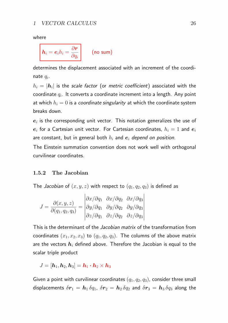
The Jacobian of (x, y, z) with respect to (q1, q2, q3) is defined as

J =∂(x, y, z)

∂(q1, q2, q3)=

∣∣∣∣∣∣∣∣∂x/∂q1 ∂x/∂q2 ∂x/∂q3

∂y/∂q1 ∂y/∂q2 ∂y/∂q3

∂z/∂q1 ∂z/∂q2 ∂z/∂q3

∣∣∣∣∣∣∣∣This is the determinant of the Jacobian matrix of the transformation from

coordinates (x1, x2, x3) to (q1, q2, q3). The columns of the above matrix

are the vectors hi defined above. Therefore the Jacobian is equal to the

scalar triple product

J = [h1,h2,h3] = h1 · h2 × h3

Given a point with curvilinear coordinates (q1, q2, q3), consider three small

displacements δr1 = h1 δq1, δr2 = h2 δq2 and δr3 = h3 δq3 along the

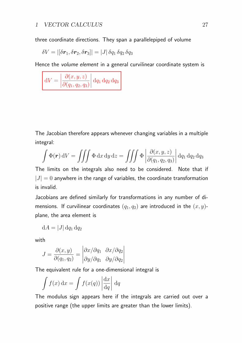
1 VECTOR CALCULUS 27

three coordinate directions. They span a parallelepiped of volume

δV = |[δr1, δr2, δr3]| = |J | δq1 δq2 δq3

Hence the volume element in a general curvilinear coordinate system is

dV =

∣∣∣∣ ∂(x, y, z)∂(q1, q2, q3)

∣∣∣∣ dq1 dq2 dq3

The Jacobian therefore appears whenever changing variables in a multiple

integral:∫Φ(r) dV =

∫∫∫Φdx dy dz =

∫∫∫Φ

∣∣∣∣ ∂(x, y, z)∂(q1, q2, q3)

∣∣∣∣ dq1 dq2 dq3The limits on the integrals also need to be considered. Note that if

|J | = 0 anywhere in the range of variables, the coordinate transformation

is invalid.

Jacobians are defined similarly for transformations in any number of di-

mensions. If curvilinear coordinates (q1, q2) are introduced in the (x, y)-

plane, the area element is

dA = |J | dq1 dq2

with

J =∂(x, y)

∂(q1, q2)=

∣∣∣∣∣∂x/∂q1 ∂x/∂q2

∂y/∂q1 ∂y/∂q2

∣∣∣∣∣The equivalent rule for a one-dimensional integral is∫

f(x) dx =

∫f(x(q))

∣∣∣∣dxdq∣∣∣∣ dq

The modulus sign appears here if the integrals are carried out over a

positive range (the upper limits are greater than the lower limits).

1 VECTOR CALCULUS 28

1.5.3 Properties of Jacobians

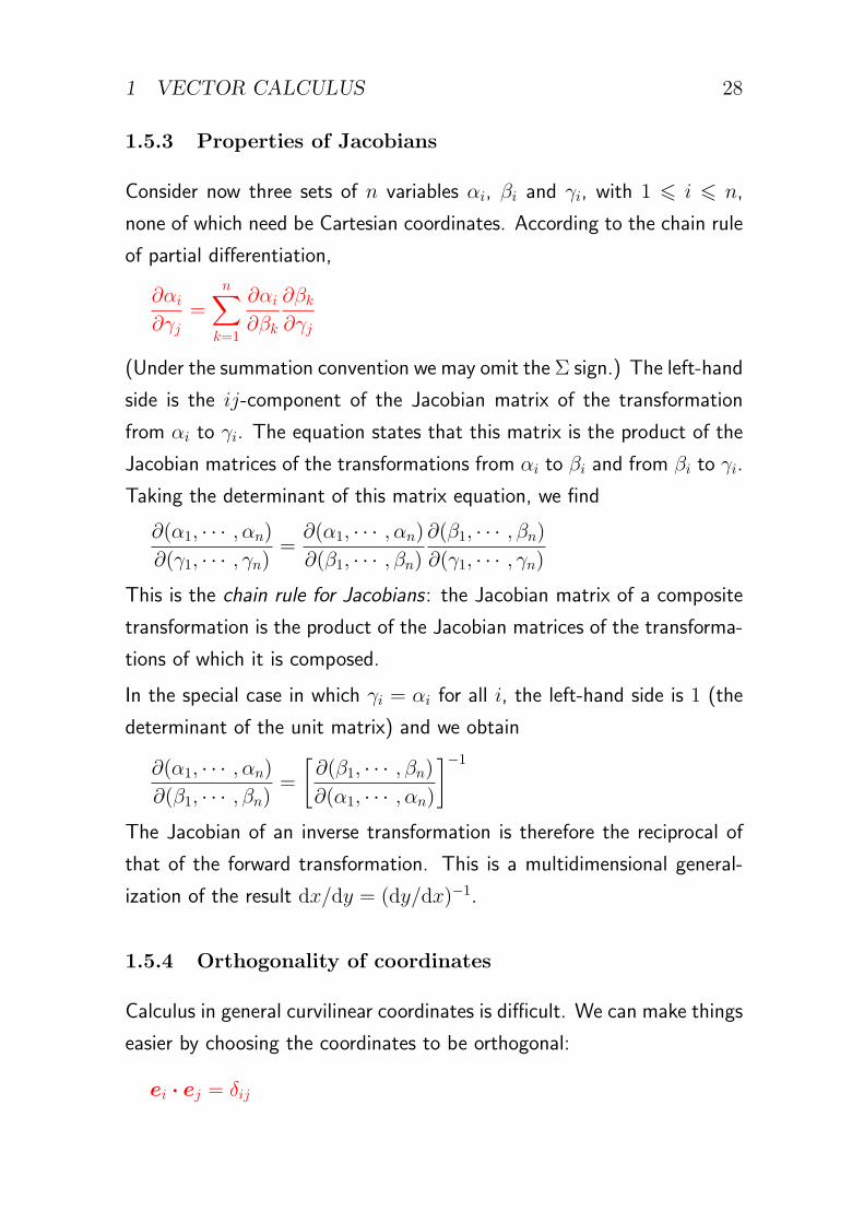
Consider now three sets of n variables αi, βi and γi, with 1 ⩽ i ⩽ n,

none of which need be Cartesian coordinates. According to the chain rule

of partial differentiation,

∂αi

∂γj=

n∑k=1

∂αi

∂βk

∂βk∂γj

(Under the summation convention we may omit the Σ sign.) The left-hand

side is the ij-component of the Jacobian matrix of the transformation

from αi to γi. The equation states that this matrix is the product of the

Jacobian matrices of the transformations from αi to βi and from βi to γi.

Taking the determinant of this matrix equation, we find

∂(α1, · · · , αn)

∂(γ1, · · · , γn)=∂(α1, · · · , αn)

∂(β1, · · · , βn)∂(β1, · · · , βn)∂(γ1, · · · , γn)

This is the chain rule for Jacobians: the Jacobian matrix of a composite

transformation is the product of the Jacobian matrices of the transforma-

tions of which it is composed.

In the special case in which γi = αi for all i, the left-hand side is 1 (the

determinant of the unit matrix) and we obtain

∂(α1, · · · , αn)

∂(β1, · · · , βn)=

[∂(β1, · · · , βn)∂(α1, · · · , αn)

]−1

The Jacobian of an inverse transformation is therefore the reciprocal of

that of the forward transformation. This is a multidimensional general-

ization of the result dx/dy = (dy/dx)−1.

1.5.4 Orthogonality of coordinates

Calculus in general curvilinear coordinates is difficult. We can make things

easier by choosing the coordinates to be orthogonal:

ei · ej = δij

1 VECTOR CALCULUS 29

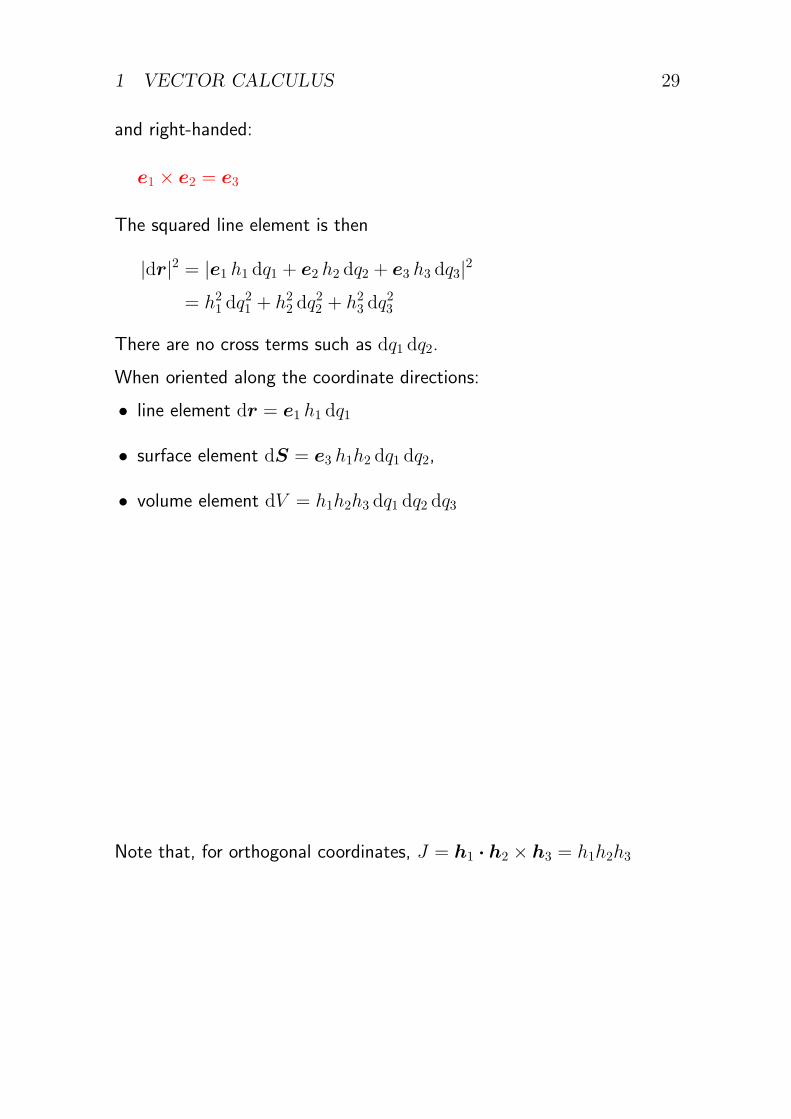
and right-handed:

e1 × e2 = e3

The squared line element is then

|dr|2 = |e1 h1 dq1 + e2 h2 dq2 + e3 h3 dq3|2

= h21 dq21 + h22 dq

22 + h23 dq

23

There are no cross terms such as dq1 dq2.

When oriented along the coordinate directions:

• line element dr = e1 h1 dq1

• surface element dS = e3 h1h2 dq1 dq2,

• volume element dV = h1h2h3 dq1 dq2 dq3

Note that, for orthogonal coordinates, J = h1 · h2 × h3 = h1h2h3

1 VECTOR CALCULUS 30

1.5.5 Commonly used orthogonal coordinate systems

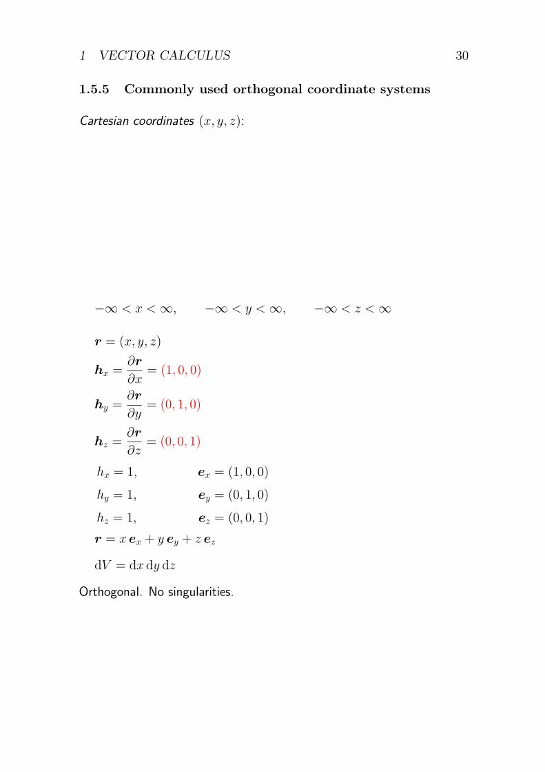
Cartesian coordinates (x, y, z):

−∞ < x <∞, −∞ < y <∞, −∞ < z <∞

r = (x, y, z)

hx =∂r

∂x= (1, 0, 0)

hy =∂r

∂y= (0, 1, 0)

hz =∂r

∂z= (0, 0, 1)

hx = 1, ex = (1, 0, 0)

hy = 1, ey = (0, 1, 0)

hz = 1, ez = (0, 0, 1)

r = x ex + y ey + z ez

dV = dx dy dz

Orthogonal. No singularities.

1 VECTOR CALCULUS 31

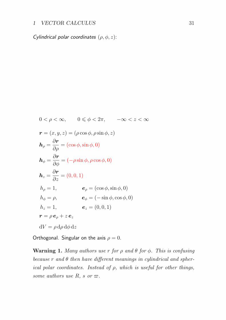
Cylindrical polar coordinates (ρ, ϕ, z):

0 < ρ <∞, 0 ⩽ ϕ < 2π, −∞ < z <∞

r = (x, y, z) = (ρ cosϕ, ρ sinϕ, z)

hρ =∂r

∂ρ= (cosϕ, sinϕ, 0)

hϕ =∂r

∂ϕ= (−ρ sinϕ, ρ cosϕ, 0)

hz =∂r

∂z= (0, 0, 1)

hρ = 1, eρ = (cosϕ, sinϕ, 0)

hϕ = ρ, eϕ = (− sinϕ, cosϕ, 0)

hz = 1, ez = (0, 0, 1)

r = ρ eρ + z ez

dV = ρ dρ dϕ dz

Orthogonal. Singular on the axis ρ = 0.

Warning 1. Many authors use r for ρ and θ for ϕ. This is confusing

because r and θ then have different meanings in cylindrical and spher-

ical polar coordinates. Instead of ρ, which is useful for other things,

some authors use R, s or ϖ.

1 VECTOR CALCULUS 32

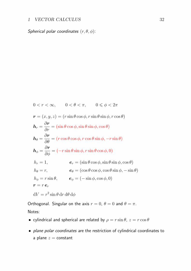
Spherical polar coordinates (r, θ, ϕ):

0 < r <∞, 0 < θ < π, 0 ⩽ ϕ < 2π

r = (x, y, z) = (r sin θ cosϕ, r sin θ sinϕ, r cos θ)

hr =∂r

∂r= (sin θ cosϕ, sin θ sinϕ, cos θ)

hθ =∂r

∂θ= (r cos θ cosϕ, r cos θ sinϕ,−r sin θ)

hϕ =∂r

∂ϕ= (−r sin θ sinϕ, r sin θ cosϕ, 0)

hr = 1, er = (sin θ cosϕ, sin θ sinϕ, cos θ)

hθ = r, eθ = (cos θ cosϕ, cos θ sinϕ,− sin θ)

hϕ = r sin θ, eϕ = (− sinϕ, cosϕ, 0)

r = r er

dV = r2 sin θ dr dθ dϕ

Orthogonal. Singular on the axis r = 0, θ = 0 and θ = π.

Notes:

• cylindrical and spherical are related by ρ = r sin θ, z = r cos θ

• plane polar coordinates are the restriction of cylindrical coordinates to

a plane z = constant

1 VECTOR CALCULUS 33

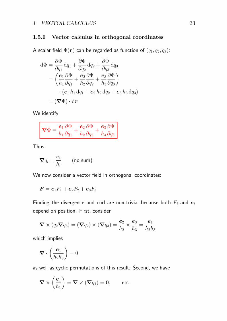
1.5.6 Vector calculus in orthogonal coordinates

A scalar field Φ(r) can be regarded as function of (q1, q2, q3):

dΦ =∂Φ

∂q1dq1 +

∂Φ

∂q2dq2 +

∂Φ

∂q3dq3

=

(e1h1

∂Φ

∂q1+

e2h2

∂Φ

∂q2+

e3h3

∂Φ

∂q3

)· (e1 h1 dq1 + e2 h2 dq2 + e3 h3 dq3)

= (∇Φ) · dr

We identify

∇Φ =e1h1

∂Φ

∂q1+

e2h2

∂Φ

∂q2+

e3h3

∂Φ

∂q3

Thus

∇qi =eihi

(no sum)

We now consider a vector field in orthogonal coordinates:

F = e1F1 + e2F2 + e3F3

Finding the divergence and curl are non-trivial because both Fi and ei

depend on position. First, consider

∇× (q2∇q3) = (∇q2)× (∇q3) =e2h2

× e3h3

=e1h2h3

which implies

∇ ·(

e1h2h3

)= 0

as well as cyclic permutations of this result. Second, we have

∇×(e1h1

)= ∇× (∇q1) = 0, etc.

1 VECTOR CALCULUS 34

Now, to work out ∇ · F , write

F =

(e1h2h3

)(h2h3F1) + · · · cyclic permutations

∇ · F =

(e1h2h3

)· ∇(h2h3F1) + · · ·

=

(e1h2h3

)·[e1h1

∂

∂q1(h2h3F1) +

e2h2

∂

∂q2(h2h3F1)

+e3h3

∂

∂q3(h2h3F1)

]+ · · ·

=1

h1h2h3

∂

∂q1(h2h3F1) + · · · cyclic permutations

Similarly, to work out ∇× F , write

F =

(e1h1

)(h1F1) + · · · cyclic permutations

∇× F = ∇(h1F1)×(e1h1

)+ · · ·

=

[e1h1

∂

∂q1(h1F1) +

e2h2

∂

∂q2(h1F1) +

e3h3

∂

∂q3(h1F1)

]×

(e1h1

)+ · · ·

=

[e2h1h3

∂

∂q3(h1F1)−

e3h1h2

∂

∂q2(h1F1)

]+ · · · cyclic permutations

The appearance of the scale factors inside the derivatives can be under-

stood with reference to the geometrical definitions of grad, div and curl:

t · (∇Φ) = limδs→0

δΦ

δs

∇ · F = limδV→0

1

δV

∫δS

F · dS

n · (∇× F ) = limδS→0

1

δS

∫δC

F · dr

1 VECTOR CALCULUS 35

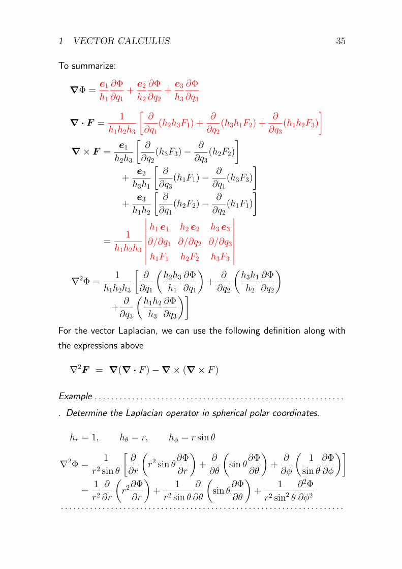
To summarize:

∇Φ =e1h1

∂Φ

∂q1+

e2h2

∂Φ

∂q2+

e3h3

∂Φ

∂q3

∇ · F =1

h1h2h3

[∂

∂q1(h2h3F1) +

∂

∂q2(h3h1F2) +

∂

∂q3(h1h2F3)

]∇× F =

e1h2h3

[∂

∂q2(h3F3)−

∂

∂q3(h2F2)

]+

e2h3h1

[∂

∂q3(h1F1)−

∂

∂q1(h3F3)

]+

e3h1h2

[∂

∂q1(h2F2)−

∂

∂q2(h1F1)

]

=1

h1h2h3

∣∣∣∣∣∣∣∣h1 e1 h2 e2 h3 e3

∂/∂q1 ∂/∂q2 ∂/∂q3

h1F1 h2F2 h3F3

∣∣∣∣∣∣∣∣∇2Φ =

1

h1h2h3

[∂

∂q1

(h2h3h1

∂Φ

∂q1

)+

∂

∂q2

(h3h1h2

∂Φ

∂q2

)+∂

∂q3

(h1h2h3

∂Φ

∂q3

)]For the vector Laplacian, we can use the following definition along with

the expressions above

∇2F = ∇(∇ · F )−∇× (∇× F )

Example . . . . . . . . . . . . . . . . . . . . . . . . . . . . . . . . . . . . . . . . . . . . . . . . . . . . . . . . . . . .

▷ Determine the Laplacian operator in spherical polar coordinates.

hr = 1, hθ = r, hϕ = r sin θ

∇2Φ =1

r2 sin θ

[∂

∂r

(r2 sin θ

∂Φ

∂r

)+

∂

∂θ

(sin θ

∂Φ

∂θ

)+

∂

∂ϕ

(1

sin θ

∂Φ

∂ϕ

)]=

1

r2∂

∂r

(r2∂Φ

∂r

)+

1

r2 sin θ

∂

∂θ

(sin θ

∂Φ

∂θ

)+

1

r2 sin2 θ

∂2Φ

∂ϕ2. . . . . . . . . . . . . . . . . . . . . . . . . . . . . . . . . . . . . . . . . . . . . . . . . . . . . . . . . . . . . . . . . . . .

1 VECTOR CALCULUS 36

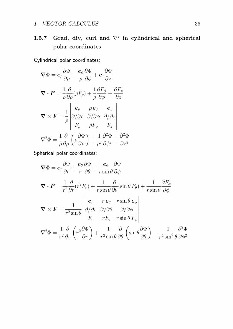
1.5.7 Grad, div, curl and ∇2 in cylindrical and spherical

polar coordinates

Cylindrical polar coordinates:

∇Φ = eρ∂Φ

∂ρ+

eϕρ

∂Φ

∂ϕ+ ez

∂Φ

∂z

∇ · F =1

ρ

∂

∂ρ(ρFρ) +

1

ρ

∂Fϕ

∂ϕ+∂Fz

∂z

∇× F =1

ρ

∣∣∣∣∣∣∣∣eρ ρ eϕ ez

∂/∂ρ ∂/∂ϕ ∂/∂z

Fρ ρFϕ Fz

∣∣∣∣∣∣∣∣∇2Φ =

1

ρ

∂

∂ρ

(ρ∂Φ

∂ρ

)+

1

ρ2∂2Φ

∂ϕ2+∂2Φ

∂z2

Spherical polar coordinates:

∇Φ = er∂Φ

∂r+

eθr

∂Φ

∂θ+

eϕr sin θ

∂Φ

∂ϕ

∇ · F =1

r2∂

∂r(r2Fr) +

1

r sin θ

∂

∂θ(sin θ Fθ) +

1

r sin θ

∂Fϕ

∂ϕ

∇× F =1

r2 sin θ

∣∣∣∣∣∣∣∣er r eθ r sin θ eϕ

∂/∂r ∂/∂θ ∂/∂ϕ

Fr rFθ r sin θ Fϕ

∣∣∣∣∣∣∣∣∇2Φ =

1

r2∂

∂r

(r2∂Φ

∂r

)+

1

r2 sin θ

∂

∂θ

(sin θ

∂Φ

∂θ

)+

1

r2 sin2 θ

∂2Φ

∂ϕ2

1 VECTOR CALCULUS 37

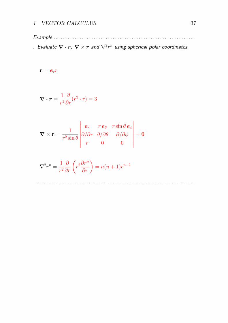
Example . . . . . . . . . . . . . . . . . . . . . . . . . . . . . . . . . . . . . . . . . . . . . . . . . . . . . . . . . . . .

▷ Evaluate ∇ · r, ∇× r and ∇2rn using spherical polar coordinates.

r = err

∇ · r =1

r2∂

∂r(r2 · r) = 3

∇× r =1

r2 sin θ

∣∣∣∣∣∣∣∣er r eθ r sin θ eϕ

∂/∂r ∂/∂θ ∂/∂ϕ

r 0 0

∣∣∣∣∣∣∣∣ = 0

∇2rn =1

r2∂

∂r

(r2∂rn

∂r

)= n(n+ 1)rn−2

. . . . . . . . . . . . . . . . . . . . . . . . . . . . . . . . . . . . . . . . . . . . . . . . . . . . . . . . . . . . . . . . . . . .

2 PARTIAL DIFFERENTIAL EQUATIONS 38

2 Partial differential equations

2.1 Motivation

The variation in space and time of scientific quantities is usually described

by differential equations. If the quantities depend on space and time, or

on more than one spatial coordinate, then the governing equations are

partial differential equations (PDEs).

Many of the most important PDEs are linear and classical methods of

analysis can be applied. The techniques developed for linear equations

are also useful in the study of nonlinear PDEs.

2.2 Linear PDEs of second order

2.2.1 Definition

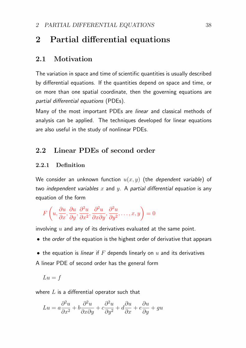
We consider an unknown function u(x, y) (the dependent variable) of

two independent variables x and y. A partial differential equation is any

equation of the form

F

(u,∂u

∂x,∂u

∂y,∂2u

∂x2,∂2u

∂x∂y,∂2u

∂y2, . . . , x, y

)= 0

involving u and any of its derivatives evaluated at the same point.

• the order of the equation is the highest order of derivative that appears

• the equation is linear if F depends linearly on u and its derivatives

A linear PDE of second order has the general form

Lu = f

where L is a differential operator such that

Lu = a∂2u

∂x2+ b

∂2u

∂x∂y+ c

∂2u

∂y2+ d

∂u

∂x+ e

∂u

∂y+ gu

2 PARTIAL DIFFERENTIAL EQUATIONS 39

where a, b, c, d, e, f, g are functions of x and y.

• if f = 0 the equation is said to be homogeneous

• if a, b, c, d, e, g are independent of x and y the equation is said to have

constant coefficients

These ideas can be generalized to more than two independent variables,

or to systems of PDEs with more than one dependent variable.

2.2.2 Principle of superposition

L defined above is an example of a linear operator :

L(αu) = αLu

and

L(u+ v) = Lu+ Lv

where u and v any functions of x and y, and α is any constant.

The principle of superposition:

• if u and v satisfy the homogeneous equation Lu = 0, then αu and

u+ v also satisfy the homogeneous equation

• similarly, any linear combination of solutions of the homogeneous equa-

tion is also a solution

• if the particular integral up satisfies the inhomogeneous equation Lu =

f and the complementary function uc satisfies the homogeneous equa-

tion Lu = 0, then up + uc also satisfies the inhomogeneous equation:

L(up + uc) = Lup + Luc = f + 0 = f

The same principle applies to any other type of linear equation (e.g. al-

gebraic, ordinary differential, integral).

2 PARTIAL DIFFERENTIAL EQUATIONS 40

2.2.3 Classic examples

Laplace’s equation:

∇2u = 0

Diffusion equation (heat equation):

∂u

∂t= λ∇2u, λ = diffusion coefficient (or diffusivity)

Wave equation:

∂2u

∂t2= c2∇2u, c = wave speed

All involve the vector-invariant operator ∇2, the form of which depends

on the number of active dimensions.

Inhomogeneous versions of these equations are also found. The inhomo-

geneous term usually represents a ‘source’ or ‘force’ that generates or

drives the quantity u.

2.3 Physical examples of occurrence

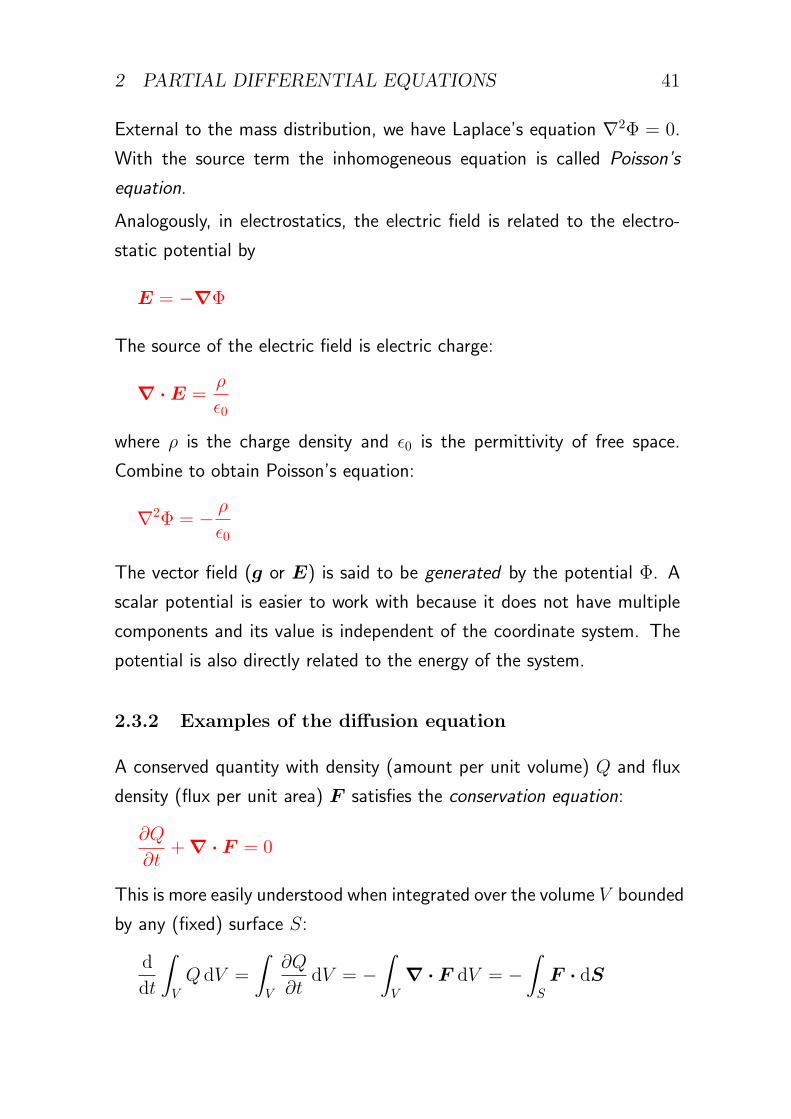
2.3.1 Examples of Laplace’s (or Poisson’s) equation

Gravitational acceleration is related to gravitational potential by

g = −∇Φ

The source (divergence) of the gravitational field is mass:

∇ · g = −4πGρ

where G is Newton’s constant and ρ is the mass density. Combine:

∇2Φ = 4πGρ

2 PARTIAL DIFFERENTIAL EQUATIONS 41

External to the mass distribution, we have Laplace’s equation ∇2Φ = 0.

With the source term the inhomogeneous equation is called Poisson’s

equation.

Analogously, in electrostatics, the electric field is related to the electro-

static potential by

E = −∇Φ

The source of the electric field is electric charge:

∇ ·E =ρ

ϵ0

where ρ is the charge density and ϵ0 is the permittivity of free space.

Combine to obtain Poisson’s equation:

∇2Φ = − ρ

ϵ0

The vector field (g or E) is said to be generated by the potential Φ. A

scalar potential is easier to work with because it does not have multiple

components and its value is independent of the coordinate system. The

potential is also directly related to the energy of the system.

2.3.2 Examples of the diffusion equation

A conserved quantity with density (amount per unit volume) Q and flux

density (flux per unit area) F satisfies the conservation equation:

∂Q

∂t+∇ · F = 0

This is more easily understood when integrated over the volume V bounded

by any (fixed) surface S:

d

dt

∫V

Q dV =

∫V

∂Q

∂tdV = −

∫V

∇ · F dV = −∫S

F · dS

2 PARTIAL DIFFERENTIAL EQUATIONS 42

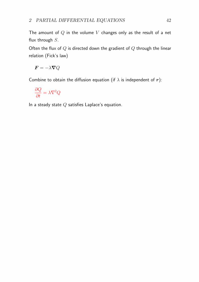
The amount of Q in the volume V changes only as the result of a net

flux through S.

Often the flux of Q is directed down the gradient of Q through the linear

relation (Fick’s law)

F = −λ∇Q

Combine to obtain the diffusion equation (if λ is independent of r):

∂Q

∂t= λ∇2Q

In a steady state Q satisfies Laplace’s equation.

2 PARTIAL DIFFERENTIAL EQUATIONS 43

Example . . . . . . . . . . . . . . . . . . . . . . . . . . . . . . . . . . . . . . . . . . . . . . . . . . . . . . . . . . . .

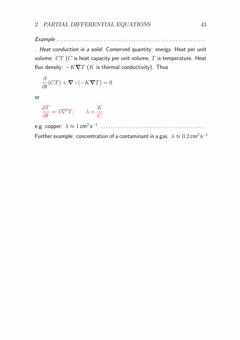
▷ Heat conduction in a solid. Conserved quantity: energy. Heat per unit

volume: CT (C is heat capacity per unit volume, T is temperature. Heat

flux density: −K∇T (K is thermal conductivity). Thus

∂

∂t(CT ) +∇ · (−K∇T ) = 0

or

∂T

∂t= λ∇2T, λ =

K

C

e.g. copper: λ ≈ 1 cm2 s−1 . . . . . . . . . . . . . . . . . . . . . . . . . . . . . . . . . . . . . . . . . .

Further example: concentration of a contaminant in a gas. λ ≈ 0.2 cm2 s−1

2 PARTIAL DIFFERENTIAL EQUATIONS 44

2.3.3 Examples of the wave equation

Waves on a string. The string has uniform mass per unit length ρ

and uniform tension T . The transverse displacement y(x, t) is small

(|∂y/∂x| ≪ 1) and satisfies Newton’s second law for an element δs of

the string:

(ρ δs)∂2y

∂t2= δFy ≈

∂Fy

∂xδx

Now,

Fy = T sin θ ≈ T tan θ ≈ T∂y

∂x, and also δs ≈ δx

where θ is the small angle between the x-axis and the tangent to the

string. Combine to obtain the one-dimensional wave equation

∂2y

∂t2= c2

∂2y

∂x2, c =

√T

ρ

e.g. violin (D-)string: T ≈ 40N, ρ ≈ 1 gm−1: c ≈ 200ms−1

Electromagnetic waves. Maxwell’s equations for the electromagnetic field

in a vacuum:

∇ ·E = 0

∇ ·B = 0

∇×E +∂B

∂t= 0

1

µ0∇×B − ϵ0

∂E

∂t= 0

2 PARTIAL DIFFERENTIAL EQUATIONS 45

where E is electric field, B is magnetic field, µ0 is the permeability of

free space and ϵ0 is the permittivity of free space. Eliminate E:

∂2B

∂t2= −∇× ∂E

∂t= − 1

µ0ϵ0∇× (∇×B)

Now use the identity ∇× (∇×B) = ∇(∇ ·B)−∇2B and Maxwell’s

equation ∇ ·B = 0 to obtain the (vector) wave equation

∂2B

∂t2= c2∇2B, c =

√1

µ0ϵ0

E obeys the same equation. c is the speed of light. c ≈ 3× 108ms−1

Further example: sound waves in a gas. c ≈ 300ms−1

2.3.4 Examples of other second-order linear PDEs

Schrodinger’s equation (quantum-mechanical wavefunction of a particle

of mass m in a potential V ):

iℏ∂ψ

∂t= − ℏ2

2m∇2ψ + V (r)ψ

Helmholtz equation (arises in wave problems):

∇2u+ k2u = 0

Klein–Gordon equation (arises in relativistic quantum mechanics):

∂2u

∂t2= c2(∇2u−m2u)

2.3.5 Examples of nonlinear PDEs

Burgers’ equation (describes shock waves):

∂u

∂t+ u

∂u

∂x= λ∇2u

2 PARTIAL DIFFERENTIAL EQUATIONS 46

Nonlinear Schrodinger equation (describes solitons, e.g. in optical fibre

communication):

i∂ψ

∂t= −∇2ψ − |ψ|2ψ

These equations require different methods of analysis.

2.4 Separation of variables (Cartesian coordinates)

2.4.1 Diffusion equation

We consider the one-dimensional diffusion equation (e.g. conduction of

heat along a metal bar):

∂u

∂t= λ

∂2u

∂x2

The bar could be considered finite (having two ends), semi-infinite (having

one end) or infinite (having no end). Typical boundary conditions at an

end are:

• u is specified (Dirichlet boundary condition)

• ∂u/∂x is specified (Neumann boundary condition)

If a boundary is removed to infinity, we usually require instead that u be

bounded (i.e. remain finite) as x → ±∞. This condition is needed to

eliminate unphysical solutions.

To determine the solution fully we also require initial conditions. For the

diffusion equation this means specifying u as a function of x at some

initial time (usually t = 0).

Try a solution in which the variables appear in separate factors:

u(x, t) = X(x)T (t)

Substitute this into the PDE:

X(x)T ′(t) = λX ′′(x)T (t)

2 PARTIAL DIFFERENTIAL EQUATIONS 47

(recall that a prime denotes differentiation of a function with respect to

its argument). Divide through by λXT to separate the variables:

T ′(t)

λT (t)=X ′′(x)

X(x)

The LHS depends only on t, while the RHS depends only on x. Both

must therefore equal a constant, which we call −k2 (for later conveniencehere – at this stage the constant could still be positive or negative). The

PDE is separated into two ordinary differential equations (ODEs)

T ′ + λk2T = 0

X ′′ + k2X = 0

with general solutions

T = A exp(−λk2t)

X = B sin(kx) + C cos(kx)

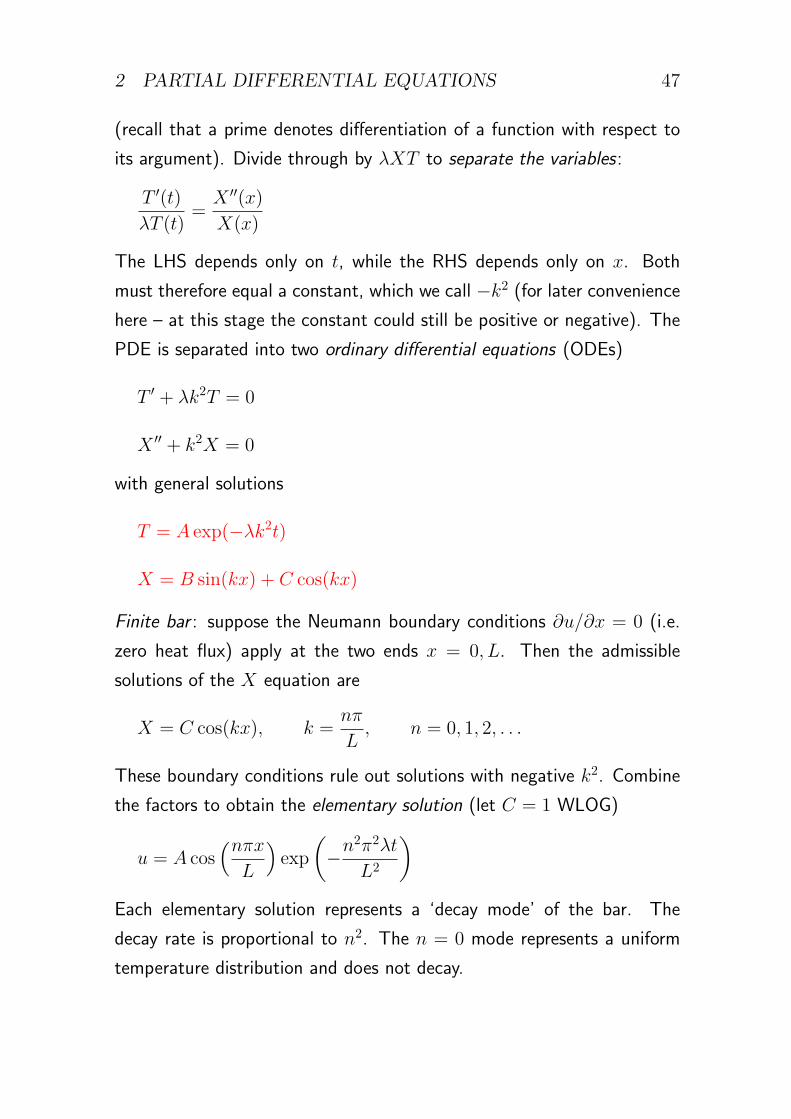
Finite bar : suppose the Neumann boundary conditions ∂u/∂x = 0 (i.e.

zero heat flux) apply at the two ends x = 0, L. Then the admissible

solutions of the X equation are

X = C cos(kx), k =nπ

L, n = 0, 1, 2, . . .

These boundary conditions rule out solutions with negative k2. Combine

the factors to obtain the elementary solution (let C = 1 WLOG)

u = A cos(nπxL

)exp

(−n

2π2λt

L2

)Each elementary solution represents a ‘decay mode’ of the bar. The

decay rate is proportional to n2. The n = 0 mode represents a uniform

temperature distribution and does not decay.

2 PARTIAL DIFFERENTIAL EQUATIONS 48

The principle of superposition allows us to construct a general solution as

a linear combination of elementary solutions:

u(x, t) =∞∑n=0

An cos(nπxL

)exp

(−n

2π2λt

L2

)The coefficients An can be determined from the initial conditions. If the

temperature at time t = 0 is specified, then

u(x, 0) =∞∑n=0

An cos(nπxL

)is known. The coefficients An are just the Fourier coefficients of the initial

temperature distribution.

Semi-infinite bar : The solution X ∝ cos(kx) is valid for any real value

of k so that u is bounded as x → ∞. We may assume k ⩾ 0 WLOG.

The solution decays in time unless k = 0. The general solution is a linear

combination in the form of an integral:

u =

∫ ∞

0

A(k) cos(kx) exp(−λk2t) dk

This is an example of a Fourier integral, studied in section 4.

Notes:

• separation of variables doesn’t work for all linear equations, by any

means, but it does for some of the most important examples

• it is not supposed to be obvious that the most general solution can be

written as a linear combination of separated solutions

2.4.2 Wave equation (example)

∂2u

∂t2= c2

∂2u

∂x2, 0 < x < L

Boundary conditions:

u = 0 at x = 0, L

2 PARTIAL DIFFERENTIAL EQUATIONS 49

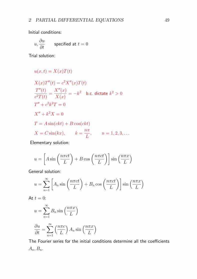
Initial conditions:

u,∂u

∂tspecified at t = 0

Trial solution:

u(x, t) = X(x)T (t)

X(x)T ′′(t) = c2X ′′(x)T (t)

T ′′(t)

c2T (t)=X ′′(x)

X(x)= −k2 b.c. dictate k2 > 0

T ′′ + c2k2T = 0

X ′′ + k2X = 0

T = A sin(ckt) +B cos(ckt)

X = C sin(kx), k =nπ

L, n = 1, 2, 3, . . .

Elementary solution:

u =

[A sin

(nπct

L

)+B cos

(nπct

L

)]sin

(nπxL

)General solution:

u =∞∑n=1

[An sin

(nπct

L

)+Bn cos

(nπct

L

)]sin

(nπxL

)At t = 0:

u =∞∑n=1

Bn sin(nπxL

)∂u

∂t=

∞∑n=1

(nπcL

)An sin

(nπxL

)The Fourier series for the initial conditions determine all the coefficients

An, Bn.

2 PARTIAL DIFFERENTIAL EQUATIONS 50

2.4.3 Helmholtz equation (example)

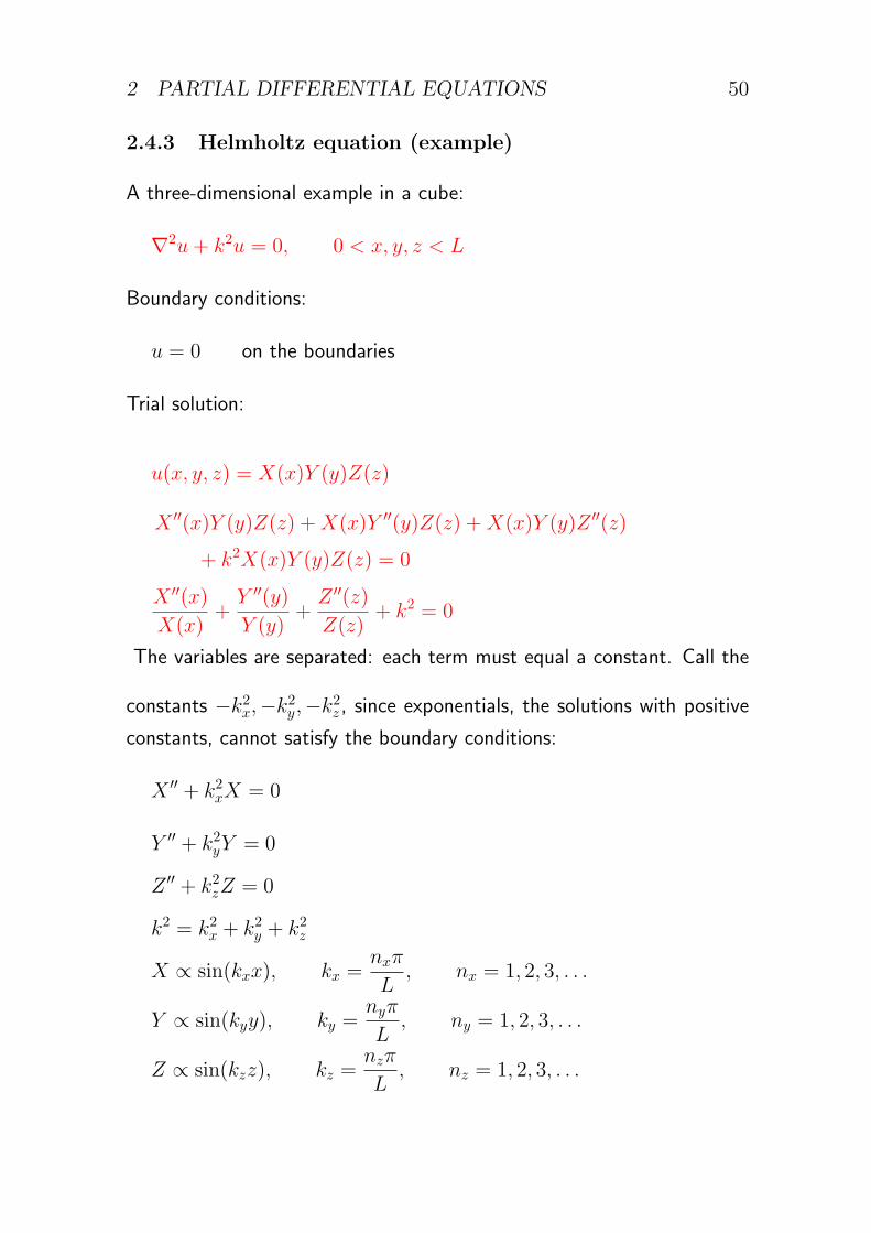
A three-dimensional example in a cube:

∇2u+ k2u = 0, 0 < x, y, z < L

Boundary conditions:

u = 0 on the boundaries

Trial solution:

u(x, y, z) = X(x)Y (y)Z(z)

X ′′(x)Y (y)Z(z) +X(x)Y ′′(y)Z(z) +X(x)Y (y)Z ′′(z)

+ k2X(x)Y (y)Z(z) = 0

X ′′(x)

X(x)+Y ′′(y)

Y (y)+Z ′′(z)

Z(z)+ k2 = 0

The variables are separated: each term must equal a constant. Call the

constants −k2x,−k2y,−k2z , since exponentials, the solutions with positive

constants, cannot satisfy the boundary conditions:

X ′′ + k2xX = 0

Y ′′ + k2yY = 0

Z ′′ + k2zZ = 0

k2 = k2x + k2y + k2z

X ∝ sin(kxx), kx =nxπ

L, nx = 1, 2, 3, . . .

Y ∝ sin(kyy), ky =nyπ

L, ny = 1, 2, 3, . . .

Z ∝ sin(kzz), kz =nzπ

L, nz = 1, 2, 3, . . .

2 PARTIAL DIFFERENTIAL EQUATIONS 51

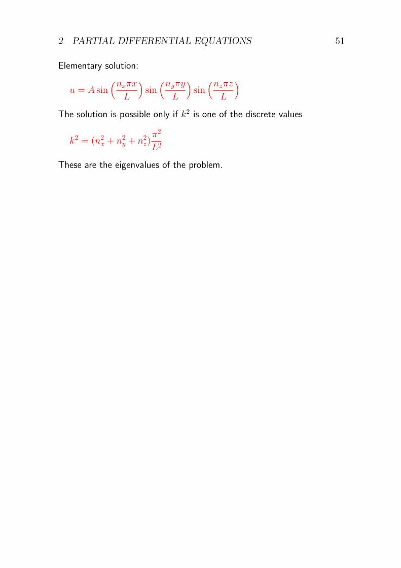
Elementary solution:

u = A sin(nxπx

L

)sin

(nyπyL

)sin

(nzπzL

)The solution is possible only if k2 is one of the discrete values

k2 = (n2x + n2y + n2z)π2

L2

These are the eigenvalues of the problem.

3 GREEN’S FUNCTIONS 52

3 Green’s functions

3.1 Impulses and the delta function

3.1.1 Physical motivation

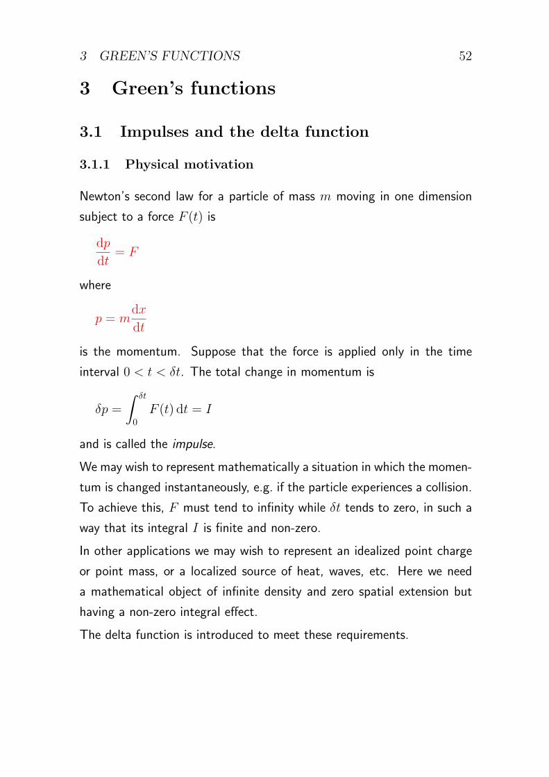
Newton’s second law for a particle of mass m moving in one dimension

subject to a force F (t) is

dp

dt= F

where

p = mdx

dt

is the momentum. Suppose that the force is applied only in the time

interval 0 < t < δt. The total change in momentum is

δp =

∫ δt

0

F (t) dt = I

and is called the impulse.

We may wish to represent mathematically a situation in which the momen-

tum is changed instantaneously, e.g. if the particle experiences a collision.

To achieve this, F must tend to infinity while δt tends to zero, in such a

way that its integral I is finite and non-zero.

In other applications we may wish to represent an idealized point charge

or point mass, or a localized source of heat, waves, etc. Here we need

a mathematical object of infinite density and zero spatial extension but

having a non-zero integral effect.

The delta function is introduced to meet these requirements.

3 GREEN’S FUNCTIONS 53

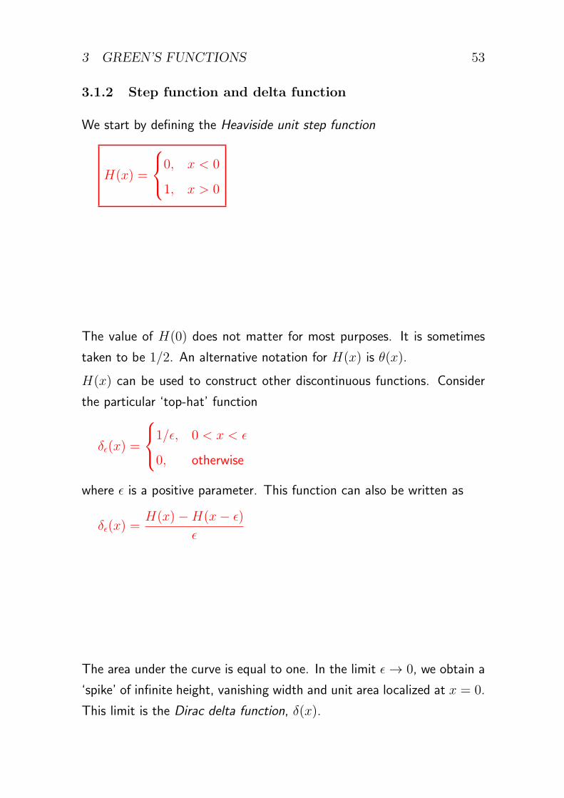
3.1.2 Step function and delta function

We start by defining the Heaviside unit step function

H(x) =

0, x < 0

1, x > 0

The value of H(0) does not matter for most purposes. It is sometimes

taken to be 1/2. An alternative notation for H(x) is θ(x).

H(x) can be used to construct other discontinuous functions. Consider

the particular ‘top-hat’ function

δϵ(x) =

1/ϵ, 0 < x < ϵ

0, otherwise

where ϵ is a positive parameter. This function can also be written as

δϵ(x) =H(x)−H(x− ϵ)

ϵ

The area under the curve is equal to one. In the limit ϵ→ 0, we obtain a

‘spike’ of infinite height, vanishing width and unit area localized at x = 0.

This limit is the Dirac delta function, δ(x).

3 GREEN’S FUNCTIONS 54

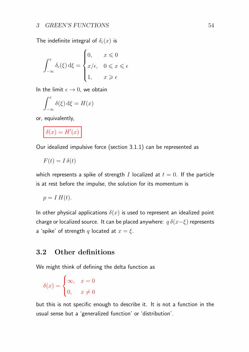
The indefinite integral of δϵ(x) is

∫ x

−∞δϵ(ξ) dξ =

0, x ⩽ 0

x/ϵ, 0 ⩽ x ⩽ ϵ

1, x ⩾ ϵ

In the limit ϵ→ 0, we obtain∫ x

−∞δ(ξ) dξ = H(x)

or, equivalently,

δ(x) = H ′(x)

Our idealized impulsive force (section 3.1.1) can be represented as

F (t) = I δ(t)

which represents a spike of strength I localized at t = 0. If the particle

is at rest before the impulse, the solution for its momentum is

p = I H(t).

In other physical applications δ(x) is used to represent an idealized point

charge or localized source. It can be placed anywhere: q δ(x−ξ) representsa ‘spike’ of strength q located at x = ξ.

3.2 Other definitions

We might think of defining the delta function as

δ(x) =

∞, x = 0

0, x = 0

but this is not specific enough to describe it. It is not a function in the

usual sense but a ‘generalized function’ or ‘distribution’.

3 GREEN’S FUNCTIONS 55

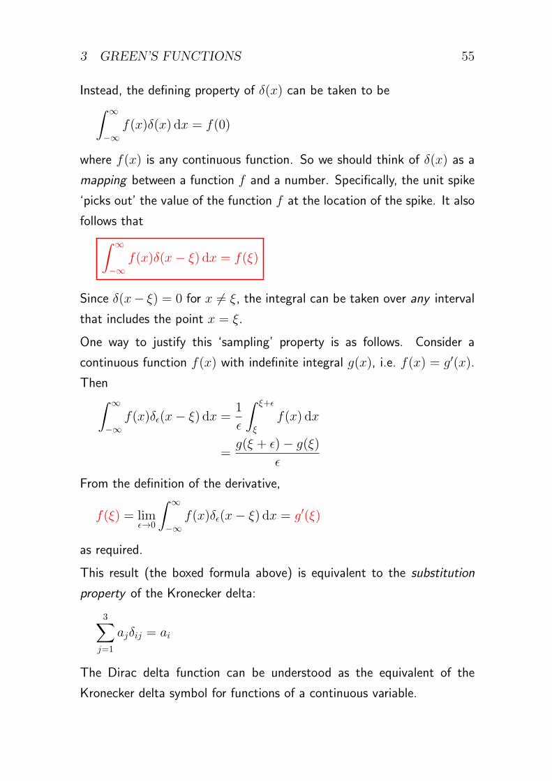
Instead, the defining property of δ(x) can be taken to be∫ ∞

−∞f(x)δ(x) dx = f(0)

where f(x) is any continuous function. So we should think of δ(x) as a

mapping between a function f and a number. Specifically, the unit spike

‘picks out’ the value of the function f at the location of the spike. It also

follows that∫ ∞

−∞f(x)δ(x− ξ) dx = f(ξ)

Since δ(x− ξ) = 0 for x = ξ, the integral can be taken over any interval

that includes the point x = ξ.

One way to justify this ‘sampling’ property is as follows. Consider a

continuous function f(x) with indefinite integral g(x), i.e. f(x) = g′(x).

Then∫ ∞

−∞f(x)δϵ(x− ξ) dx =

1

ϵ

∫ ξ+ϵ

ξ

f(x) dx

=g(ξ + ϵ)− g(ξ)

ϵ

From the definition of the derivative,

f(ξ) = limϵ→0

∫ ∞

−∞f(x)δϵ(x− ξ) dx = g′(ξ)

as required.

This result (the boxed formula above) is equivalent to the substitution

property of the Kronecker delta:

3∑j=1

ajδij = ai

The Dirac delta function can be understood as the equivalent of the

Kronecker delta symbol for functions of a continuous variable.

3 GREEN’S FUNCTIONS 56

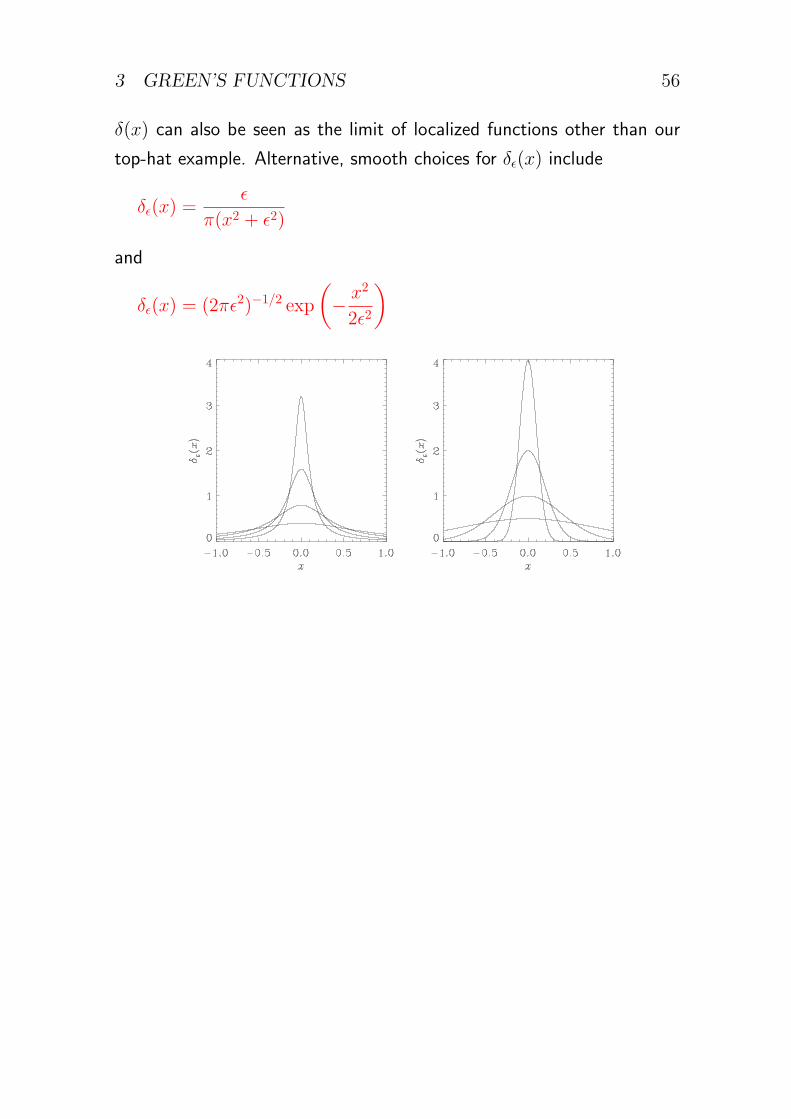
δ(x) can also be seen as the limit of localized functions other than our

top-hat example. Alternative, smooth choices for δϵ(x) include

δϵ(x) =ϵ

π(x2 + ϵ2)

and

δϵ(x) = (2πϵ2)−1/2 exp

(− x2

2ϵ2

)

3 GREEN’S FUNCTIONS 57

3.3 More on generalized functions

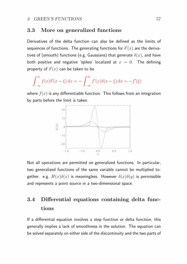
Derivatives of the delta function can also be defined as the limits of

sequences of functions. The generating functions for δ′(x) are the deriva-

tives of (smooth) functions (e.g. Gaussians) that generate δ(x), and have

both positive and negative ‘spikes’ localized at x = 0. The defining

property of δ′(x) can be taken to be∫ ∞

−∞f(x)δ′(x− ξ) dx = −

∫ ∞

−∞f ′(x)δ(x− ξ) dx = −f ′(ξ)

where f(x) is any differentiable function. This follows from an integration

by parts before the limit is taken.

Not all operations are permitted on generalized functions. In particular,

two generalized functions of the same variable cannot be multiplied to-

gether. e.g. H(x)δ(x) is meaningless. However δ(x)δ(y) is permissible

and represents a point source in a two-dimensional space.

3.4 Differential equations containing delta func-

tions

If a differential equation involves a step function or delta function, this

generally implies a lack of smoothness in the solution. The equation can

be solved separately on either side of the discontinuity and the two parts of

3 GREEN’S FUNCTIONS 58

the solution connected by applying the appropriate matching conditions.

Consider, as an example, the linear second-order ODE

d2y

dx2+ y = δ(x) (1)

If x represents time, this equation could represent the behaviour of a

simple harmonic oscillator in response to an impulsive force.

In each of the regions x < 0 and x > 0 separately, the right-hand side

vanishes and the general solution is a linear combination of cosx and

sinx. We may write

y =

A cosx+B sinx, x < 0

C cosx+D sinx, x > 0

Since the general solution of a second-order ODE should contain only two

arbitrary constants, it must be possible to relate C and D to A and B.

What is the nature of the non-smoothness in y?

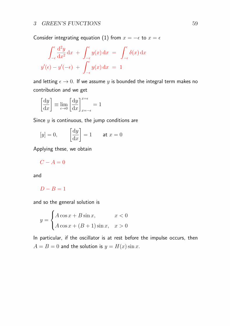
3 GREEN’S FUNCTIONS 59

Consider integrating equation (1) from x = −ϵ to x = ϵ∫ ϵ

−ϵ

d2y

dx2dx +

∫ ϵ

−ϵ

y(x) dx =

∫ ϵ

−ϵ

δ(x) dx

y′(ϵ)− y′(−ϵ) +

∫ ϵ

−ϵ

y(x) dx = 1

and letting ϵ→ 0. If we assume y is bounded the integral term makes no

contribution and we get[dy

dx

]≡ lim

ϵ→0

[dy

dx

]x=ϵ

x=−ϵ

= 1

Since y is continuous, the jump conditions are

[y] = 0,

[dy

dx

]= 1 at x = 0

Applying these, we obtain

C − A = 0

and

D −B = 1

and so the general solution is

y =

A cosx+B sinx, x < 0

A cosx+ (B + 1) sinx, x > 0

In particular, if the oscillator is at rest before the impulse occurs, then

A = B = 0 and the solution is y = H(x) sin x.

3 GREEN’S FUNCTIONS 60

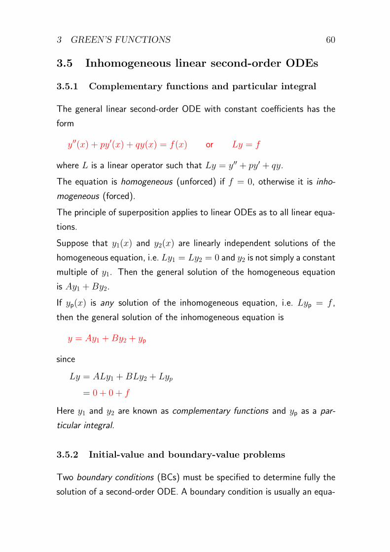
3.5 Inhomogeneous linear second-order ODEs

3.5.1 Complementary functions and particular integral

The general linear second-order ODE with constant coefficients has the

form

y′′(x) + py′(x) + qy(x) = f(x) or Ly = f

where L is a linear operator such that Ly = y′′ + py′ + qy.

The equation is homogeneous (unforced) if f = 0, otherwise it is inho-

mogeneous (forced).

The principle of superposition applies to linear ODEs as to all linear equa-

tions.

Suppose that y1(x) and y2(x) are linearly independent solutions of the

homogeneous equation, i.e. Ly1 = Ly2 = 0 and y2 is not simply a constant

multiple of y1. Then the general solution of the homogeneous equation

is Ay1 +By2.

If yp(x) is any solution of the inhomogeneous equation, i.e. Lyp = f ,

then the general solution of the inhomogeneous equation is

y = Ay1 +By2 + yp

since

Ly = ALy1 +BLy2 + Lyp

= 0 + 0 + f

Here y1 and y2 are known as complementary functions and yp as a par-

ticular integral.

3.5.2 Initial-value and boundary-value problems

Two boundary conditions (BCs) must be specified to determine fully the

solution of a second-order ODE. A boundary condition is usually an equa-

3 GREEN’S FUNCTIONS 61

tion relating the values of y and y′ at one point. (The ODE allows y′′

and higher derivatives to be expressed in terms of y and y′.)

The general form of a linear BC at a point x = a is

α1y′(a) + α2y(a) = α3

where α1, α2, α3 are constants and α1, α2 are not both zero. If α3 = 0

the BC is homogeneous.

If both BCs are specified at the same point we have an initial-value prob-

lem, e.g. to solve

md2x

dt2= F (t) for t ⩾ 0 subject to x =

dx

dt= 0 at t = 0

If the BCs are specified at different points we have a two-point boundary-

value problem, e.g. to solve

y′′(x) + y(x) = f(x) for a ⩽ x ⩽ b subject to y(a) = y(b) = 0

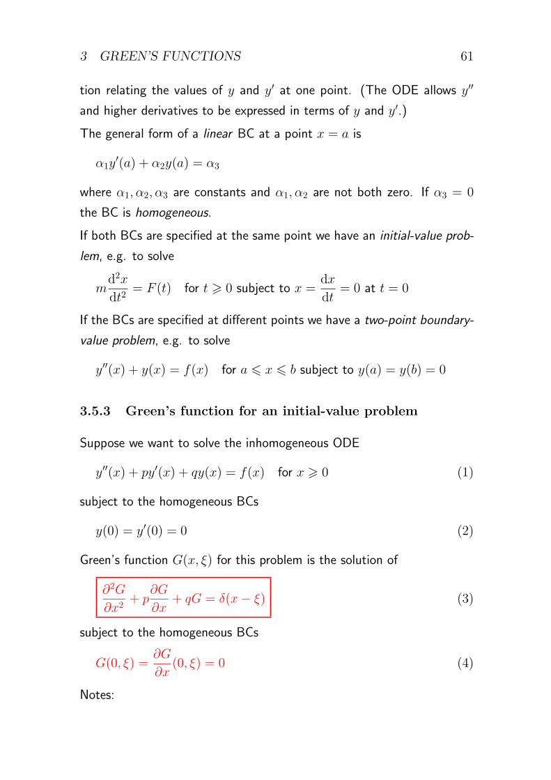
3.5.3 Green’s function for an initial-value problem

Suppose we want to solve the inhomogeneous ODE

y′′(x) + py′(x) + qy(x) = f(x) for x ⩾ 0 (1)

subject to the homogeneous BCs

y(0) = y′(0) = 0 (2)

Green’s function G(x, ξ) for this problem is the solution of

∂2G

∂x2+ p

∂G

∂x+ qG = δ(x− ξ) (3)

subject to the homogeneous BCs

G(0, ξ) =∂G

∂x(0, ξ) = 0 (4)

Notes:

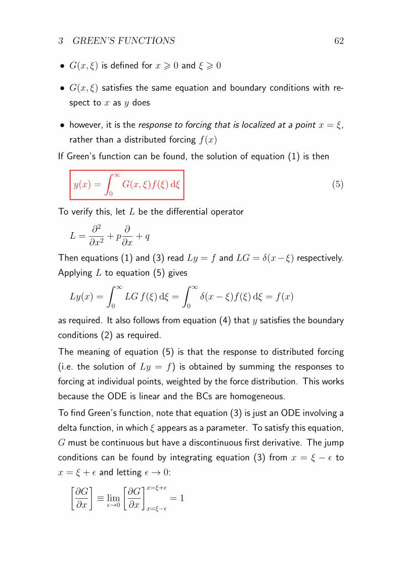
3 GREEN’S FUNCTIONS 62

• G(x, ξ) is defined for x ⩾ 0 and ξ ⩾ 0

• G(x, ξ) satisfies the same equation and boundary conditions with re-

spect to x as y does

• however, it is the response to forcing that is localized at a point x = ξ,

rather than a distributed forcing f(x)

If Green’s function can be found, the solution of equation (1) is then

y(x) =

∫ ∞

0

G(x, ξ)f(ξ) dξ (5)

To verify this, let L be the differential operator

L =∂2

∂x2+ p

∂

∂x+ q

Then equations (1) and (3) read Ly = f and LG = δ(x−ξ) respectively.Applying L to equation (5) gives

Ly(x) =

∫ ∞

0

LGf(ξ) dξ =

∫ ∞

0

δ(x− ξ)f(ξ) dξ = f(x)

as required. It also follows from equation (4) that y satisfies the boundary

conditions (2) as required.

The meaning of equation (5) is that the response to distributed forcing

(i.e. the solution of Ly = f) is obtained by summing the responses to

forcing at individual points, weighted by the force distribution. This works

because the ODE is linear and the BCs are homogeneous.

To find Green’s function, note that equation (3) is just an ODE involving a

delta function, in which ξ appears as a parameter. To satisfy this equation,

G must be continuous but have a discontinuous first derivative. The jump

conditions can be found by integrating equation (3) from x = ξ − ϵ to

x = ξ + ϵ and letting ϵ→ 0:[∂G

∂x

]≡ lim

ϵ→0

[∂G

∂x

]x=ξ+ϵ

x=ξ−ϵ

= 1

3 GREEN’S FUNCTIONS 63

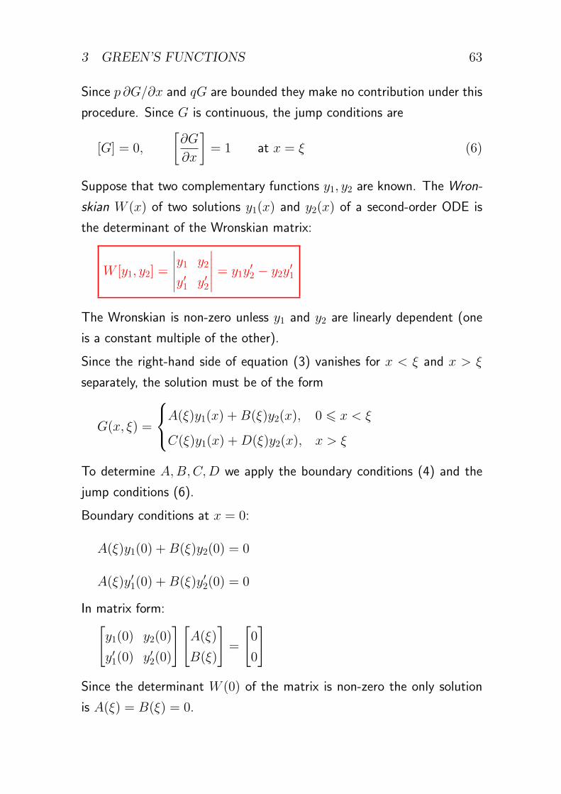
Since p ∂G/∂x and qG are bounded they make no contribution under this

procedure. Since G is continuous, the jump conditions are

[G] = 0,

[∂G

∂x

]= 1 at x = ξ (6)

Suppose that two complementary functions y1, y2 are known. The Wron-

skian W (x) of two solutions y1(x) and y2(x) of a second-order ODE is

the determinant of the Wronskian matrix:

W [y1, y2] =

∣∣∣∣∣y1 y2

y′1 y′2

∣∣∣∣∣ = y1y′2 − y2y

′1

The Wronskian is non-zero unless y1 and y2 are linearly dependent (one

is a constant multiple of the other).

Since the right-hand side of equation (3) vanishes for x < ξ and x > ξ

separately, the solution must be of the form

G(x, ξ) =

A(ξ)y1(x) +B(ξ)y2(x), 0 ⩽ x < ξ

C(ξ)y1(x) +D(ξ)y2(x), x > ξ

To determine A,B,C,D we apply the boundary conditions (4) and the

jump conditions (6).

Boundary conditions at x = 0:

A(ξ)y1(0) +B(ξ)y2(0) = 0

A(ξ)y′1(0) +B(ξ)y′2(0) = 0

In matrix form:[y1(0) y2(0)

y′1(0) y′2(0)

][A(ξ)

B(ξ)

]=

[0

0

]

Since the determinant W (0) of the matrix is non-zero the only solution

is A(ξ) = B(ξ) = 0.

3 GREEN’S FUNCTIONS 64

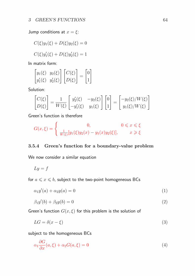
Jump conditions at x = ξ:

C(ξ)y1(ξ) +D(ξ)y2(ξ) = 0

C(ξ)y′1(ξ) +D(ξ)y′2(ξ) = 1

In matrix form:[y1(ξ) y2(ξ)

y′1(ξ) y′2(ξ)

][C(ξ)

D(ξ)

]=

[0

1

]Solution:[

C(ξ)

D(ξ)

]=

1

W (ξ)

[y′2(ξ) −y2(ξ)−y′1(ξ) y1(ξ)

][0

1

]=

[−y2(ξ)/W (ξ)

y1(ξ)/W (ξ)

]Green’s function is therefore

G(x, ξ) =

{0, 0 ⩽ x ⩽ ξ

1W (ξ) [y1(ξ)y2(x)− y1(x)y2(ξ)], x ⩾ ξ

3.5.4 Green’s function for a boundary-value problem

We now consider a similar equation

Ly = f

for a ⩽ x ⩽ b, subject to the two-point homogeneous BCs

α1y′(a) + α2y(a) = 0 (1)

β1y′(b) + β2y(b) = 0 (2)

Green’s function G(x, ξ) for this problem is the solution of

LG = δ(x− ξ) (3)

subject to the homogeneous BCs

α1∂G

∂x(a, ξ) + α2G(a, ξ) = 0 (4)

3 GREEN’S FUNCTIONS 65

β1∂G

∂x(b, ξ) + β2G(b, ξ) = 0 (5)

and is defined for a ⩽ x ⩽ b and a ⩽ ξ ⩽ b.

By a similar argument, the solution of Ly = f subject to the BCs (1) and

(2) is then

y(x) =

∫ b

a

G(x, ξ)f(ξ) dξ

We find Green’s function by a similar method. Let ya(x) be a com-

plementary function satisfying the left-hand BC (1), and let yb(x) be a

complementary function satisfying the right-hand BC (2). (These can

always be found.) Since the right-hand side of equation (3) vanishes for

x < ξ and x > ξ separately, the solution must be of the form

G(x, ξ) =

A(ξ)ya(x), a ⩽ x ⩽ ξ

B(ξ)yb(x), ξ ⩽ x ⩽ b

satisfying the BCs (4) and (5). To determine A,B we apply the jump

conditions [G] = 0 and [∂G/∂x] = 1 at x = ξ:

B(ξ)yb(ξ)− A(ξ)ya(ξ) = 0

B(ξ)y′b(ξ)− A(ξ)y′a(ξ) = 1

In matrix form:[ya(ξ) yb(ξ)

y′a(ξ) y′b(ξ)

][−A(ξ)B(ξ)

]=

[0

1

]Solution:[

−A(ξ)B(ξ)

]=

1

W (ξ)

[y′b(ξ) −yb(ξ)−y′a(ξ) ya(ξ)

][0

1

]=

[−yb(ξ)/W (ξ)

ya(ξ)/W (ξ)

]Green’s function is therefore

G(x, ξ) =

1W (ξ) [ya(x)yb(ξ)], a ⩽ x ⩽ ξ

1W (ξ) [ya(ξ)yb(x)], ξ ⩽ x ⩽ b

3 GREEN’S FUNCTIONS 66

This method fails if the Wronskian W [ya, yb] vanishes. This happens if

ya is proportional to yb, i.e. if there is a complementary function that

happens to satisfy both homogeneous BCs. In this (exceptional) case the

equation Ly = f may not have a solution satisfying the BCs; if it does,

the solution will not be unique.

3.5.5 Examples of Green’s function

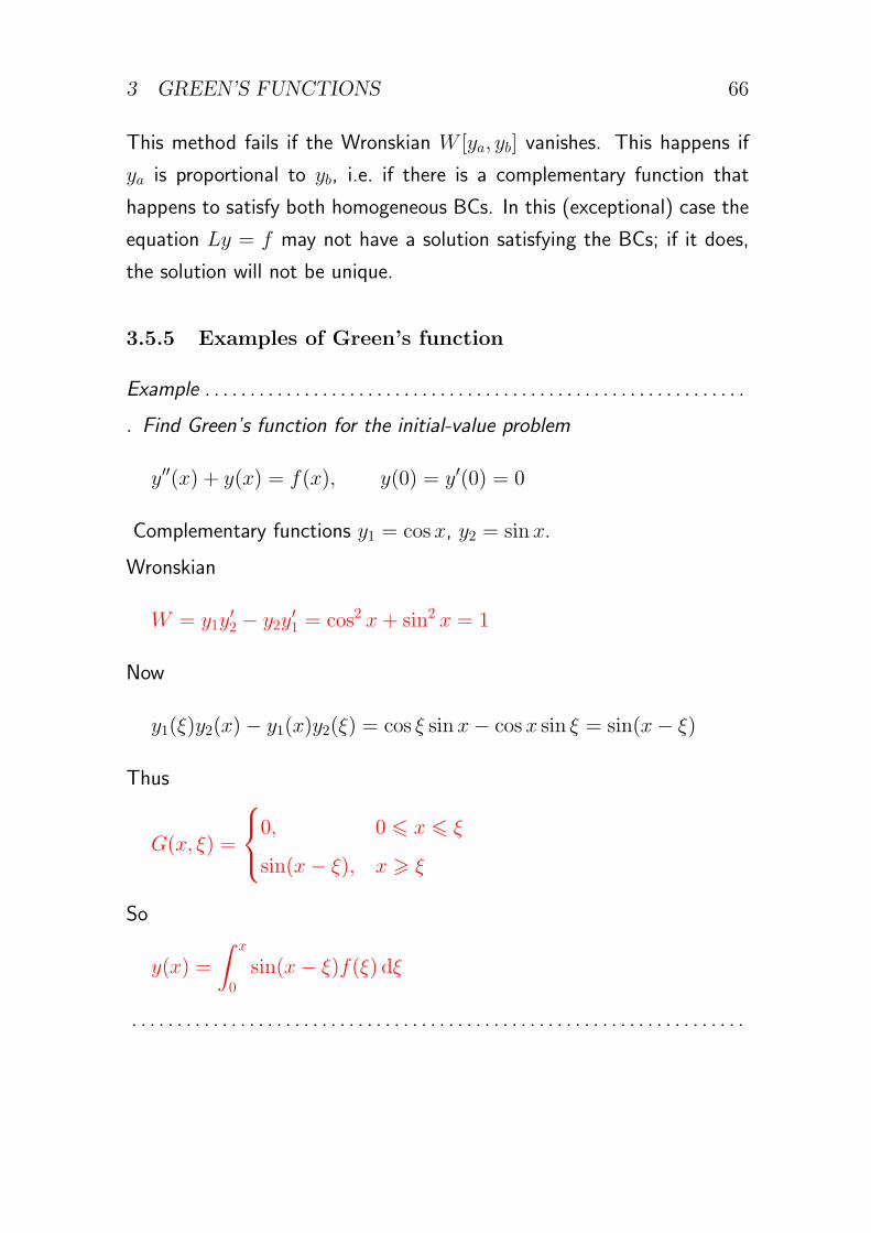
Example . . . . . . . . . . . . . . . . . . . . . . . . . . . . . . . . . . . . . . . . . . . . . . . . . . . . . . . . . . . .

▷ Find Green’s function for the initial-value problem

y′′(x) + y(x) = f(x), y(0) = y′(0) = 0

Complementary functions y1 = cos x, y2 = sin x.

Wronskian

W = y1y′2 − y2y

′1 = cos2 x+ sin2 x = 1

Now

y1(ξ)y2(x)− y1(x)y2(ξ) = cos ξ sinx− cosx sin ξ = sin(x− ξ)

Thus

G(x, ξ) =

0, 0 ⩽ x ⩽ ξ

sin(x− ξ), x ⩾ ξ

So

y(x) =

∫ x

0

sin(x− ξ)f(ξ) dξ

. . . . . . . . . . . . . . . . . . . . . . . . . . . . . . . . . . . . . . . . . . . . . . . . . . . . . . . . . . . . . . . . . . . .

3 GREEN’S FUNCTIONS 67

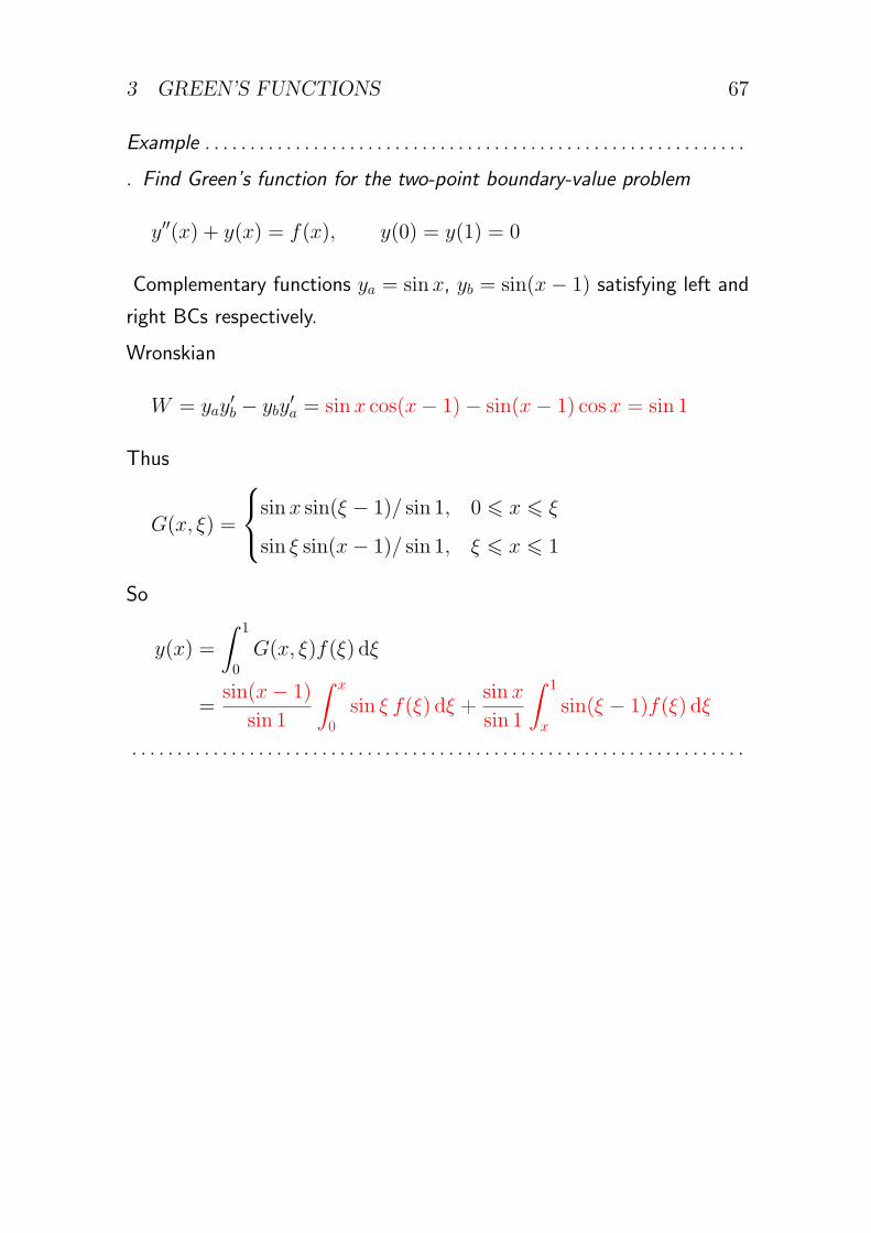
Example . . . . . . . . . . . . . . . . . . . . . . . . . . . . . . . . . . . . . . . . . . . . . . . . . . . . . . . . . . . .

▷ Find Green’s function for the two-point boundary-value problem

y′′(x) + y(x) = f(x), y(0) = y(1) = 0

Complementary functions ya = sin x, yb = sin(x− 1) satisfying left and

right BCs respectively.

Wronskian

W = yay′b − yby

′a = sinx cos(x− 1)− sin(x− 1) cosx = sin 1

Thus

G(x, ξ) =

sinx sin(ξ − 1)/ sin 1, 0 ⩽ x ⩽ ξ

sin ξ sin(x− 1)/ sin 1, ξ ⩽ x ⩽ 1

So

y(x) =

∫ 1

0

G(x, ξ)f(ξ) dξ

=sin(x− 1)

sin 1

∫ x

0

sin ξ f(ξ) dξ +sinx

sin 1

∫ 1

x

sin(ξ − 1)f(ξ) dξ

. . . . . . . . . . . . . . . . . . . . . . . . . . . . . . . . . . . . . . . . . . . . . . . . . . . . . . . . . . . . . . . . . . . .

3 GREEN’S FUNCTIONS 68

3.6 Unlectured remarks

1. Note that the solution y to a 2nd order differential equation of the

form Ly(x) = δ(x−x0) is continuous because of the properties of the

Dirac δ-function, specifically because its integral is finite (assuming the

limits of integration include x0).

2. So far we only considered problems with homogeneous boundary condi-

tions. One can also use Green’s functions to solve problems with inho-

mogeneous boundary conditions. The trick is to solve the homogenous

equation Lyp = 0 for a function yp which satisfies the inhomoge-

nous boundary condtions. Then solve the inhomogeneous equation

Lyg = f , perhaps using the Green’s function method discussed in this

chapter, imposing homogenous boundary conditions on yg. Then lin-

earity means that yp + yg satisfies the inhomogenous equation with

inhomogenous boundary conditions.

4 THE FOURIER TRANSFORM 69

4 The Fourier transform

4.1 Motivation

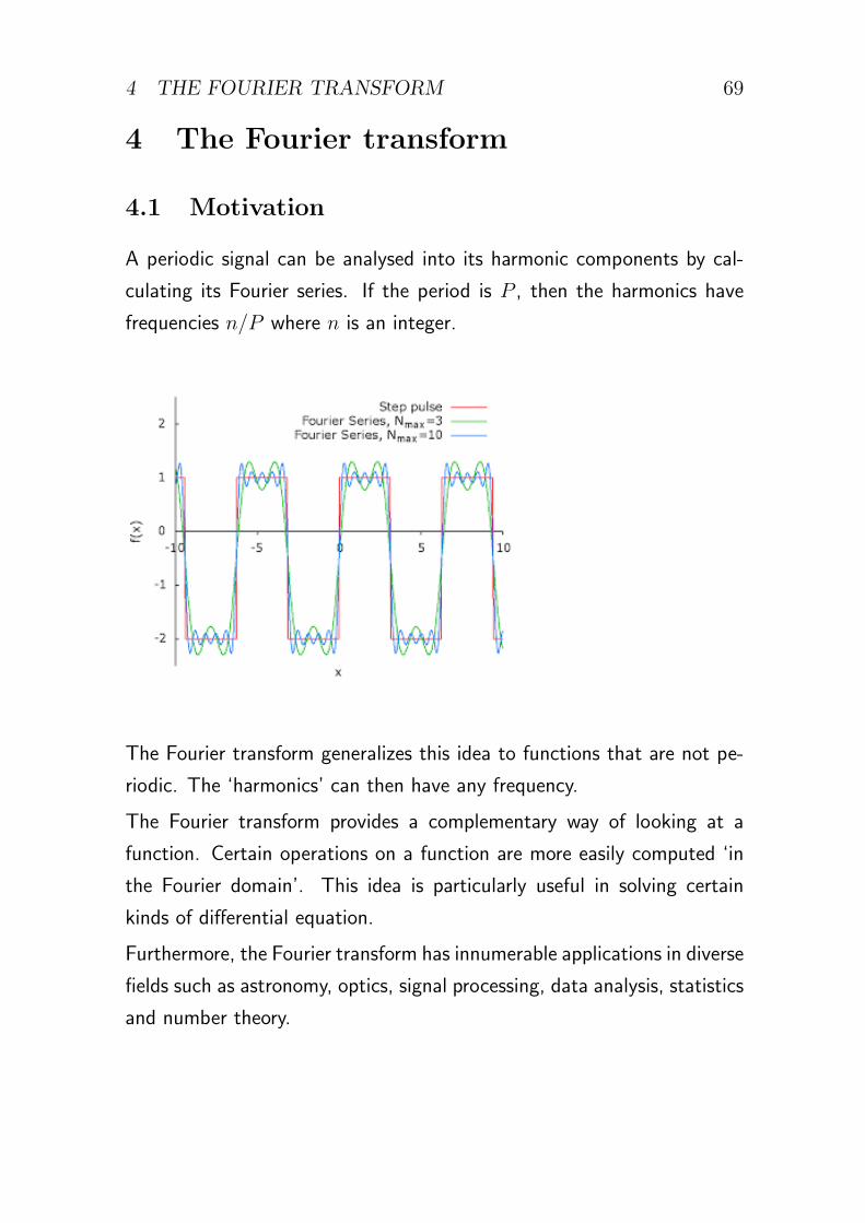
A periodic signal can be analysed into its harmonic components by cal-

culating its Fourier series. If the period is P , then the harmonics have

frequencies n/P where n is an integer.

The Fourier transform generalizes this idea to functions that are not pe-

riodic. The ‘harmonics’ can then have any frequency.

The Fourier transform provides a complementary way of looking at a

function. Certain operations on a function are more easily computed ‘in

the Fourier domain’. This idea is particularly useful in solving certain

kinds of differential equation.

Furthermore, the Fourier transform has innumerable applications in diverse

fields such as astronomy, optics, signal processing, data analysis, statistics

and number theory.

4 THE FOURIER TRANSFORM 70

4.2 Relation to Fourier series

A function f(x) has period P if f(x + P ) = f(x) for all x. It can then

be written as a Fourier series

f(x) =1

2a0 +

∞∑n=1

an cos(knx) +∞∑n=1

bn sin(knx)

where

kn =2πn

P

is the wavenumber of the nth harmonic.

Such a series is also used to write any function that is defined only on an

interval of length P , e.g. −P/2 < x < P/2. The Fourier series gives the

extension of the function by periodic repetition.

The Fourier coefficients are found from

an =2

P

∫ P/2

−P/2

f(x) cos(knx) dx

bn =2

P

∫ P/2

−P/2

f(x) sin(knx) dx

Define

cn =

(a−n + ib−n)/2, n < 0

a0/2, n = 0

(an − ibn)/2, n > 0

4 THE FOURIER TRANSFORM 71

Then the same result can be expressed more simply and compactly in the

notation of the complex Fourier series

f(x) =∞∑

n=−∞cn e

iknx

where, after multiplying the preceding equation by exp(−ikmx) and inte-

grating we find (recall km = 2πm/P )

cm =1

P

∫ P/2

−P/2

f(x) e−ikmx dx

This expression for cm (equivalently cn, relabellingm→ n) can be verified

using the orthogonality relation

1

P

∫ P/2

−P/2

ei(kn−km)x dx = δmn

which follows from an elementary integration.

To approach the Fourier transform, let P → ∞ so that the function is

defined on the entire real line without any periodicity. The wavenumbers

kn = 2πn/P are replaced by a continuous variable k, because

∆k = kn+1 − kn =2π

P→ 0 .

Consider the definition of the Fourier series

f(x) =∞∑

n=−∞cn e

iknx =1

2π

∞∑n=−∞

Pcn eiknx∆k, (1)

In the limit of P → ∞ this looks like the Riemann approximation to an

integral over k.

4 THE FOURIER TRANSFORM 72

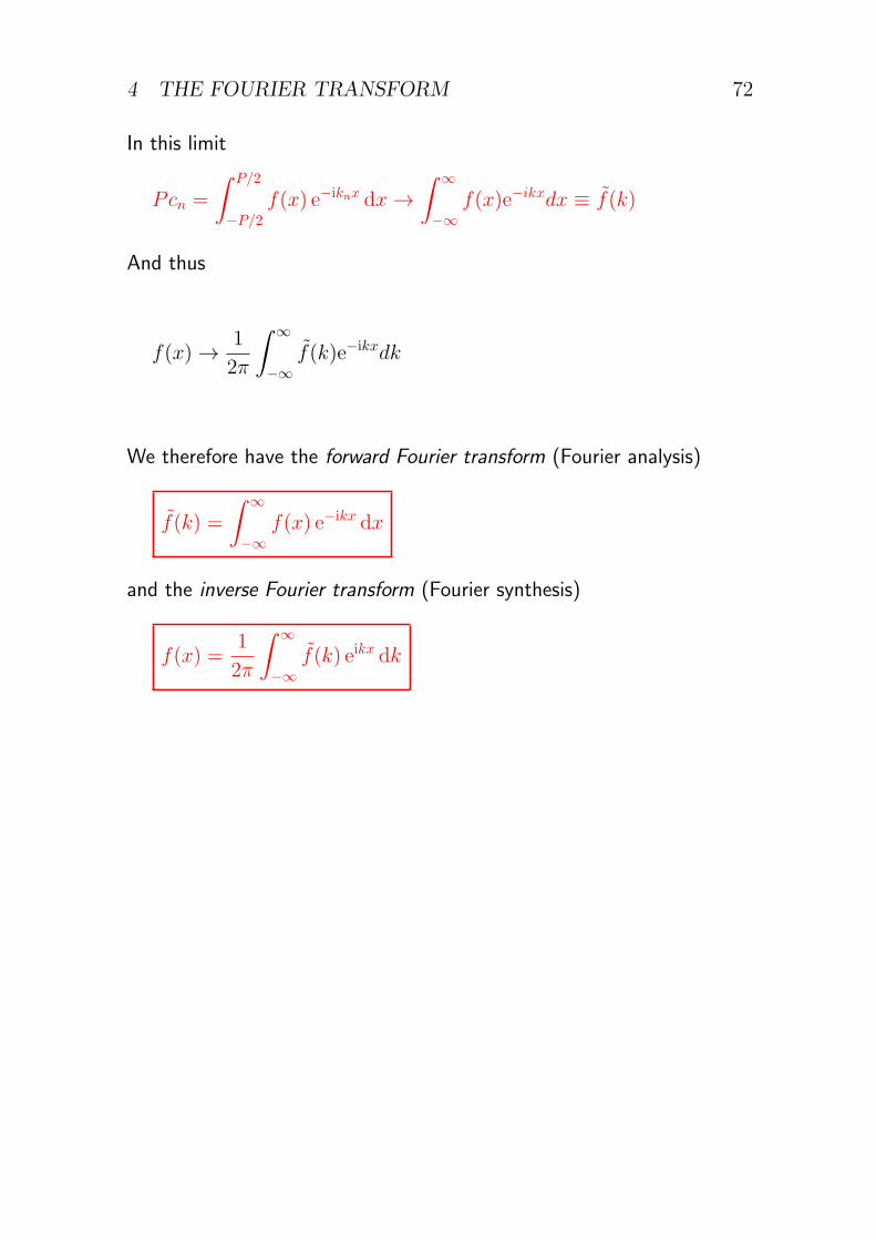
In this limit

Pcn =

∫ P/2

−P/2

f(x) e−iknx dx→∫ ∞

−∞f(x)e−ikxdx ≡ f(k)

And thus

f(x) → 1

2π

∫ ∞

−∞f(k)e−ikxdk

We therefore have the forward Fourier transform (Fourier analysis)

f(k) =

∫ ∞

−∞f(x) e−ikx dx

and the inverse Fourier transform (Fourier synthesis)

f(x) =1

2π

∫ ∞

−∞f(k) eikx dk

4 THE FOURIER TRANSFORM 73

Notes:

• the Fourier transform operation is sometimes denoted by

f(k) = F [f(x)], f(x) = F−1[f(k)]

• the variables are often called t and ω rather than x and k (time ↔angular frequency vs. position ↔ wavenumber)

• it is sometimes useful to consider complex values of k

• for a rigorous proof, certain technical conditions on f(x) are required:

A necessary condition for f(k) to exist for all real values of k (in the sense

of an ordinary function) is that f(x) → 0 as x → ±∞. Otherwise the

Fourier integral does not converge (e.g. for k = 0).

A set of sufficient conditions for f(k) to exist is that f(x) have ‘bounded

variation’, have a finite number of discontinuities and be ‘absolutely inte-

grable’, i.e.∫ ∞

−∞|f(x)| dx <∞.

However, we will see that Fourier transforms can be assigned in a wider

sense to some functions that do not satisfy all of these conditions, e.g.

f(x) = 1.

Warning 2. Several different definitions of the Fourier transform are

in use. They differ in the placement of the 2π factor and in the signs

of the exponents. The definition used here is probably the most con-

ventional.

How to remember this convention:

• the sign of the exponent is different in the forward and inverse trans-

forms

4 THE FOURIER TRANSFORM 74

• the inverse transform means that the function f(x) is synthesized from

a linear combination of basis functions eikx

• the division by 2π always accompanies integration with respect to k

4 THE FOURIER TRANSFORM 75

4.3 Examples

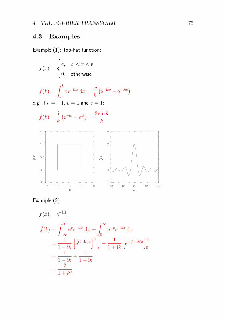
Example (1): top-hat function:

f(x) =

c, a < x < b

0, otherwise

f(k) =

∫ b

a

c e−ikx dx =ic

k

(e−ikb − e−ika

)e.g. if a = −1, b = 1 and c = 1:

f(k) =i

k

(e−ik − eik

)=

2 sin k

k

Example (2):

f(x) = e−|x|

f(k) =

∫ 0

−∞exe−ikx dx+

∫ ∞

0

e−xe−ikx dx

=1

1− ik

[e(1−ik)x

]0−∞

− 1

1 + ik

[e−(1+ik)x

]∞0

=1

1− ik+

1

1 + ik

=2

1 + k2

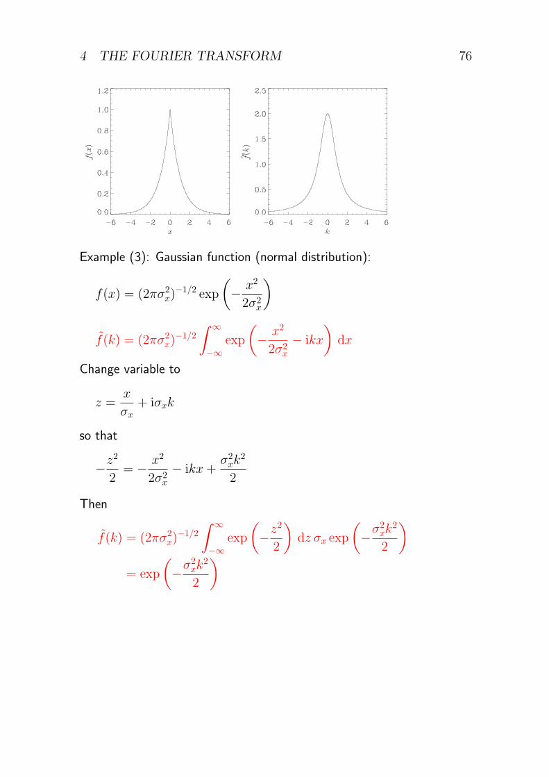
4 THE FOURIER TRANSFORM 76

Example (3): Gaussian function (normal distribution):

f(x) = (2πσ2x)

−1/2 exp

(− x2

2σ2x

)

f(k) = (2πσ2x)

−1/2

∫ ∞

−∞exp

(− x2

2σ2x− ikx

)dx

Change variable to

z =x

σx+ iσxk

so that

−z2

2= − x2

2σ2x− ikx+

σ2xk2

2

Then

f(k) = (2πσ2x)−1/2

∫ ∞

−∞exp

(−z

2

2

)dz σx exp

(−σ

2xk

2

2

)= exp

(−σ

2xk

2

2

)

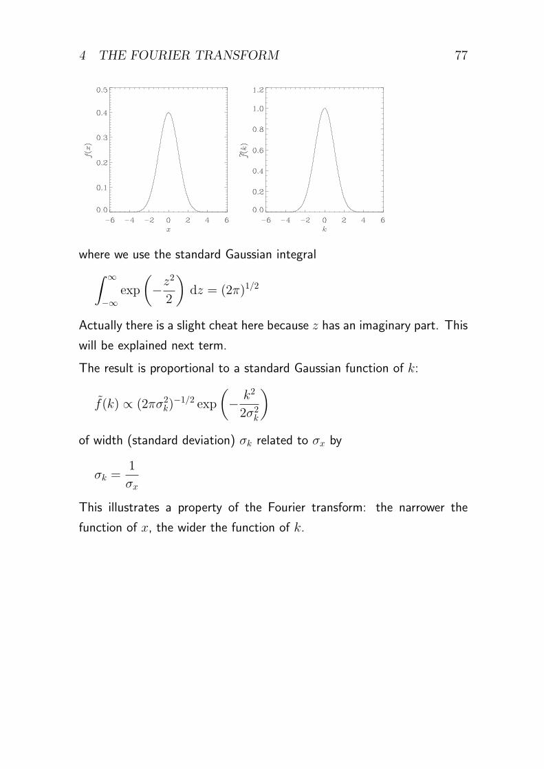
4 THE FOURIER TRANSFORM 77

where we use the standard Gaussian integral∫ ∞

−∞exp

(−z

2

2

)dz = (2π)1/2

Actually there is a slight cheat here because z has an imaginary part. This

will be explained next term.

The result is proportional to a standard Gaussian function of k:

f(k) ∝ (2πσ2k)−1/2 exp

(− k2

2σ2k

)of width (standard deviation) σk related to σx by

σk =1

σx

This illustrates a property of the Fourier transform: the narrower the

function of x, the wider the function of k.

4 THE FOURIER TRANSFORM 78

4.4 Basic properties of the Fourier transform

Linearity:

g(x) = αf(x) ⇔ g(k) = αf(k) (2)

h(x) = f(x) + g(x) ⇔ h(k) = f(k) + g(k) (3)

Rescaling (for real α):

g(x) = f(αx) ⇔ g(k) =1

|α|f

(k

α

)(4)

Shift/exponential (for real α):

g(x) = f(x− α) ⇔ g(k) = e−ikαf(k) (5)

g(x) = eiαxf(x) ⇔ g(k) = f(k − α) (6)

Differentiation/multiplication:

g(x) = f ′(x) ⇔ g(k) = ikf(k) (7)

g(x) = xf(x) ⇔ g(k) = if ′(k) (8)

Duality:

g(x) = f(x) ⇔ g(k) = 2πf(−k) (9)

i.e. transforming twice returns (almost) the same function

Complex conjugation and parity inversion (for real x and k):

g(x) = [f(x)]∗ ⇔ g(k) = [f(−k)]∗ (10)

Symmetry:

f(−x) = ±f(x) ⇔ f(−k) = ±f(k) (11)

4 THE FOURIER TRANSFORM 79

Sample derivations: property (3):

g(x) = f(αx)

g(k) =

∫ ∞

−∞f(αx) e−ikx dx

= sgn (α)

∫ ∞

−∞f(y) e−iky/α dy

α

=1

|α|

∫ ∞

−∞f(y) e−i(k/α)y dy

=1

|α|f

(k

α

)Property (4):

g(x) = f(x− α)

g(k) =

∫ ∞

−∞f(x− α) e−ikx dx

=

∫ ∞

−∞f(y) e−ik(y+α) dy

= e−ikαf(k)

Property (6):

g(x) = f ′(x)

g(k) =

∫ ∞

−∞f ′(x) e−ikx dx

=[f(x) e−ikx

]∞−∞ −

∫ ∞

−∞f(x)(−ik)e−ikx dx

= ikf(k)

The integrated part vanishes because f(x) must tend to zero as x→ ±∞in order to possess a Fourier transform.

4 THE FOURIER TRANSFORM 80

Property (7):

g(x) = xf(x)

g(k) =

∫ ∞

−∞xf(x) e−ikx dx

= i

∫ ∞

−∞f(x)(−ix)e−ikx dx

= id

dk

∫ ∞

−∞f(x) e−ikx dx

= if ′(k)

Property (8):

g(x) = f(x)

g(k) =

∫ ∞

−∞f(x) e−ikx dx

= 2πf(−k)

Property (10): if f(−x) = ±f(x), i.e. f is even or odd, then

f(−k) =∫ ∞

−∞f(x) e+ikx dx

=

∫ ∞

−∞±f(−x) eikx dx

= ±∫ ∞

−∞f(y) e−iky dy

= ±f(k)

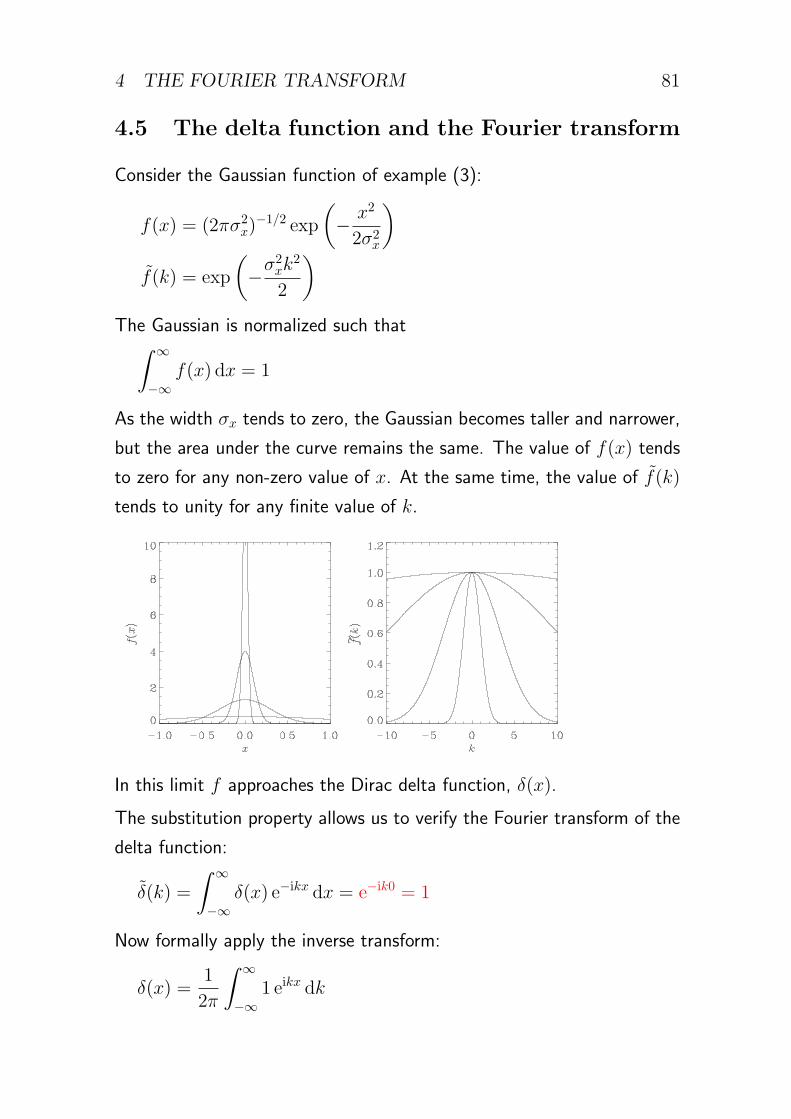
4 THE FOURIER TRANSFORM 81

4.5 The delta function and the Fourier transform

Consider the Gaussian function of example (3):

f(x) = (2πσ2x)

−1/2 exp

(− x2

2σ2x

)f(k) = exp

(−σ

2xk

2

2

)The Gaussian is normalized such that∫ ∞

−∞f(x) dx = 1

As the width σx tends to zero, the Gaussian becomes taller and narrower,

but the area under the curve remains the same. The value of f(x) tends

to zero for any non-zero value of x. At the same time, the value of f(k)

tends to unity for any finite value of k.

In this limit f approaches the Dirac delta function, δ(x).

The substitution property allows us to verify the Fourier transform of the

delta function:

δ(k) =

∫ ∞

−∞δ(x) e−ikx dx = e−ik0 = 1

Now formally apply the inverse transform:

δ(x) =1

2π

∫ ∞

−∞1 eikx dk

4 THE FOURIER TRANSFORM 82

Relabel the variables and rearrange (the exponent can have either sign):∫ ∞

−∞e±ikx dx = 2πδ(k)

Therefore the Fourier transform of a unit constant (1) is 2πδ(k). Note

that a constant function does not satisfy the necessary condition for the

existence of a (regular) Fourier transform. But it does have a Fourier

transform in the space of generalized functions.

4.6 The convolution theorem

4.6.1 Definition of convolution

The convolution of two functions, h = f ∗ g, is defined by

h(x) =

∫ ∞

−∞f(y)g(x− y) dy

Note that the sum of the arguments of f and g is the argument of h.

Convolution is a symmetric operation:

[g ∗ f ](x) =∫ ∞

−∞g(y)f(x− y) dy

=

∫ ∞

−∞f(z)g(x− z) dz

= [f ∗ g](x)

4.6.2 Interpretation and examples

In statistics, a continuous random variable x (e.g. the height of a person

drawn at random from the population) has a probability distribution (or

density) function f(x). The probability of x lying in the range x0 < x <

x0 + δx is f(x0)δx, in the limit of small δx.

4 THE FOURIER TRANSFORM 83

If x and y are independent random variables with distribution functions

f(x) and g(y), then let the distribution function of their sum, z = x+ y,

be h(z). (E.g. let y be the height of a pair of shoes drawn at random.

Then z is the height of a random person while wearing a random pair of

shoes.)

Now, for any given value of x, the probability that z lies in the range

z0 < z < z0 + δz

is just the probability that y lies in the range

z0 − x < y < z0 − x+ δz

which is g(z0 − x)δz. Therefore

h(z0)δz =

∫ ∞

−∞f(x)g(z0 − x)δz dx

which implies

h = f ∗ g

The effect of measuring, observing or processing scientific data can often

be described as a convolution of the data with a certain function.

e.g. when a point source is observed by a telescope, a broadened image

is seen, known as the point spread function of the telescope. When an

extended source is observed, the image that is seen is the convolution of

the source with the point spread function.

In this sense convolution corresponds to a broadening or distortion of the

original data.

A point mass M at position R gives rise to a gravitational potential

Φp(r) = −GM/|r−R|. A continuous mass density ρ(r) can be thought

of as a sum of infinitely many point masses ρ(R) d3R at positions R.

The resulting gravitational potential is

Φ(r) = −G∫

ρ(R)

|r −R|d3R

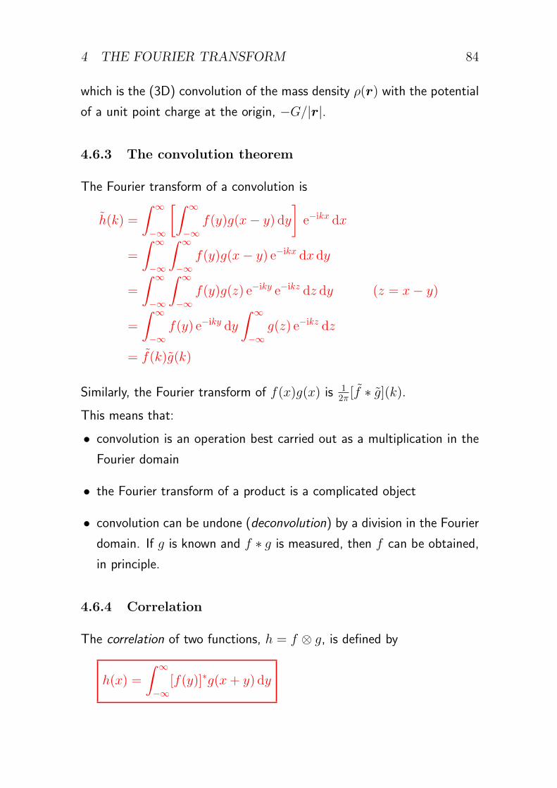
4 THE FOURIER TRANSFORM 84

which is the (3D) convolution of the mass density ρ(r) with the potential

of a unit point charge at the origin, −G/|r|.

4.6.3 The convolution theorem

The Fourier transform of a convolution is

h(k) =

∫ ∞

−∞

[∫ ∞

−∞f(y)g(x− y) dy

]e−ikx dx

=

∫ ∞

−∞

∫ ∞

−∞f(y)g(x− y) e−ikx dx dy

=

∫ ∞

−∞

∫ ∞

−∞f(y)g(z) e−iky e−ikz dz dy (z = x− y)

=

∫ ∞

−∞f(y) e−iky dy

∫ ∞

−∞g(z) e−ikz dz

= f(k)g(k)

Similarly, the Fourier transform of f(x)g(x) is 12π [f ∗ g](k).

This means that:

• convolution is an operation best carried out as a multiplication in the

Fourier domain

• the Fourier transform of a product is a complicated object

• convolution can be undone (deconvolution) by a division in the Fourier

domain. If g is known and f ∗ g is measured, then f can be obtained,

in principle.

4.6.4 Correlation

The correlation of two functions, h = f ⊗ g, is defined by

h(x) =

∫ ∞

−∞[f(y)]∗g(x+ y) dy

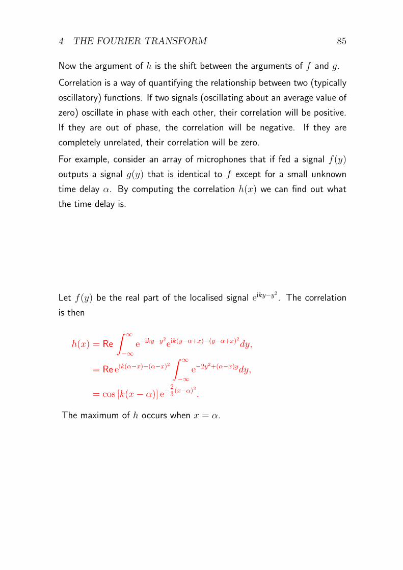
4 THE FOURIER TRANSFORM 85

Now the argument of h is the shift between the arguments of f and g.

Correlation is a way of quantifying the relationship between two (typically

oscillatory) functions. If two signals (oscillating about an average value of

zero) oscillate in phase with each other, their correlation will be positive.

If they are out of phase, the correlation will be negative. If they are

completely unrelated, their correlation will be zero.

For example, consider an array of microphones that if fed a signal f(y)

outputs a signal g(y) that is identical to f except for a small unknown

time delay α. By computing the correlation h(x) we can find out what

the time delay is.

Let f(y) be the real part of the localised signal eiky−y2. The correlation

is then

h(x) = Re

∫ ∞

−∞e−iky−y2eik(y−α+x)−(y−α+x)2dy,

= Re eik(α−x)−(α−x)2∫ ∞

−∞e−2y2+(α−x)ydy,

= cos [k(x− α)] e−23(x−α)2.

The maximum of h occurs when x = α.

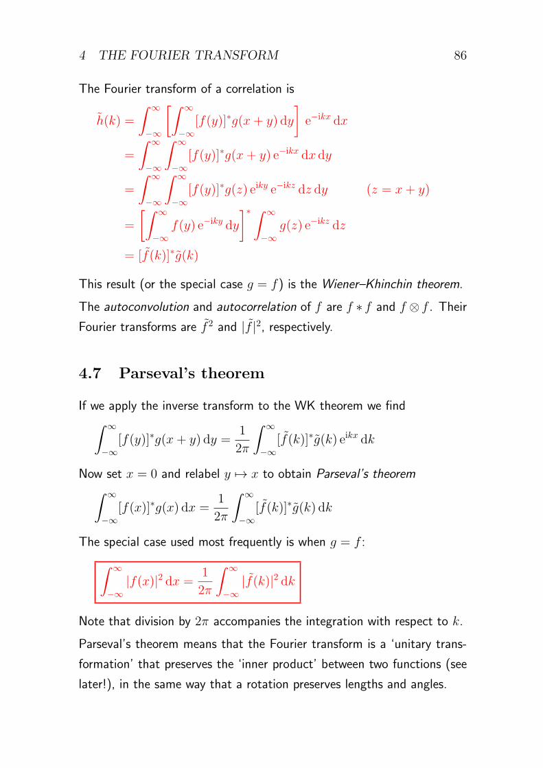
4 THE FOURIER TRANSFORM 86

The Fourier transform of a correlation is

h(k) =

∫ ∞

−∞

[∫ ∞

−∞[f(y)]∗g(x+ y) dy

]e−ikx dx

=

∫ ∞

−∞

∫ ∞

−∞[f(y)]∗g(x+ y) e−ikx dx dy

=

∫ ∞

−∞

∫ ∞

−∞[f(y)]∗g(z) eiky e−ikz dz dy (z = x+ y)

=

[∫ ∞

−∞f(y) e−iky dy

]∗ ∫ ∞

−∞g(z) e−ikz dz

= [f(k)]∗g(k)

This result (or the special case g = f) is the Wiener–Khinchin theorem.

The autoconvolution and autocorrelation of f are f ∗ f and f ⊗ f . Their

Fourier transforms are f 2 and |f |2, respectively.

4.7 Parseval’s theorem

If we apply the inverse transform to the WK theorem we find∫ ∞

−∞[f(y)]∗g(x+ y) dy =

1

2π

∫ ∞

−∞[f(k)]∗g(k) eikx dk

Now set x = 0 and relabel y 7→ x to obtain Parseval’s theorem∫ ∞

−∞[f(x)]∗g(x) dx =

1

2π

∫ ∞

−∞[f(k)]∗g(k) dk

The special case used most frequently is when g = f :∫ ∞

−∞|f(x)|2 dx =

1

2π

∫ ∞

−∞|f(k)|2 dk

Note that division by 2π accompanies the integration with respect to k.

Parseval’s theorem means that the Fourier transform is a ‘unitary trans-

formation’ that preserves the ‘inner product’ between two functions (see

later!), in the same way that a rotation preserves lengths and angles.

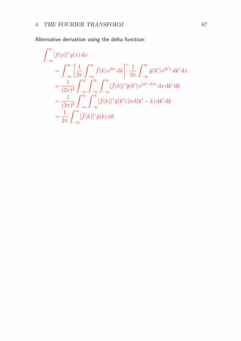
4 THE FOURIER TRANSFORM 87

Alternative derivation using the delta function:∫ ∞

−∞[f(x)]∗g(x) dx

=

∫ ∞

−∞

[1

2π

∫ ∞

−∞f(k) eikx dk

]∗1

2π

∫ ∞

−∞g(k′) eik

′x dk′ dx

=1

(2π)2

∫ ∞

−∞

∫ ∞

−∞

∫ ∞

−∞[f(k)]∗g(k′) ei(k

′−k)x dx dk′ dk

=1

(2π)2

∫ ∞

−∞

∫ ∞

−∞[f(k)]∗g(k′) 2πδ(k′ − k) dk′ dk

=1

2π

∫ ∞

−∞[f(k)]∗g(k) dk

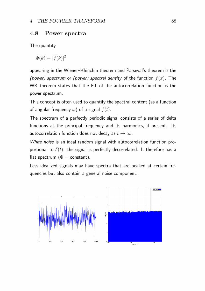
4 THE FOURIER TRANSFORM 88

4.8 Power spectra

The quantity

Φ(k) = |f(k)|2

appearing in the Wiener–Khinchin theorem and Parseval’s theorem is the

(power) spectrum or (power) spectral density of the function f(x). The

WK theorem states that the FT of the autocorrelation function is the

power spectrum.

This concept is often used to quantify the spectral content (as a function

of angular frequency ω) of a signal f(t).

The spectrum of a perfectly periodic signal consists of a series of delta

functions at the principal frequency and its harmonics, if present. Its

autocorrelation function does not decay as t→ ∞.

White noise is an ideal random signal with autocorrelation function pro-

portional to δ(t): the signal is perfectly decorrelated. It therefore has a

flat spectrum (Φ = constant).

Less idealized signals may have spectra that are peaked at certain fre-

quencies but also contain a general noise component.

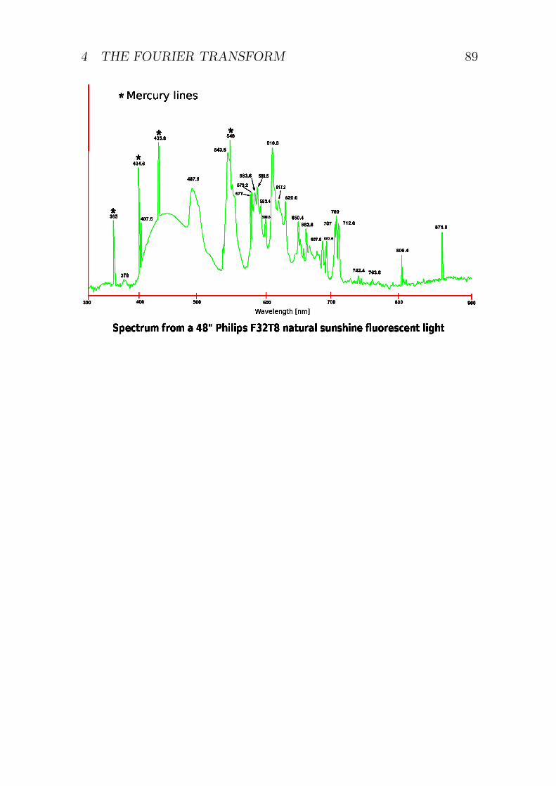
4 THE FOURIER TRANSFORM 89

5 MATRICES AND LINEAR ALGEBRA 90

5 Matrices and linear algebra

5.1 Motivation

Many scientific quantities are vectors. A linear relationship between two

vectors is described by a matrix. This could be either

• a physical relationship, e.g. that between the angular velocity and an-

gular momentum vectors of a rotating body

• a relationship between the components of (physically) the same vector

in different coordinate systems

Linear algebra deals with the addition and multiplication of scalars, vectors

and matrices.

Eigenvalues and eigenvectors are the characteristic numbers and direc-

tions associated with matrices, which allow them to be expressed in the

simplest form. The matrices that occur in scientific applications usually

have special symmetries that impose conditions on their eigenvalues and

eigenvectors.

Vectors do not necessarily live in physical space. In some applications

(notably quantum mechanics) we have to deal with complex spaces of

various dimensions.

5.2 Vector spaces

5.2.1 Abstract definition of scalars and vectors

We are used to thinking of scalars as numbers, and vectors as directed

line segments. For many purposes it is useful to define scalars and vectors

in a more general (and abstract) way.

5 MATRICES AND LINEAR ALGEBRA 91

Scalars are the elements of a number field, of which the most important

examples are:

• R, the set of real numbers

• C, the set of complex numbers

A number field F :

• is a set of elements on which the operations of addition and multiplica-

tion are defined and satisfy the usual laws of arithmetic (commutative,

associative and distributive)

• is closed under addition and multiplication

• includes identity elements (the numbers 0 and 1) for addition and

multiplication

• includes inverses (negatives and reciprocals) for addition and multipli-

cation for every element, except that 0 has no reciprocal

Vectors are the elements of a vector space (or linear space) defined over

a number field F .

A vector space V :

• is a set of elements on which the operations of vector addition and

scalar multiplication are defined and satisfy certain axioms

• is closed under these operations

• includes an identity element (the vector 0) for vector addition

We will write vectors in bold italic face (or underlined in handwriting).

Scalar multiplication means multiplying a vector x by a scalar α to obtain

the vector αx. Note that 0x = 0 and 1x = x.

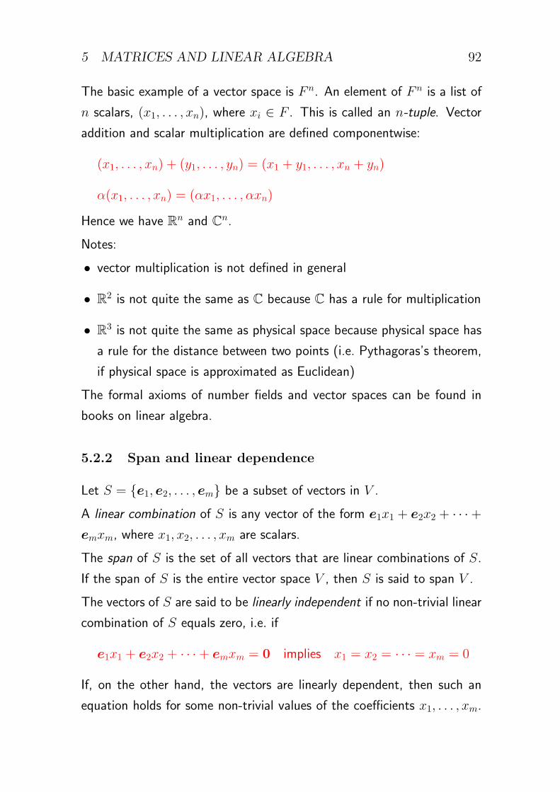
5 MATRICES AND LINEAR ALGEBRA 92

The basic example of a vector space is F n. An element of F n is a list of

n scalars, (x1, . . . , xn), where xi ∈ F . This is called an n-tuple. Vector

addition and scalar multiplication are defined componentwise:

(x1, . . . , xn) + (y1, . . . , yn) = (x1 + y1, . . . , xn + yn)

α(x1, . . . , xn) = (αx1, . . . , αxn)

Hence we have Rn and Cn.

Notes:

• vector multiplication is not defined in general

• R2 is not quite the same as C because C has a rule for multiplication

• R3 is not quite the same as physical space because physical space has

a rule for the distance between two points (i.e. Pythagoras’s theorem,

if physical space is approximated as Euclidean)

The formal axioms of number fields and vector spaces can be found in

books on linear algebra.

5.2.2 Span and linear dependence

Let S = {e1, e2, . . . , em} be a subset of vectors in V .

A linear combination of S is any vector of the form e1x1 + e2x2 + · · ·+emxm, where x1, x2, . . . , xm are scalars.

The span of S is the set of all vectors that are linear combinations of S.

If the span of S is the entire vector space V , then S is said to span V .

The vectors of S are said to be linearly independent if no non-trivial linear

combination of S equals zero, i.e. if

e1x1 + e2x2 + · · ·+ emxm = 0 implies x1 = x2 = · · · = xm = 0

If, on the other hand, the vectors are linearly dependent, then such an

equation holds for some non-trivial values of the coefficients x1, . . . , xm.

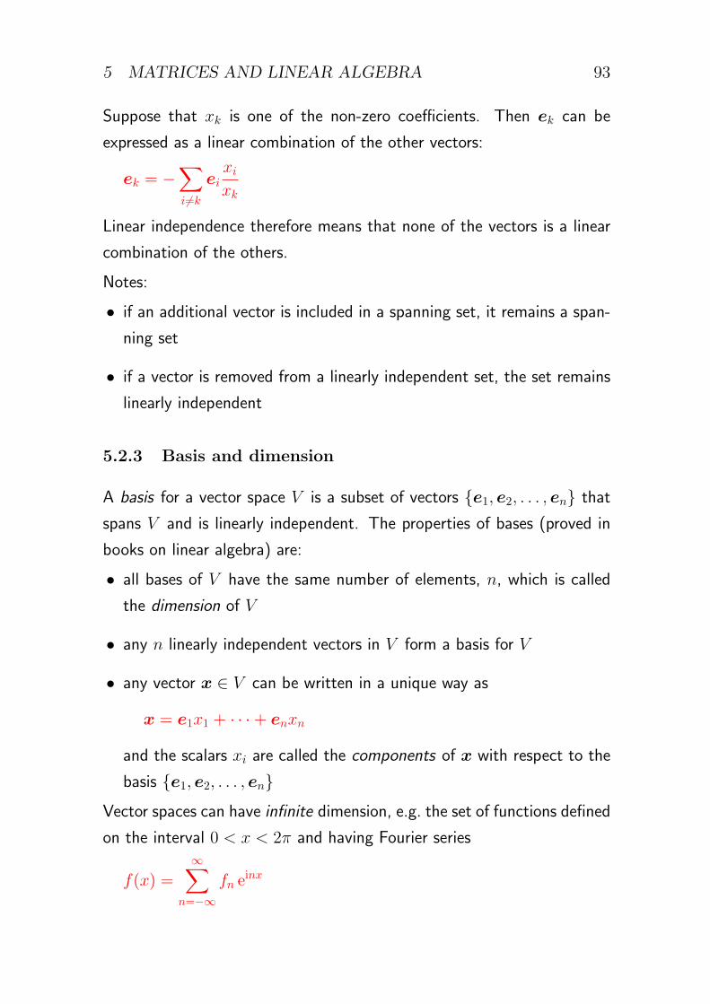
5 MATRICES AND LINEAR ALGEBRA 93

Suppose that xk is one of the non-zero coefficients. Then ek can be

expressed as a linear combination of the other vectors:

ek = −∑i=k

eixixk

Linear independence therefore means that none of the vectors is a linear

combination of the others.

Notes:

• if an additional vector is included in a spanning set, it remains a span-

ning set

• if a vector is removed from a linearly independent set, the set remains

linearly independent

5.2.3 Basis and dimension

A basis for a vector space V is a subset of vectors {e1, e2, . . . , en} that

spans V and is linearly independent. The properties of bases (proved in

books on linear algebra) are:

• all bases of V have the same number of elements, n, which is called

the dimension of V

• any n linearly independent vectors in V form a basis for V

• any vector x ∈ V can be written in a unique way as

x = e1x1 + · · ·+ enxn

and the scalars xi are called the components of x with respect to the

basis {e1, e2, . . . , en}

Vector spaces can have infinite dimension, e.g. the set of functions defined

on the interval 0 < x < 2π and having Fourier series

f(x) =∞∑

n=−∞fn e

inx

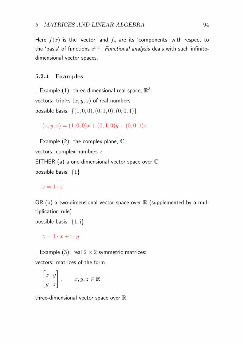
5 MATRICES AND LINEAR ALGEBRA 94

Here f(x) is the ‘vector’ and fn are its ‘components’ with respect to

the ‘basis’ of functions einx. Functional analysis deals with such infinite-

dimensional vector spaces.

5.2.4 Examples

▷ Example (1): three-dimensional real space, R3:

vectors: triples (x, y, z) of real numbers

possible basis: {(1, 0, 0), (0, 1, 0), (0, 0, 1)}

(x, y, z) = (1, 0, 0)x+ (0, 1, 0)y + (0, 0, 1)z

▷ Example (2): the complex plane, C:

vectors: complex numbers z

EITHER (a) a one-dimensional vector space over C

possible basis: {1}

z = 1 · z

OR (b) a two-dimensional vector space over R (supplemented by a mul-

tiplication rule)

possible basis: {1, i}

z = 1 · x+ i · y

▷ Example (3): real 2× 2 symmetric matrices:

vectors: matrices of the form[x y

y z

], x, y, z ∈ R

three-dimensional vector space over R

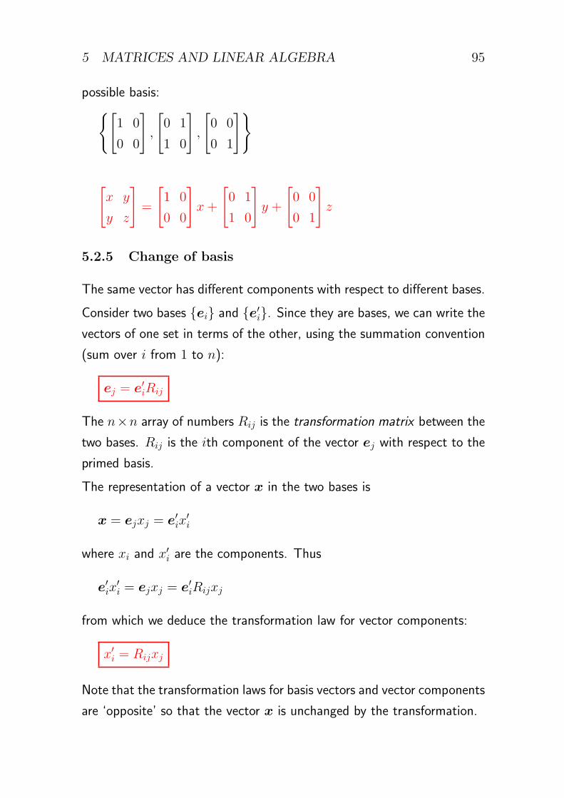
5 MATRICES AND LINEAR ALGEBRA 95

possible basis:{[1 0

0 0

],

[0 1

1 0

],

[0 0

0 1

]}

[x y

y z

]=

[1 0

0 0

]x+

[0 1

1 0

]y +

[0 0

0 1

]z

5.2.5 Change of basis

The same vector has different components with respect to different bases.

Consider two bases {ei} and {e′i}. Since they are bases, we can write the

vectors of one set in terms of the other, using the summation convention

(sum over i from 1 to n):

ej = e′iRij

The n×n array of numbers Rij is the transformation matrix between the

two bases. Rij is the ith component of the vector ej with respect to the

primed basis.

The representation of a vector x in the two bases is

x = ejxj = e′ix′i

where xi and x′i are the components. Thus

e′ix′i = ejxj = e′iRijxj

from which we deduce the transformation law for vector components:

x′i = Rijxj

Note that the transformation laws for basis vectors and vector components

are ‘opposite’ so that the vector x is unchanged by the transformation.

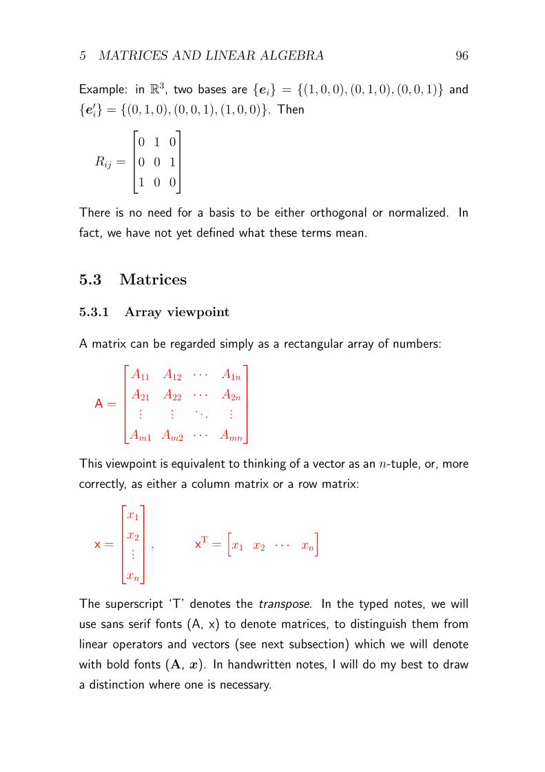
5 MATRICES AND LINEAR ALGEBRA 96

Example: in R3, two bases are {ei} = {(1, 0, 0), (0, 1, 0), (0, 0, 1)} and

{e′i} = {(0, 1, 0), (0, 0, 1), (1, 0, 0)}. Then

Rij =

0 1 0

0 0 1

1 0 0

There is no need for a basis to be either orthogonal or normalized. In

fact, we have not yet defined what these terms mean.

5.3 Matrices

5.3.1 Array viewpoint

A matrix can be regarded simply as a rectangular array of numbers:

A =

A11 A12 · · · A1n

A21 A22 · · · A2n...

... . . . ...

Am1 Am2 · · · Amn

This viewpoint is equivalent to thinking of a vector as an n-tuple, or, more

correctly, as either a column matrix or a row matrix:

x =

x1

x2...

xn

, xT =[x1 x2 · · · xn

]

The superscript ‘T’ denotes the transpose. In the typed notes, we will

use sans serif fonts (A, x) to denote matrices, to distinguish them from

linear operators and vectors (see next subsection) which we will denote

with bold fonts (A, x). In handwritten notes, I will do my best to draw

a distinction where one is necessary.

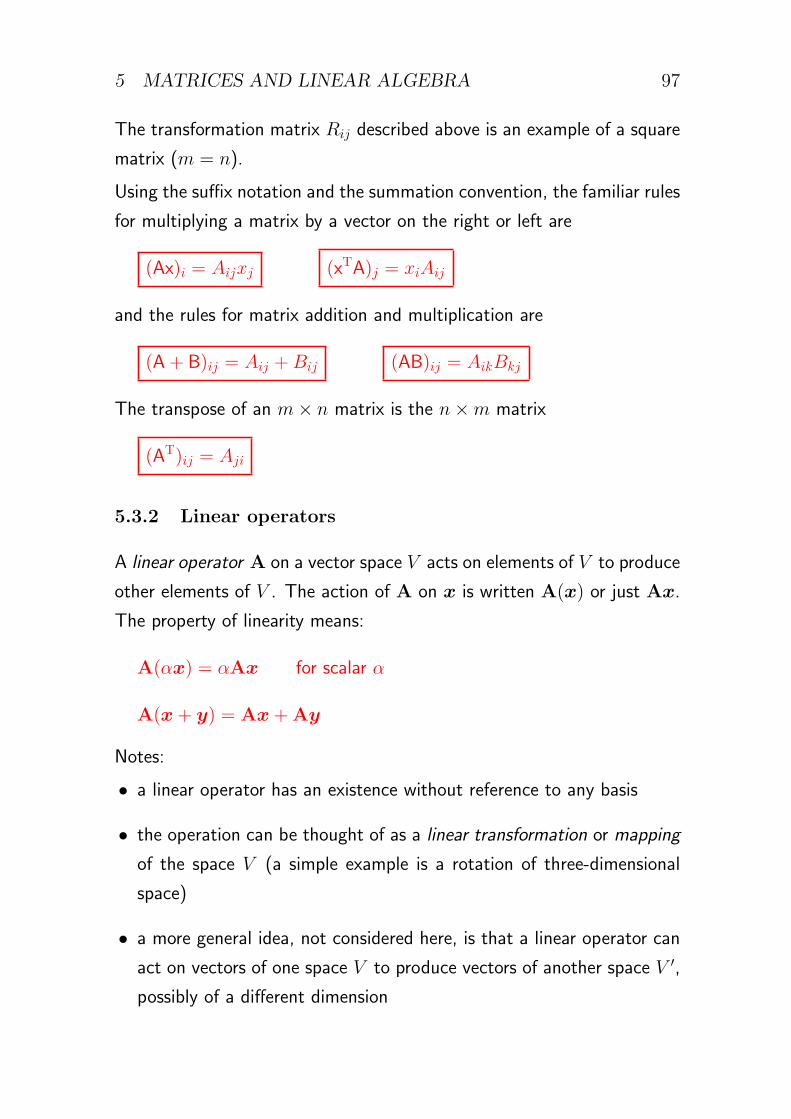
5 MATRICES AND LINEAR ALGEBRA 97

The transformation matrix Rij described above is an example of a square

matrix (m = n).

Using the suffix notation and the summation convention, the familiar rules

for multiplying a matrix by a vector on the right or left are

(Ax)i = Aijxj (xTA)j = xiAij

and the rules for matrix addition and multiplication are

(A+ B)ij = Aij +Bij (AB)ij = AikBkj

The transpose of an m× n matrix is the n×m matrix

(AT)ij = Aji

5.3.2 Linear operators

A linear operator A on a vector space V acts on elements of V to produce

other elements of V . The action of A on x is written A(x) or just Ax.

The property of linearity means:

A(αx) = αAx for scalar α

A(x+ y) = Ax+Ay

Notes:

• a linear operator has an existence without reference to any basis

• the operation can be thought of as a linear transformation or mapping

of the space V (a simple example is a rotation of three-dimensional

space)

• a more general idea, not considered here, is that a linear operator can

act on vectors of one space V to produce vectors of another space V ′,

possibly of a different dimension

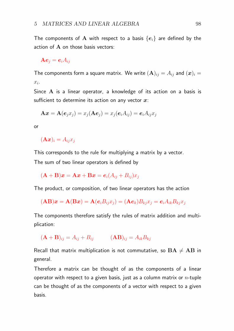
5 MATRICES AND LINEAR ALGEBRA 98

The components of A with respect to a basis {ei} are defined by the

action of A on those basis vectors:

Aej = eiAij

The components form a square matrix. We write (A)ij = Aij and (x)i =

xi.

Since A is a linear operator, a knowledge of its action on a basis is

sufficient to determine its action on any vector x:

Ax = A(ejxj) = xj(Aej) = xj(eiAij) = eiAijxj

or

(Ax)i = Aijxj

This corresponds to the rule for multiplying a matrix by a vector.

The sum of two linear operators is defined by

(A+B)x = Ax+Bx = ei(Aij +Bij)xj

The product, or composition, of two linear operators has the action

(AB)x = A(Bx) = A(eiBijxj) = (Aek)Bkjxj = eiAikBkjxj

The components therefore satisfy the rules of matrix addition and multi-

plication:

(A+B)ij = Aij +Bij (AB)ij = AikBkj

Recall that matrix multiplication is not commutative, so BA = AB in

general.

Therefore a matrix can be thought of as the components of a linear

operator with respect to a given basis, just as a column matrix or n-tuple

can be thought of as the components of a vector with respect to a given

basis.

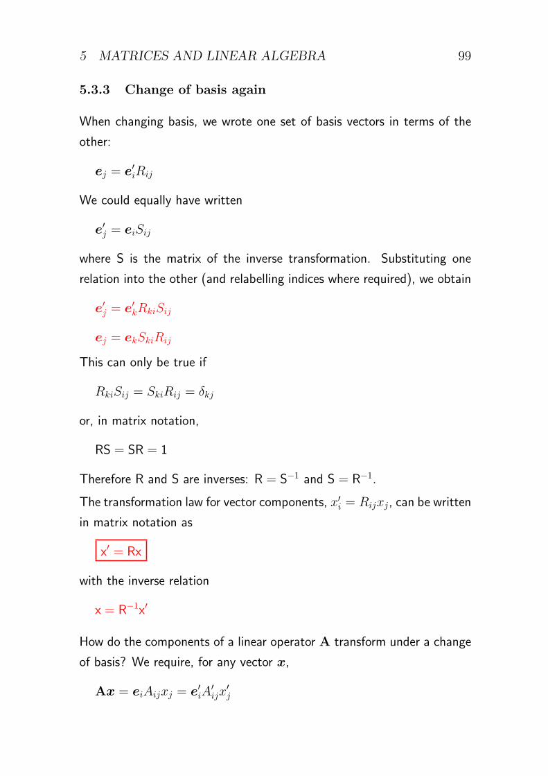
5 MATRICES AND LINEAR ALGEBRA 99

5.3.3 Change of basis again

When changing basis, we wrote one set of basis vectors in terms of the

other:

ej = e′iRij

We could equally have written

e′j = eiSij

where S is the matrix of the inverse transformation. Substituting one

relation into the other (and relabelling indices where required), we obtain

e′j = e′kRkiSij

ej = ekSkiRij

This can only be true if

RkiSij = SkiRij = δkj

or, in matrix notation,

RS = SR = 1

Therefore R and S are inverses: R = S−1 and S = R−1.

The transformation law for vector components, x′i = Rijxj, can be written

in matrix notation as

x′ = Rx

with the inverse relation

x = R−1x′

How do the components of a linear operator A transform under a change

of basis? We require, for any vector x,

Ax = eiAijxj = e′iA′ijx

′j

5 MATRICES AND LINEAR ALGEBRA 100

Using ej = e′iRij and relabelling indices, we find

e′kRkiAijxj = e′kA′kjx

′j

RkiAijxj = A′kjx

′j

RA(R−1x′) = A′x′

Since this is true for any x′, we have

A′ = RAR−1

These transformation laws are consistent, e.g.

A′x′ = RAR−1Rx = RAx = (Ax)′

A′B′ = RAR−1RBR−1 = RABR−1 = (AB)′

5.4 Inner product (scalar product)

This is used to give a meaning to lengths and angles in a vector space.

5.4.1 Definition

An inner product (or scalar product) is a scalar function ⟨x|y⟩ of two

vectors x and y. Other common notations are (x,y), ⟨x,y⟩ and x · y.An inner product must:

• be linear in the second argument:

⟨x|αy⟩ = α⟨x|y⟩ for scalar α

⟨x|y + z⟩ = ⟨x|y⟩+ ⟨x|z⟩

• have Hermitian symmetry :

⟨y|x⟩ = ⟨x|y⟩∗

5 MATRICES AND LINEAR ALGEBRA 101

• be positive definite:

⟨x|x⟩ ⩾ 0 with equality if and only if x = 0

Notes:

• an inner product has an existence without reference to any basis

• the star is needed to ensure that ⟨x|x⟩ is real

• the star is not needed in a real vector space

• it follows that the inner product is antilinear in the first argument:

⟨αx|y⟩ = α∗⟨x|y⟩ for scalar α

⟨x+ y|z⟩ = ⟨x|z⟩+ ⟨y|z⟩

The standard (Euclidean) inner product on Rn is the ‘dot product’

⟨x|y⟩ = x · y = xiyi

which is generalized to Cn as

⟨x|y⟩ = x∗iyi

The star is needed for Hermitian symmetry. We will see later that any

other inner product on Rn or Cn can be reduced to this one by a suitable

choice of basis.

⟨x|x⟩1/2 is the ‘length’ or ‘norm’ of the vector x, written |x| or ∥x∥. Inone dimension this agrees with the meaning of ‘absolute value’ if we are

using the dot product.

5.4.2 The Cauchy–Schwarz inequality

|⟨x|y⟩|2 ⩽ ⟨x|x⟩⟨y|y⟩

5 MATRICES AND LINEAR ALGEBRA 102

or equivalently

|⟨x|y⟩| ⩽ |x||y|

with equality if and only if x = αy (i.e. the vectors are parallel or an-

tiparallel).

Proof: We assume that x = 0 and y = 0, otherwise the inequality is

trivial. We consider the non-negative quantity

⟨x− αy|x− αy⟩ = ⟨x− αy|x⟩ − α⟨x− αy|y⟩

= ⟨x|x⟩ − α∗⟨y|x⟩ − α⟨x|y⟩+ αα∗⟨y|y⟩

= ⟨x|x⟩+ αα∗⟨y|y⟩ − α⟨x|y⟩ − α∗⟨x|y⟩∗

= |x|2 + |α|2|y|2 − 2Re (α⟨x|y⟩)

This result holds for any scalar α. First choose the phase of α such that

α⟨x|y⟩ is real and non-negative and therefore equal to |α||⟨x|y⟩|. Then

|x|2 + |α|2|y|2 − 2|α||⟨x|y⟩| ⩾ 0

(|x| − |α||y|)2 + 2|α||x||y| − 2|α||⟨x|y⟩| ⩾ 0

Now choose the modulus of α such that |α| = |x|/|y|, which is finite

and non-zero. Then divide the inequality by 2|α| to obtain

|x||y| − |⟨x|y⟩| ⩾ 0

as required.

In a real vector space, the Cauchy–Schwarz inequality allows us to define

the angle θ between two vectors through

⟨x|y⟩ = |x||y| cos θ

If ⟨x|y⟩=0 (in any vector space) the vectors are said to be orthogonal.

5 MATRICES AND LINEAR ALGEBRA 103

5.4.3 Inner product and bases

The inner product is bilinear : it is antilinear in the first argument and

linear in the second argument.

Warning 3. This is the usual convention in physics and applied math-

ematics. In pure mathematics it is usually the other way around.

A knowledge of the inner product of the basis vectors is therefore sufficient

to determine the inner product of any two vectors x and y. Let

⟨ei|ej⟩ = Gij

Then

⟨x|y⟩ = ⟨eixi|ejyj⟩ = x∗iyj⟨ei|ej⟩ = Gijx∗iyj

The n × n array of numbers Gij are the metric coefficients of the basis

{ei}. The Hermitian symmetry of the inner product implies that

⟨y|x⟩ = Gijy∗i xj

is equal to

(⟨x|y⟩)∗ = G∗ijxiy

∗j = G∗

jiy∗i xj

(in the last step we exchanged the summation indices i ↔ j) for all

vectors x and y, and therefore

Gji = G∗ij

We say that the matrix G is Hermitian.

An orthonormal basis is one for which

⟨ei|ej⟩ = δij

5 MATRICES AND LINEAR ALGEBRA 104

in which case the inner product is the standard one

⟨x|y⟩ = x∗iyi

We will see later that it is possible to transform any basis into an or-

thonormal one.

5.5 Hermitian conjugate

5.5.1 Definition and simple properties

We define the Hermitian conjugate of a matrix to be the complex conju-

gate of its transpose:

A† = (AT)∗ (A†)ij = A∗ji

This applies to general rectangular matrices, e.g.

[A11 A12 A13

A21 A22 A23

]†

=

A∗

11 A∗21

A∗12 A∗

22

A∗13 A∗

23

The Hermitian conjugate of a column matrix is

x† =

x1

x2...

xn

†

=[x∗1 x∗2 · · · x∗n

]

Note that

(A†)† = A

The Hermitian conjugate of a product of matrices is

(AB)† = B†A†

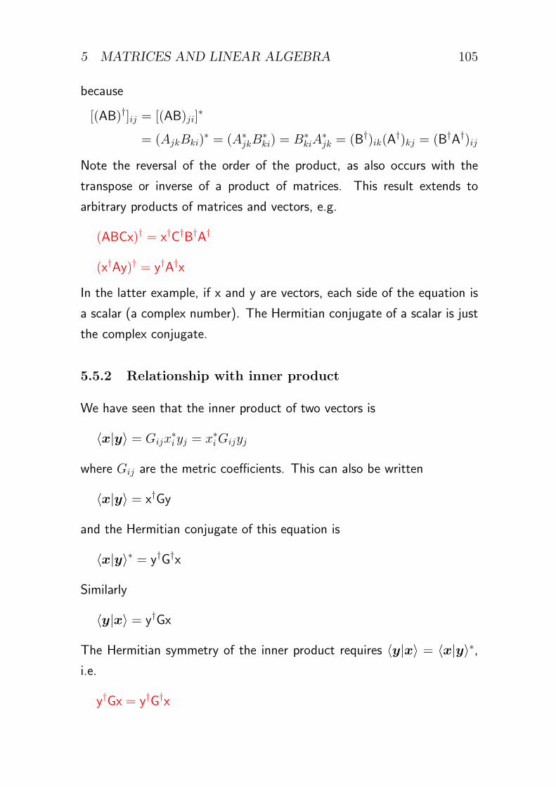
5 MATRICES AND LINEAR ALGEBRA 105

because

[(AB)†]ij = [(AB)ji]∗

= (AjkBki)∗ = (A∗

jkB∗ki) = B∗

kiA∗jk = (B†)ik(A

†)kj = (B†A†)ij

Note the reversal of the order of the product, as also occurs with the

transpose or inverse of a product of matrices. This result extends to

arbitrary products of matrices and vectors, e.g.

(ABCx)† = x†C†B†A†

(x†Ay)† = y†A†x

In the latter example, if x and y are vectors, each side of the equation is

a scalar (a complex number). The Hermitian conjugate of a scalar is just

the complex conjugate.

5.5.2 Relationship with inner product

We have seen that the inner product of two vectors is

⟨x|y⟩ = Gijx∗iyj = x∗iGijyj

where Gij are the metric coefficients. This can also be written

⟨x|y⟩ = x†Gy

and the Hermitian conjugate of this equation is

⟨x|y⟩∗ = y†G†x

Similarly

⟨y|x⟩ = y†Gx

The Hermitian symmetry of the inner product requires ⟨y|x⟩ = ⟨x|y⟩∗,i.e.

y†Gx = y†G†x

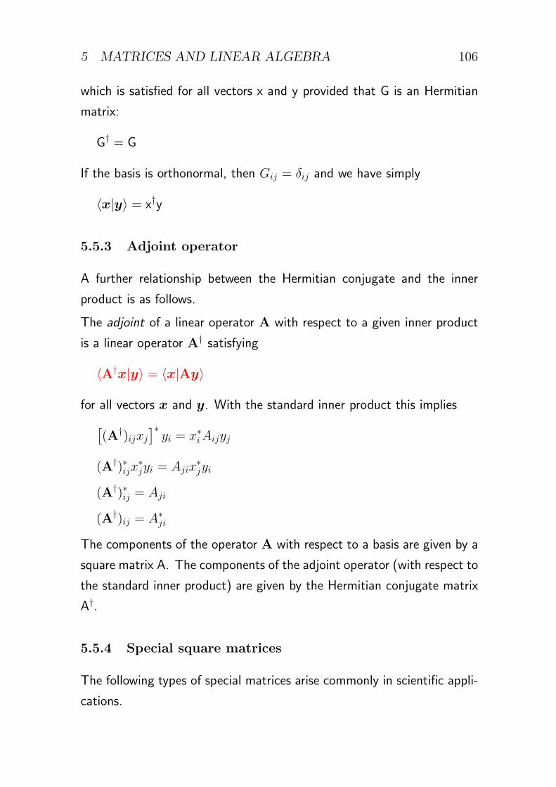
5 MATRICES AND LINEAR ALGEBRA 106

which is satisfied for all vectors x and y provided that G is an Hermitian

matrix:

G† = G

If the basis is orthonormal, then Gij = δij and we have simply

⟨x|y⟩ = x†y

5.5.3 Adjoint operator

A further relationship between the Hermitian conjugate and the inner

product is as follows.

The adjoint of a linear operator A with respect to a given inner product

is a linear operator A† satisfying

⟨A†x|y⟩ = ⟨x|Ay⟩

for all vectors x and y. With the standard inner product this implies[(A†)ijxj

]∗yi = x∗iAijyj

(A†)∗ijx∗jyi = Ajix

∗jyi

(A†)∗ij = Aji

(A†)ij = A∗ji

The components of the operator A with respect to a basis are given by a

square matrix A. The components of the adjoint operator (with respect to

the standard inner product) are given by the Hermitian conjugate matrix

A†.

5.5.4 Special square matrices

The following types of special matrices arise commonly in scientific appli-

cations.

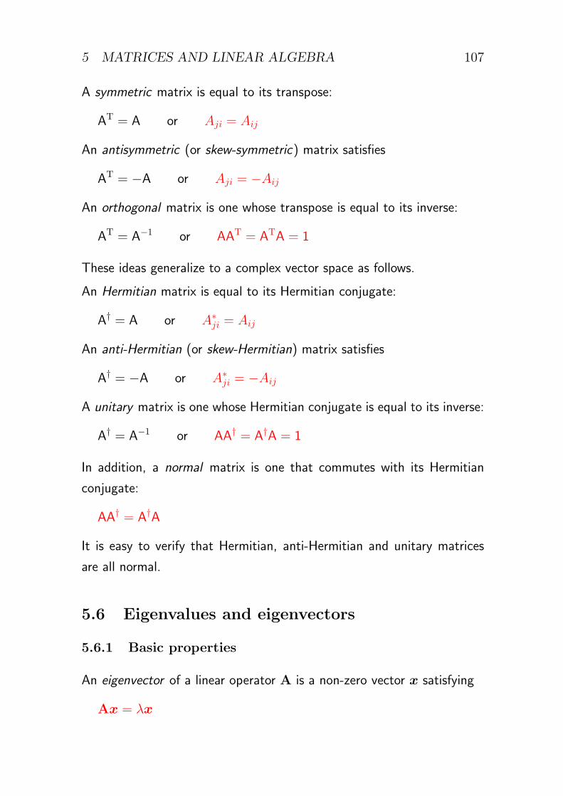
5 MATRICES AND LINEAR ALGEBRA 107

A symmetric matrix is equal to its transpose:

AT = A or Aji = Aij

An antisymmetric (or skew-symmetric) matrix satisfies

AT = −A or Aji = −Aij

An orthogonal matrix is one whose transpose is equal to its inverse:

AT = A−1 or AAT = ATA = 1

These ideas generalize to a complex vector space as follows.

An Hermitian matrix is equal to its Hermitian conjugate:

A† = A or A∗ji = Aij

An anti-Hermitian (or skew-Hermitian) matrix satisfies

A† = −A or A∗ji = −Aij

A unitary matrix is one whose Hermitian conjugate is equal to its inverse:

A† = A−1 or AA† = A†A = 1

In addition, a normal matrix is one that commutes with its Hermitian

conjugate:

AA† = A†A

It is easy to verify that Hermitian, anti-Hermitian and unitary matrices

are all normal.

5.6 Eigenvalues and eigenvectors

5.6.1 Basic properties

An eigenvector of a linear operator A is a non-zero vector x satisfying

Ax = λx

5 MATRICES AND LINEAR ALGEBRA 108

for some scalar λ, the corresponding eigenvalue.

The equivalent statement in a matrix representation is

Ax = λx or (A− λ1)x = 0

where A is an n× n square matrix.

This equation states that a non-trivial linear combination of the columns

of the matrix (A−λ1) is equal to zero, i.e. that the columns of the matrix

are linearly dependent. This is equivalent to the statement

det(A− λ1) = 0

which is the characteristic equation of the matrix A.

To compute the eigenvalues and eigenvectors, we first solve the charac-

teristic equation. This is a polynomial equation of degree n in λ and

therefore has n roots, although not necessarily distinct. These are the

eigenvalues of A, and are complex in general. The corresponding eigen-

vectors are obtained by solving the simultaneous equations found in the

rows of Ax = λx.

If the n roots are distinct, then there are n linearly independent eigenvec-

tors, each of which is determined uniquely up to an arbitrary multiplicative

constant.

If the roots are not all distinct, the repeated eigenvalues are said to be

degenerate. If an eigenvalue λ occurs m times, there may be any number

between 1 and m of linearly independent eigenvectors corresponding to

it. Any linear combination of these is also an eigenvector and the space

spanned by such vectors is called an eigenspace.

Example (1):[0 0

0 0

]

characteristic equation

∣∣∣∣∣0− λ 0

0 0− λ

∣∣∣∣∣ = λ2 = 0

5 MATRICES AND LINEAR ALGEBRA 109

eigenvalues 0, 0

eigenvectors:

[0− λ 0

0 0− λ

][x

y

]=

[0

0

]⇒

[0

0

]=

[0

0

]

two linearly independent eigenvectors, e.g.

[1

0

],

[0

1

]two-dimensional eigenspace corresponding to eigenvalue 0

Example (2):[0 1

0 0

]

characteristic equation

∣∣∣∣∣0− λ 1

0 0− λ

∣∣∣∣∣ = λ2 = 0

eigenvalues 0, 0

eigenvectors:

[0− λ 1

0 0− λ

][x

y

]=

[0

0

]⇒

[y

0

]=

[0

0

]

only one linearly independent eigenvector

[1

0

]one-dimensional eigenspace corresponding to eigenvalue 0

5.6.2 Eigenvalues and eigenvectors of Hermitian matrices

The matrices most often encountered in physical applications are real

symmetric or, more generally, Hermitian matrices satisfying A† = A. In

quantum mechanics, Hermitian matrices (or operators) represent observ-

able quantities.

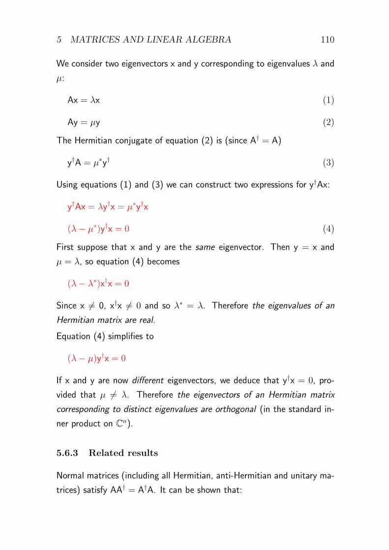
5 MATRICES AND LINEAR ALGEBRA 110

We consider two eigenvectors x and y corresponding to eigenvalues λ and

µ:

Ax = λx (1)

Ay = µy (2)

The Hermitian conjugate of equation (2) is (since A† = A)

y†A = µ∗y† (3)

Using equations (1) and (3) we can construct two expressions for y†Ax:

y†Ax = λy†x = µ∗y†x

(λ− µ∗)y†x = 0 (4)

First suppose that x and y are the same eigenvector. Then y = x and

µ = λ, so equation (4) becomes

(λ− λ∗)x†x = 0

Since x = 0, x†x = 0 and so λ∗ = λ. Therefore the eigenvalues of an

Hermitian matrix are real.

Equation (4) simplifies to

(λ− µ)y†x = 0

If x and y are now different eigenvectors, we deduce that y†x = 0, pro-

vided that µ = λ. Therefore the eigenvectors of an Hermitian matrix

corresponding to distinct eigenvalues are orthogonal (in the standard in-

ner product on Cn).

5.6.3 Related results

Normal matrices (including all Hermitian, anti-Hermitian and unitary ma-

trices) satisfy AA† = A†A. It can be shown that:

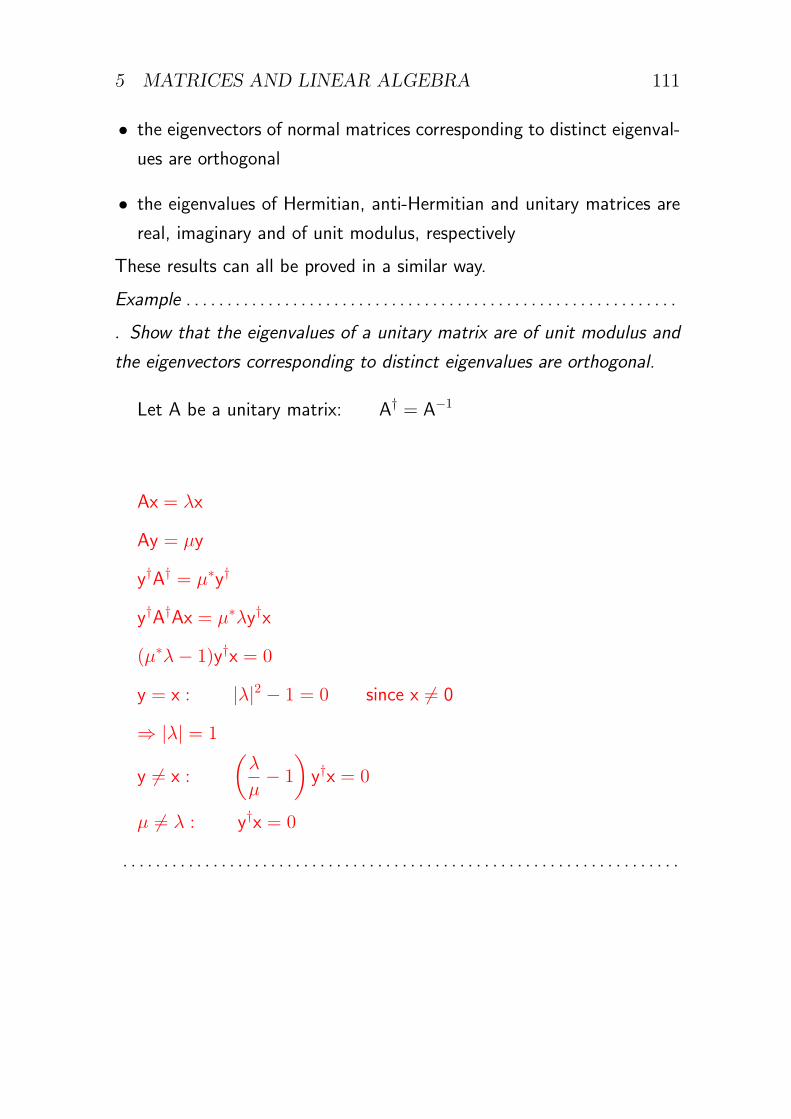
5 MATRICES AND LINEAR ALGEBRA 111

• the eigenvectors of normal matrices corresponding to distinct eigenval-

ues are orthogonal

• the eigenvalues of Hermitian, anti-Hermitian and unitary matrices are

real, imaginary and of unit modulus, respectively

These results can all be proved in a similar way.

Example . . . . . . . . . . . . . . . . . . . . . . . . . . . . . . . . . . . . . . . . . . . . . . . . . . . . . . . . . . . .

▷ Show that the eigenvalues of a unitary matrix are of unit modulus and

the eigenvectors corresponding to distinct eigenvalues are orthogonal.

Let A be a unitary matrix: A† = A−1

Ax = λx

Ay = µy

y†A† = µ∗y†

y†A†Ax = µ∗λy†x

(µ∗λ− 1)y†x = 0

y = x : |λ|2 − 1 = 0 since x = 0

⇒ |λ| = 1

y = x :

(λ

µ− 1

)y†x = 0

µ = λ : y†x = 0

. . . . . . . . . . . . . . . . . . . . . . . . . . . . . . . . . . . . . . . . . . . . . . . . . . . . . . . . . . . . . . . . . . . .

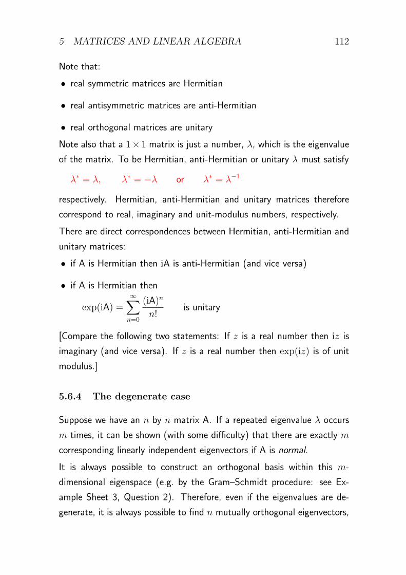
5 MATRICES AND LINEAR ALGEBRA 112

Note that:

• real symmetric matrices are Hermitian

• real antisymmetric matrices are anti-Hermitian

• real orthogonal matrices are unitary

Note also that a 1× 1 matrix is just a number, λ, which is the eigenvalue

of the matrix. To be Hermitian, anti-Hermitian or unitary λ must satisfy

λ∗ = λ, λ∗ = −λ or λ∗ = λ−1

respectively. Hermitian, anti-Hermitian and unitary matrices therefore

correspond to real, imaginary and unit-modulus numbers, respectively.

There are direct correspondences between Hermitian, anti-Hermitian and

unitary matrices:

• if A is Hermitian then iA is anti-Hermitian (and vice versa)

• if A is Hermitian then

exp(iA) =∞∑n=0

(iA)n

n!is unitary

[Compare the following two statements: If z is a real number then iz is

imaginary (and vice versa). If z is a real number then exp(iz) is of unit

modulus.]

5.6.4 The degenerate case

Suppose we have an n by n matrix A. If a repeated eigenvalue λ occurs

m times, it can be shown (with some difficulty) that there are exactly m

corresponding linearly independent eigenvectors if A is normal.

It is always possible to construct an orthogonal basis within this m-

dimensional eigenspace (e.g. by the Gram–Schmidt procedure: see Ex-

ample Sheet 3, Question 2). Therefore, even if the eigenvalues are de-

generate, it is always possible to find n mutually orthogonal eigenvectors,

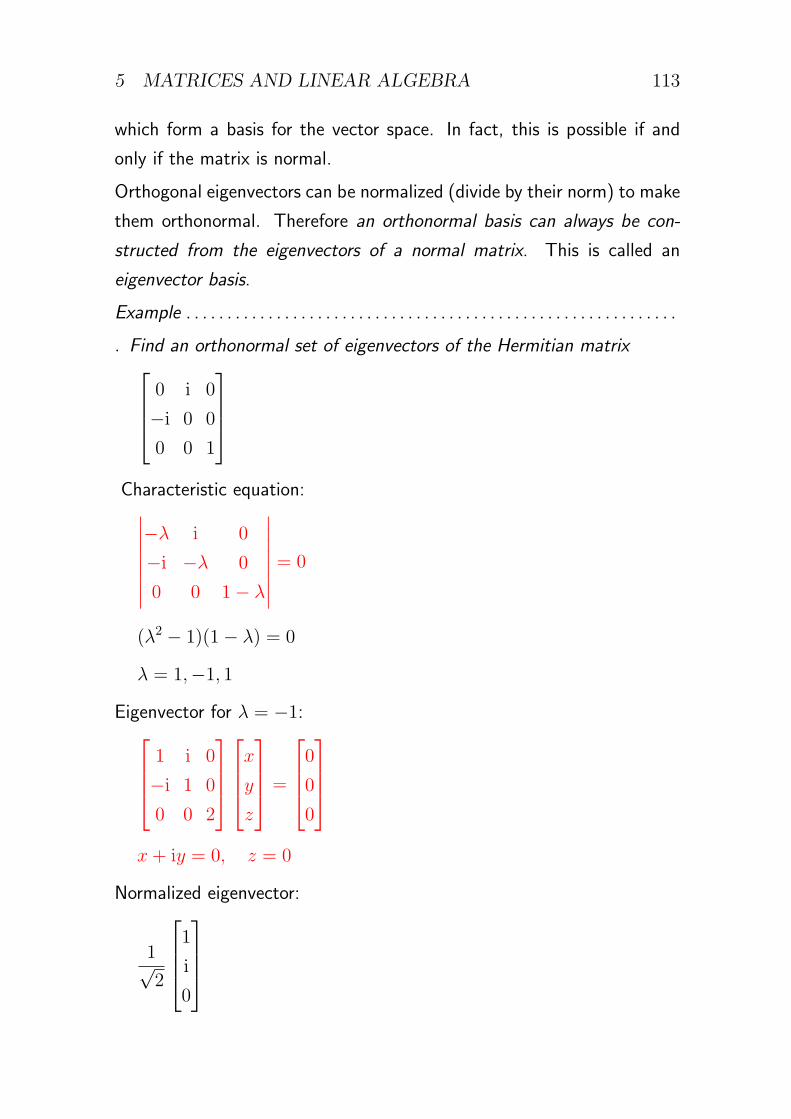
5 MATRICES AND LINEAR ALGEBRA 113

which form a basis for the vector space. In fact, this is possible if and

only if the matrix is normal.

Orthogonal eigenvectors can be normalized (divide by their norm) to make

them orthonormal. Therefore an orthonormal basis can always be con-

structed from the eigenvectors of a normal matrix. This is called an

eigenvector basis.

Example . . . . . . . . . . . . . . . . . . . . . . . . . . . . . . . . . . . . . . . . . . . . . . . . . . . . . . . . . . . .

▷ Find an orthonormal set of eigenvectors of the Hermitian matrix0 i 0

−i 0 0

0 0 1

Characteristic equation:∣∣∣∣∣∣∣∣

−λ i 0

−i −λ 0

0 0 1− λ

∣∣∣∣∣∣∣∣ = 0

(λ2 − 1)(1− λ) = 0

λ = 1,−1, 1

Eigenvector for λ = −1:1 i 0

−i 1 0

0 0 2

x

y

z

=

0

0

0

x+ iy = 0, z = 0

Normalized eigenvector:

1√2

1

i

0

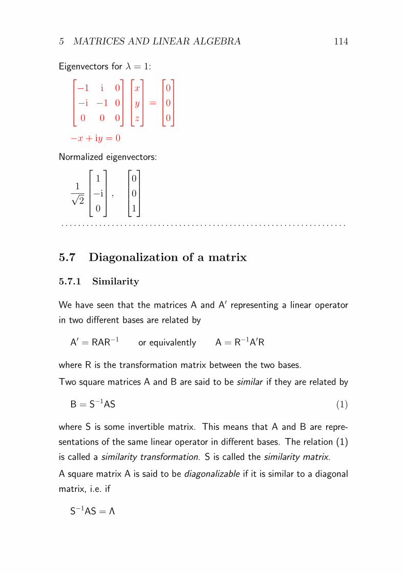
5 MATRICES AND LINEAR ALGEBRA 114

Eigenvectors for λ = 1:−1 i 0

−i −1 0

0 0 0

x

y

z

=

0

0

0

−x+ iy = 0

Normalized eigenvectors:

1√2

1

−i

0

,0

0

1

. . . . . . . . . . . . . . . . . . . . . . . . . . . . . . . . . . . . . . . . . . . . . . . . . . . . . . . . . . . . . . . . . . . .

5.7 Diagonalization of a matrix

5.7.1 Similarity

We have seen that the matrices A and A′ representing a linear operator

in two different bases are related by

A′ = RAR−1 or equivalently A = R−1A′R

where R is the transformation matrix between the two bases.

Two square matrices A and B are said to be similar if they are related by

B = S−1AS (1)

where S is some invertible matrix. This means that A and B are repre-

sentations of the same linear operator in different bases. The relation (1)

is called a similarity transformation. S is called the similarity matrix.

A square matrix A is said to be diagonalizable if it is similar to a diagonal

matrix, i.e. if

S−1AS = Λ

5 MATRICES AND LINEAR ALGEBRA 115

for some invertible matrix S and some diagonal matrix

Λ =

Λ1 0 · · · 0

0 Λ2 · · · 0...

... . . . ...

0 0 · · · Λn

5.7.2 Diagonalization

An n × n matrix A can be diagonalized if and only if it has n linearly

independent eigenvectors. The columns of the similarity matrix S are just

the eigenvectors of A, denoted x(j). The diagonal entries of the matrix Λ

are just the eigenvalues of A, λj:

(S−1AS)ij = (S−1)ikAkℓSℓj

= (S−1)ikAkℓ(x(j))ℓ

= (S−1)ikλj(x(j))k no sum on j

= λj(S−1)ikSkj = λjδij no sum on j

The meaning of diagonalization is that the matrix is expressed in its sim-

plest form by transforming it to its eigenvector basis.

5.7.3 Diagonalization of a normal matrix

An n×n normal matrix always has n linearly independent eigenvectors and

is therefore diagonalizable. Furthermore, the eigenvectors can be chosen

to be orthonormal. In this case the similarity matrix is unitary, because

a unitary matrix is precisely one whose columns are orthonormal vectors

(consider U†U = 1):

(S†S)ij = (S†)ik(S)kj = S∗kiSkj = (x(i))∗k (x

(j))k = (x(i))† x(j) = δij

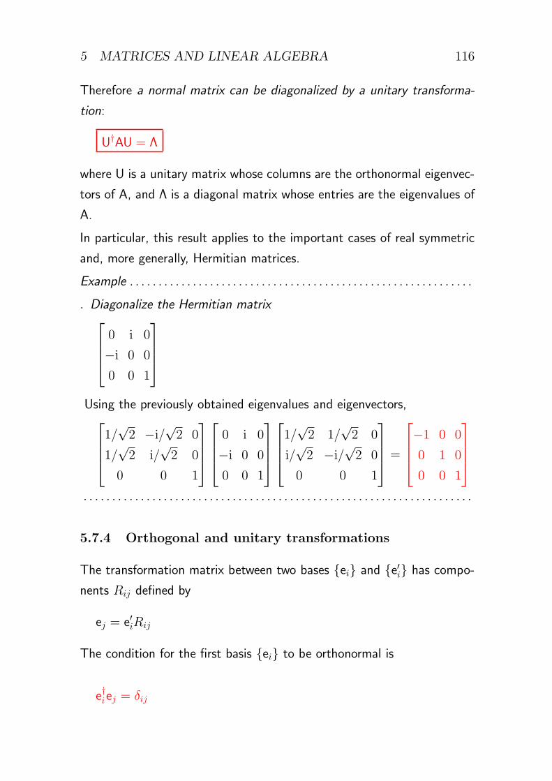
5 MATRICES AND LINEAR ALGEBRA 116

Therefore a normal matrix can be diagonalized by a unitary transforma-

tion:

U†AU = Λ

where U is a unitary matrix whose columns are the orthonormal eigenvec-

tors of A, and Λ is a diagonal matrix whose entries are the eigenvalues of

A.

In particular, this result applies to the important cases of real symmetric

and, more generally, Hermitian matrices.

Example . . . . . . . . . . . . . . . . . . . . . . . . . . . . . . . . . . . . . . . . . . . . . . . . . . . . . . . . . . . .

▷ Diagonalize the Hermitian matrix0 i 0

−i 0 0

0 0 1

Using the previously obtained eigenvalues and eigenvectors,

1/√2 −i/

√2 0

1/√2 i/

√2 0

0 0 1

0 i 0

−i 0 0

0 0 1

1/√2 1/

√2 0

i/√2 −i/

√2 0

0 0 1

=

−1 0 0

0 1 0

0 0 1

. . . . . . . . . . . . . . . . . . . . . . . . . . . . . . . . . . . . . . . . . . . . . . . . . . . . . . . . . . . . . . . . . . . .

5.7.4 Orthogonal and unitary transformations

The transformation matrix between two bases {ei} and {e′i} has compo-

nents Rij defined by

ej = e′iRij

The condition for the first basis {ei} to be orthonormal is

e†iej = δij

5 MATRICES AND LINEAR ALGEBRA 117

(e′kRki)†e′lRlj = δij

R∗kiRlje

′†k e

′l = δij

(In going from the second to the third line, note Rki is a number, so

R†ki = R∗

ki.) If the second basis is also orthonormal, then e′†k e′l = δkl and

the condition becomes

R∗kiRkj = δij

R†R = 1

Therefore the transformation between orthonormal bases is described by

a unitary matrix.

In a real vector space, an orthogonal matrix performs this task. In R2 or

R3 an orthogonal matrix corresponds to a rotation and/or reflection.

A real symmetric matrix is normal and has real eigenvalues and real orthog-

onal eigenvectors. Therefore a real symmetric matrix can be diagonalized

by a real orthogonal transformation.

Note that this is not generally true of real antisymmetric or orthogonal

matrices because their eigenvalues and eigenvectors are not generally real.

They can, however, be diagonalized by complex unitary transformations.

5.7.5 Uses of diagonalization

Certain operations on (diagonalizable) matrices are more easily carried

out using the representation

S−1AS = Λ or A = SΛS−1

Examples:

Am =(SΛS−1

) (SΛS−1

)· · ·

(SΛS−1

)= SΛmS−1

det(A) = det(SΛS−1

)= det(S) det(Λ) det(S−1) = det(Λ)

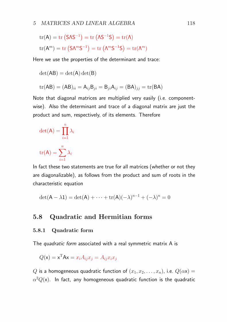
5 MATRICES AND LINEAR ALGEBRA 118

tr(A) = tr(SΛS−1

)= tr

(ΛS−1S

)= tr(Λ)

tr(Am) = tr(SΛmS−1

)= tr

(ΛmS−1S

)= tr(Λm)

Here we use the properties of the determinant and trace:

det(AB) = det(A) det(B)

tr(AB) = (AB)ii = AijBji = BjiAij = (BA)jj = tr(BA)

Note that diagonal matrices are multiplied very easily (i.e. component-

wise). Also the determinant and trace of a diagonal matrix are just the

product and sum, respectively, of its elements. Therefore

det(A) =n∏

i=1

λi

tr(A) =n∑

i=1

λi

In fact these two statements are true for all matrices (whether or not they

are diagonalizable), as follows from the product and sum of roots in the

characteristic equation

det(A− λ1) = det(A) + · · ·+ tr(A)(−λ)n−1 + (−λ)n = 0

5.8 Quadratic and Hermitian forms

5.8.1 Quadratic form

The quadratic form associated with a real symmetric matrix A is

Q(x) = xTAx = xiAijxj = Aijxixj

Q is a homogeneous quadratic function of (x1, x2, . . . , xn), i.e. Q(αx) =

α2Q(x). In fact, any homogeneous quadratic function is the quadratic

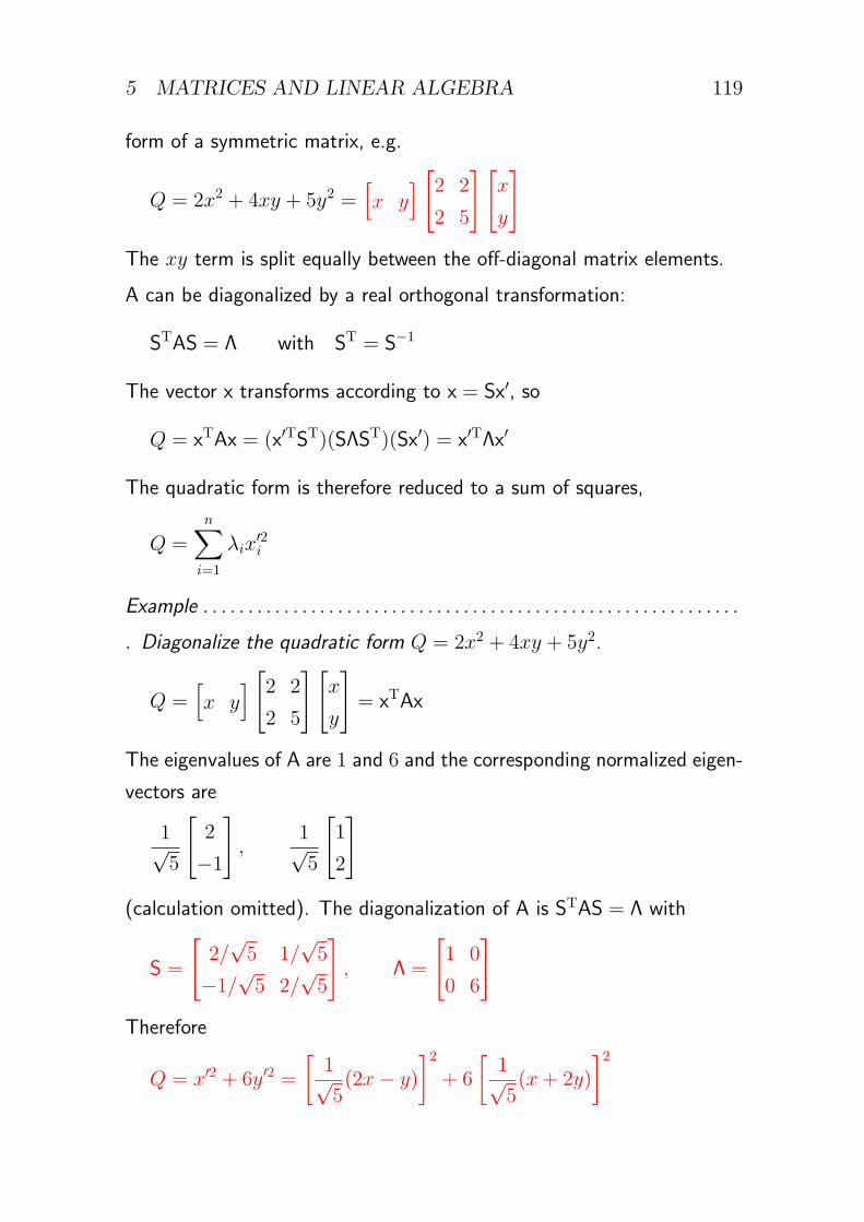
5 MATRICES AND LINEAR ALGEBRA 119

form of a symmetric matrix, e.g.

Q = 2x2 + 4xy + 5y2 =[x y

] [2 2

2 5

][x

y

]The xy term is split equally between the off-diagonal matrix elements.

A can be diagonalized by a real orthogonal transformation:

STAS = Λ with ST = S−1

The vector x transforms according to x = Sx′, so

Q = xTAx = (x′TST)(SΛST)(Sx′) = x′TΛx′

The quadratic form is therefore reduced to a sum of squares,

Q =n∑

i=1

λix′2i

Example . . . . . . . . . . . . . . . . . . . . . . . . . . . . . . . . . . . . . . . . . . . . . . . . . . . . . . . . . . . .

▷ Diagonalize the quadratic form Q = 2x2 + 4xy + 5y2.

Q =[x y

] [2 2

2 5

][x

y

]= xTAx

The eigenvalues of A are 1 and 6 and the corresponding normalized eigen-

vectors are

1√5

[2

−1

],

1√5

[1

2

]

(calculation omitted). The diagonalization of A is STAS = Λ with

S =

[2/√5 1/

√5

−1/√5 2/

√5

], Λ =

[1 0

0 6

]Therefore

Q = x′2 + 6y′2 =

[1√5(2x− y)

]2+ 6

[1√5(x+ 2y)

]2

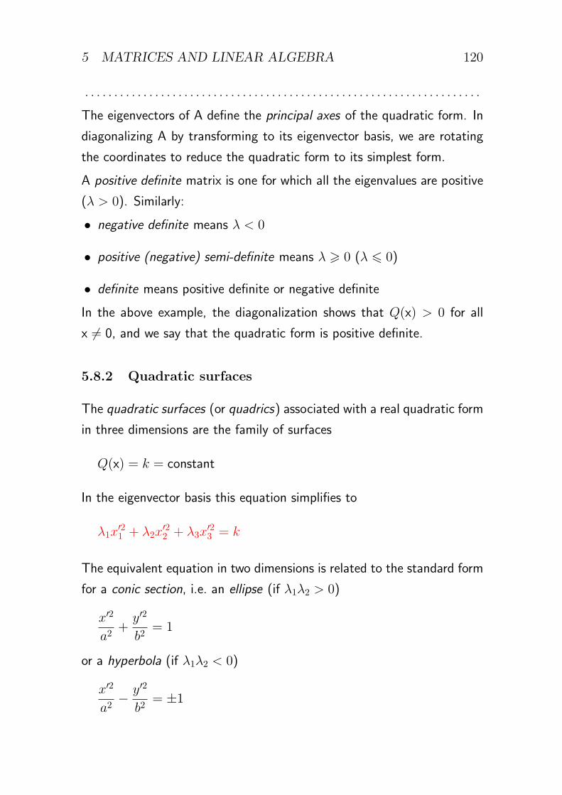
5 MATRICES AND LINEAR ALGEBRA 120

. . . . . . . . . . . . . . . . . . . . . . . . . . . . . . . . . . . . . . . . . . . . . . . . . . . . . . . . . . . . . . . . . . . .

The eigenvectors of A define the principal axes of the quadratic form. In

diagonalizing A by transforming to its eigenvector basis, we are rotating

the coordinates to reduce the quadratic form to its simplest form.

A positive definite matrix is one for which all the eigenvalues are positive

(λ > 0). Similarly:

• negative definite means λ < 0

• positive (negative) semi-definite means λ ⩾ 0 (λ ⩽ 0)

• definite means positive definite or negative definite

In the above example, the diagonalization shows that Q(x) > 0 for all

x = 0, and we say that the quadratic form is positive definite.

5.8.2 Quadratic surfaces

The quadratic surfaces (or quadrics) associated with a real quadratic form

in three dimensions are the family of surfaces

Q(x) = k = constant

In the eigenvector basis this equation simplifies to

λ1x′21 + λ2x

′22 + λ3x

′23 = k

The equivalent equation in two dimensions is related to the standard form

for a conic section, i.e. an ellipse (if λ1λ2 > 0)

x′2

a2+y′2

b2= 1

or a hyperbola (if λ1λ2 < 0)

x′2

a2− y′2

b2= ±1

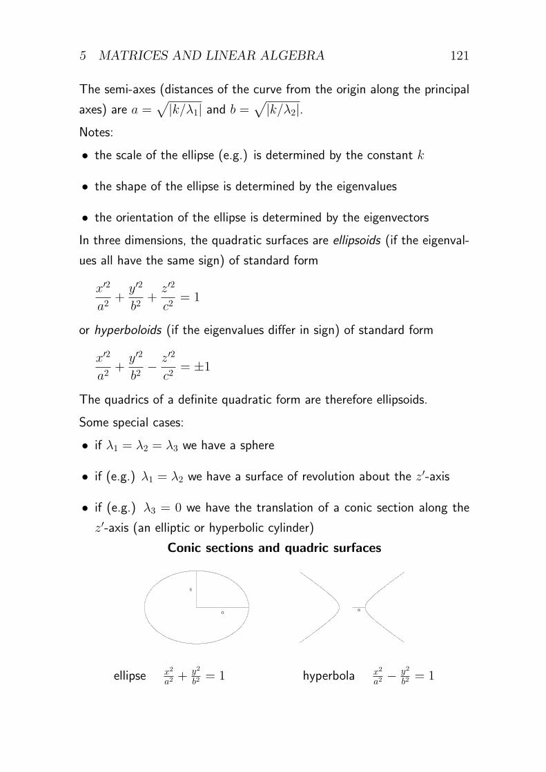
5 MATRICES AND LINEAR ALGEBRA 121

The semi-axes (distances of the curve from the origin along the principal

axes) are a =√

|k/λ1| and b =√

|k/λ2|.

Notes:

• the scale of the ellipse (e.g.) is determined by the constant k

• the shape of the ellipse is determined by the eigenvalues

• the orientation of the ellipse is determined by the eigenvectors

In three dimensions, the quadratic surfaces are ellipsoids (if the eigenval-

ues all have the same sign) of standard form

x′2

a2+y′2

b2+z′2

c2= 1

or hyperboloids (if the eigenvalues differ in sign) of standard form

x′2

a2+y′2

b2− z′2

c2= ±1

The quadrics of a definite quadratic form are therefore ellipsoids.

Some special cases:

• if λ1 = λ2 = λ3 we have a sphere

• if (e.g.) λ1 = λ2 we have a surface of revolution about the z′-axis

• if (e.g.) λ3 = 0 we have the translation of a conic section along the

z′-axis (an elliptic or hyperbolic cylinder)

Conic sections and quadric surfaces

ellipse x2

a2 +y2

b2 = 1 hyperbola x2

a2 −y2

b2 = 1

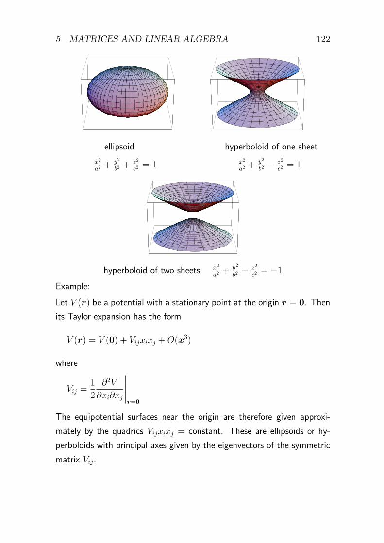
5 MATRICES AND LINEAR ALGEBRA 122

ellipsoid hyperboloid of one sheet

x2

a2 +y2

b2 +z2

c2 = 1 x2

a2 +y2

b2 −z2

c2 = 1

hyperboloid of two sheets x2

a2 +y2

b2 −z2

c2 = −1

Example:

Let V (r) be a potential with a stationary point at the origin r = 0. Then

its Taylor expansion has the form

V (r) = V (0) + Vijxixj +O(x3)

where

Vij =1

2

∂2V

∂xi∂xj

∣∣∣∣∣r=0

The equipotential surfaces near the origin are therefore given approxi-

mately by the quadrics Vijxixj = constant. These are ellipsoids or hy-

perboloids with principal axes given by the eigenvectors of the symmetric

matrix Vij.

5 MATRICES AND LINEAR ALGEBRA 123

5.8.3 Hermitian form

In a complex vector space, the Hermitian form associated with an Hermi-

tian matrix A is

H(x) = x†Ax = x∗iAijxj

H is a real scalar because

H∗ = (x†Ax)† = x†A†x = x†Ax = H

We have seen that A can be diagonalized by a unitary transformation:

U†AU = Λ with U† = U−1

and so

H = x†(UΛU†)x = (U†x)†Λ(U†x) = x′†Λx′ =n∑

i=1

λi|x′i|2 .

5.9 Stationary property of the eigenvalues

The Rayleigh quotient associated with an Hermitian matrix A is the nor-

malized Hermitian form

λ(x) =x†Ax

x†x

Notes:

• λ(x) is a real scalar

• λ(αx) = λ(x)

• if x is an eigenvector of A, then λ(x) is the corresponding eigenvalue

In fact, the eigenvalues of A are the stationary values of the function λ(x).

This is the Rayleigh–Ritz variational principle.

5 MATRICES AND LINEAR ALGEBRA 124

Proof:

δλ = λ(x+ δx)− λ(x)

=(x+ δx)†A(x+ δx)

(x+ δx)†(x+ δx)− λ(x)

=x†Ax+ (δx)†Ax+ x†A(δx) +O(δx2)

x†x+ (δx)†x+ x†(δx) +O(δx2)− λ(x)

=(δx)†Ax+ x†A(δx)− λ(x)[(δx)†x+ x†(δx)] +O(δx2)

x†x+ (δx)†x+ x†(δx) +O(δx2)

=(δx)†[Ax− λ(x)x] + [x†A− λ(x)x†](δx)

x†x+O(δx2)

=(δx)†[Ax− λ(x)x]

x†x+ c.c.+O(δx2)

where ‘c.c.’ denotes the complex conjugate. Therefore the first-order

variation of λ(x) vanishes for all perturbations δx if and only if Ax =

λ(x)x. In that case x is an eigenvector of A, and the value of λ(x) is the

corresponding eigenvalue.

6 ELEMENTARY ANALYSIS 125

6 Elementary analysis

6.1 Motivation

Analysis is the careful study of infinite processes such as limits, conver-

gence, continuity, differential and integral calculus, and is one of the foun-

dations of mathematics. This section covers some of the basic concepts

including the important problem of the convergence of infinite series. It

also introduces the remarkable properties of analytic functions of a com-

plex variable.

6.2 Sequences

6.2.1 Limits of sequences

We first consider a sequence of real or complex numbers fn, defined for

all integers n ⩾ n0. Possible behaviours as n increases are:

• fn tends towards a particular value

• fn does not tend to any value but remains limited in magnitude

• fn is unlimited in magnitude

Definition 1. The sequence fn converges to the limit L as n→ ∞ if,

for any positive number ϵ, |fn − L| < ϵ for sufficiently large n.

In other words the members of the sequence are eventually contained

within an arbitrarily small disk centred on L. We write this as

limn→∞

fn = L or fn → L as n→ ∞

Note that L here is a finite number.

To say that a property holds for sufficiently large n means that there exists

an integer N such that the property is true for all n ⩾ N .

6 ELEMENTARY ANALYSIS 126

Example:

limn→∞

n−α = 0 for any α > 0

Proof:

|n−α − 0| < ϵ holds for all n > ϵ−1/α

If fn does not tend to a limit it may nevertheless be bounded.

Definition 2. The sequence fn is bounded as n→ ∞ if there exists a

positive number K such that |fn| < K for sufficiently large n.

Example:(n+ 1

n

)einα is bounded as n→ ∞ for any real number α

Proof:∣∣∣∣(n+ 1

n

)einα

∣∣∣∣ = n+ 1

n< 2 for all n ⩾ 2

6.2.2 Cauchy’s principle of convergence

A necessary and sufficient condition for the sequence fn to converge is

that, for any positive number ϵ, |fn+m − fn| < ϵ for all positive integers

m, for sufficiently large n. Note that this condition does not require a

knowledge of the value of the limit L.

6 ELEMENTARY ANALYSIS 127

6.3 Convergence of series

6.3.1 Meaning of convergence

What is the meaning of an infinite series such as

∞∑n=n0

un

involving the addition of an infinite number of terms?

We define the partial sum

SN =N∑

n=n0

un

The infinite series∑un is said to converge if the sequence of partial sums

SN tends to a limit S as N → ∞. The value of the series is then S.

Otherwise the series diverges.

Note that whether a series converges or diverges does not depend on the

value of n0 (i.e. on when the series begins) but only on the behaviour of

the terms for large n.

According to Cauchy’s principle of convergence, a necessary and sufficient

condition for∑un to converge is that, for any positive number ϵ,

|SN+m − SN | = |uN+1 + uN+2 + · · ·+ uN+m| < ϵ

for all positive integers m, for sufficiently large N .

6.3.2 Classic examples

The geometric series∑zn has the partial sum

N∑n=0

zn =

1−zN+1

1−z , z = 1

N + 1, z = 1

6 ELEMENTARY ANALYSIS 128

Therefore∑zn converges if |z| < 1, and the sum is 1/(1− z). If |z| ⩾ 1

the series diverges.

The harmonic series∑n−1 diverges. Consider the partial sum

SN =N∑n=1

1

n>

∫ N+1

1

dx

x= ln(N + 1)

Therefore SN increases without bound and does not tend to a limit as

N → ∞.

6.3.3 Absolute and conditional convergence

If∑

|un| converges, then∑un also converges.

∑un is said to converge

absolutely.

If∑

|un| diverges, then∑un may or may not converge. If it does, it is

said to converge conditionally.

[Proof of the first statement above: If∑

|un| converges then, for any

positive number ϵ,

|uN+1|+ |uN+2|+ · · ·+ |uN+m| < ϵ

for all positive integers m, for sufficiently large N . But then

|uN+1 + uN+2 + · · ·+ uN+m| ⩽ |uN+1|+ |uN+2|+ · · ·+ |uN+m|

< ϵ

and so∑un also converges.]

6 ELEMENTARY ANALYSIS 129

6.3.4 Necessary condition for convergence

A necessary condition for∑un to converge is that un → 0 as n → ∞.

Formally, this can be shown by noting that

un = Sn − Sn−1

If the series converges then

limSn = limSn−1 = S

and therefore limun = 0.

This condition is not sufficient for convergence, as exemplified by the

harmonic series.

6.3.5 The comparison test

This refers to series of non-negative real numbers. We write these as

|un| because the comparison test is most often applied in assessing the

absolute convergence of a series of real or complex numbers.

If∑

|vn| converges and

|un| ⩽ |vn| for all n

then∑

|un| also converges. This follows from the fact that

N∑n=n0

|un| ⩽N∑

n=n0

|vn|

and each partial sum is a non-decreasing sequence, which must either

tend to a limit or increase without bound.

More generally, if∑

|vn| converges and

|un| ⩽ K|vn|

for sufficiently large n, whereK is a constant, then∑

|un| also converges.

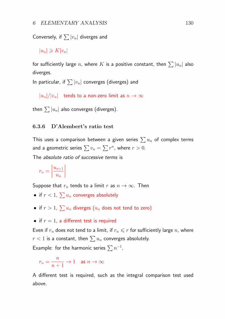
6 ELEMENTARY ANALYSIS 130

Conversely, if∑

|vn| diverges and

|un| ⩾ K|vn|

for sufficiently large n, where K is a positive constant, then∑

|un| alsodiverges.

In particular, if∑

|vn| converges (diverges) and

|un|/|vn| tends to a non-zero limit as n→ ∞

then∑

|un| also converges (diverges).

6.3.6 D’Alembert’s ratio test

This uses a comparison between a given series∑un of complex terms

and a geometric series∑vn =

∑rn, where r > 0.

The absolute ratio of successive terms is

rn =

∣∣∣∣un+1

un

∣∣∣∣Suppose that rn tends to a limit r as n→ ∞. Then

• if r < 1,∑un converges absolutely

• if r > 1,∑un diverges (un does not tend to zero)

• if r = 1, a different test is required

Even if rn does not tend to a limit, if rn ⩽ r for sufficiently large n, where

r < 1 is a constant, then∑un converges absolutely.

Example: for the harmonic series∑n−1,

rn =n

n+ 1→ 1 as n→ ∞

A different test is required, such as the integral comparison test used

above.

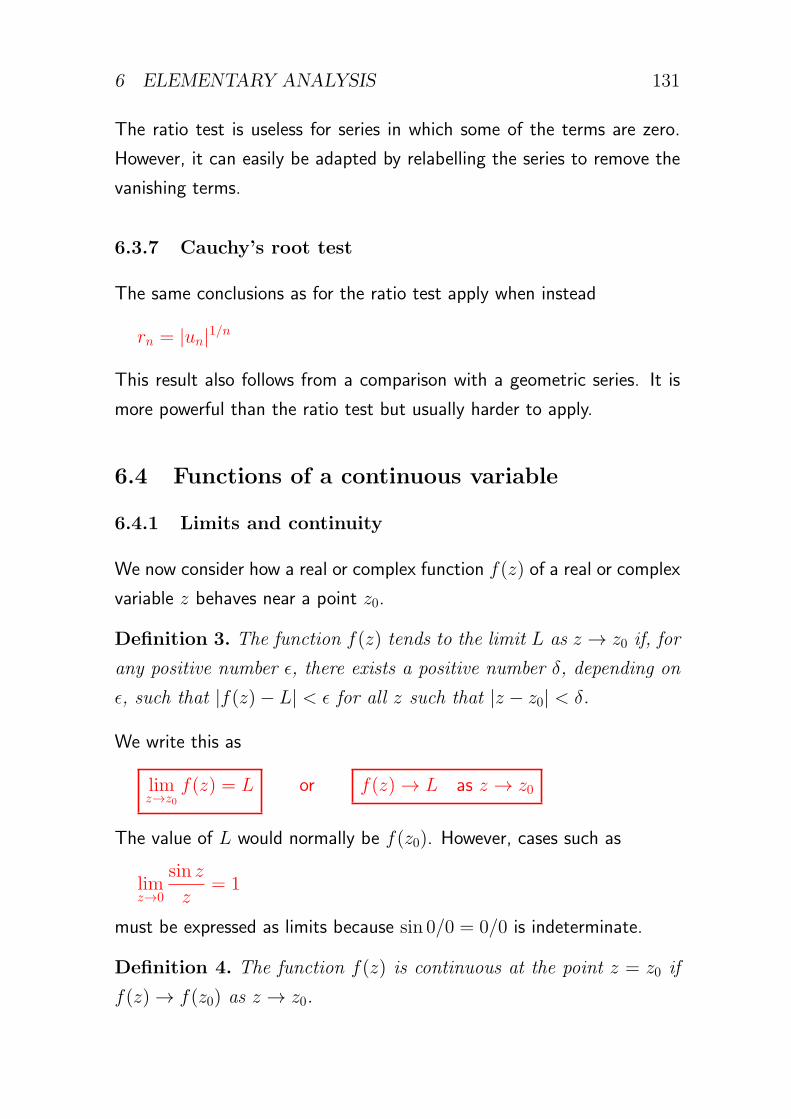
6 ELEMENTARY ANALYSIS 131

The ratio test is useless for series in which some of the terms are zero.

However, it can easily be adapted by relabelling the series to remove the

vanishing terms.

6.3.7 Cauchy’s root test

The same conclusions as for the ratio test apply when instead

rn = |un|1/n

This result also follows from a comparison with a geometric series. It is

more powerful than the ratio test but usually harder to apply.

6.4 Functions of a continuous variable

6.4.1 Limits and continuity

We now consider how a real or complex function f(z) of a real or complex

variable z behaves near a point z0.

Definition 3. The function f(z) tends to the limit L as z → z0 if, for

any positive number ϵ, there exists a positive number δ, depending on

ϵ, such that |f(z)− L| < ϵ for all z such that |z − z0| < δ.

We write this as

limz→z0

f(z) = L or f(z) → L as z → z0

The value of L would normally be f(z0). However, cases such as

limz→0

sin z

z= 1

must be expressed as limits because sin 0/0 = 0/0 is indeterminate.

Definition 4. The function f(z) is continuous at the point z = z0 if

f(z) → f(z0) as z → z0.

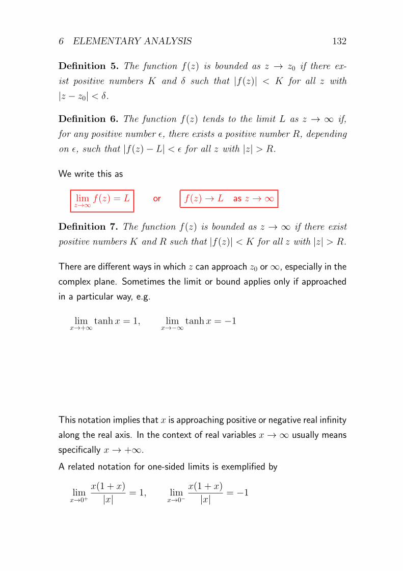
6 ELEMENTARY ANALYSIS 132

Definition 5. The function f(z) is bounded as z → z0 if there ex-

ist positive numbers K and δ such that |f(z)| < K for all z with

|z − z0| < δ.

Definition 6. The function f(z) tends to the limit L as z → ∞ if,

for any positive number ϵ, there exists a positive number R, depending

on ϵ, such that |f(z)− L| < ϵ for all z with |z| > R.

We write this as

limz→∞

f(z) = L or f(z) → L as z → ∞

Definition 7. The function f(z) is bounded as z → ∞ if there exist

positive numbers K and R such that |f(z)| < K for all z with |z| > R.

There are different ways in which z can approach z0 or∞, especially in the

complex plane. Sometimes the limit or bound applies only if approached

in a particular way, e.g.

limx→+∞

tanh x = 1, limx→−∞

tanh x = −1

This notation implies that x is approaching positive or negative real infinity

along the real axis. In the context of real variables x→ ∞ usually means

specifically x→ +∞.

A related notation for one-sided limits is exemplified by

limx→0+

x(1 + x)

|x|= 1, lim

x→0−

x(1 + x)

|x|= −1

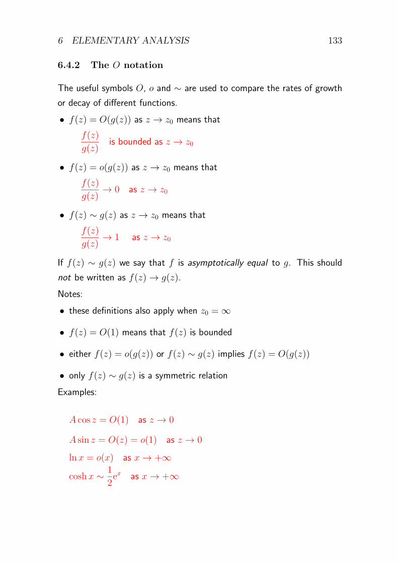
6 ELEMENTARY ANALYSIS 133

6.4.2 The O notation

The useful symbols O, o and ∼ are used to compare the rates of growth

or decay of different functions.

• f(z) = O(g(z)) as z → z0 means that

f(z)

g(z)is bounded as z → z0

• f(z) = o(g(z)) as z → z0 means that

f(z)

g(z)→ 0 as z → z0

• f(z) ∼ g(z) as z → z0 means that

f(z)

g(z)→ 1 as z → z0

If f(z) ∼ g(z) we say that f is asymptotically equal to g. This should

not be written as f(z) → g(z).

Notes:

• these definitions also apply when z0 = ∞

• f(z) = O(1) means that f(z) is bounded

• either f(z) = o(g(z)) or f(z) ∼ g(z) implies f(z) = O(g(z))

• only f(z) ∼ g(z) is a symmetric relation

Examples:

A cos z = O(1) as z → 0

A sin z = O(z) = o(1) as z → 0

lnx = o(x) as x→ +∞

coshx ∼ 1

2ex as x→ +∞

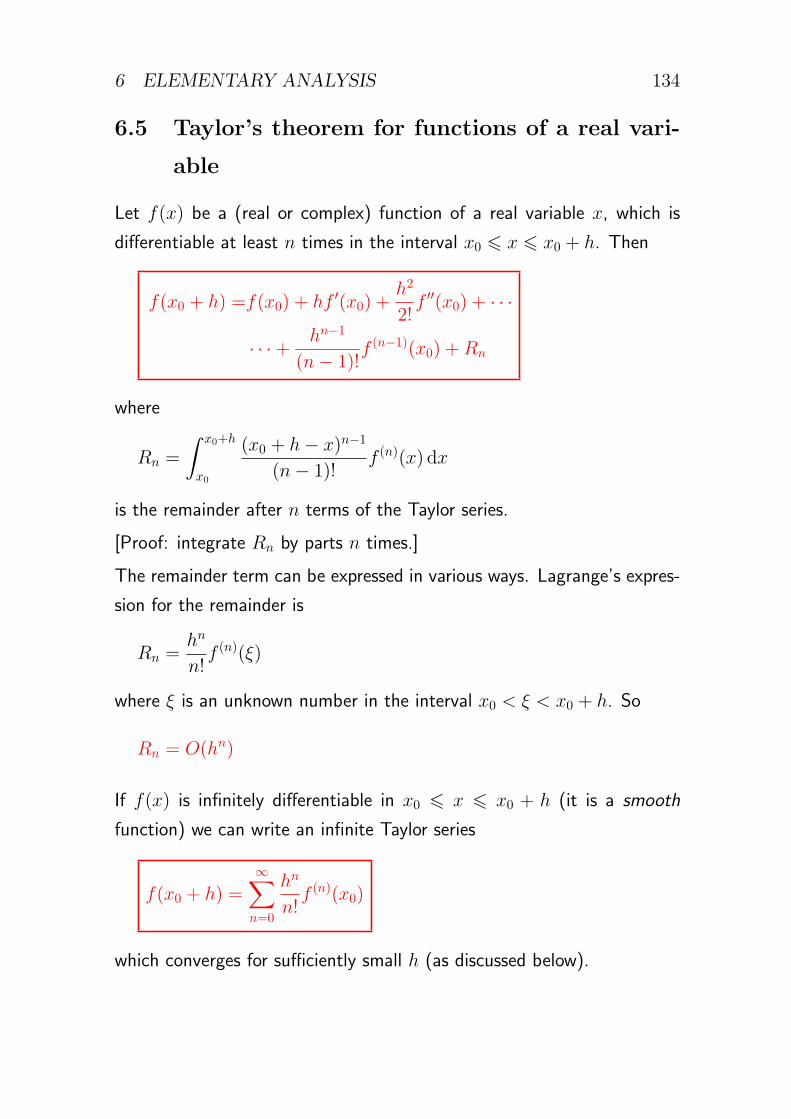
6 ELEMENTARY ANALYSIS 134

6.5 Taylor’s theorem for functions of a real vari-

able

Let f(x) be a (real or complex) function of a real variable x, which is

differentiable at least n times in the interval x0 ⩽ x ⩽ x0 + h. Then

f(x0 + h) =f(x0) + hf ′(x0) +h2

2!f ′′(x0) + · · ·

· · ·+ hn−1

(n− 1)!f (n−1)(x0) +Rn

where

Rn =

∫ x0+h

x0

(x0 + h− x)n−1

(n− 1)!f (n)(x) dx

is the remainder after n terms of the Taylor series.

[Proof: integrate Rn by parts n times.]

The remainder term can be expressed in various ways. Lagrange’s expres-

sion for the remainder is

Rn =hn

n!f (n)(ξ)

where ξ is an unknown number in the interval x0 < ξ < x0 + h. So

Rn = O(hn)

If f(x) is infinitely differentiable in x0 ⩽ x ⩽ x0 + h (it is a smooth

function) we can write an infinite Taylor series

f(x0 + h) =∞∑n=0

hn

n!f (n)(x0)

which converges for sufficiently small h (as discussed below).

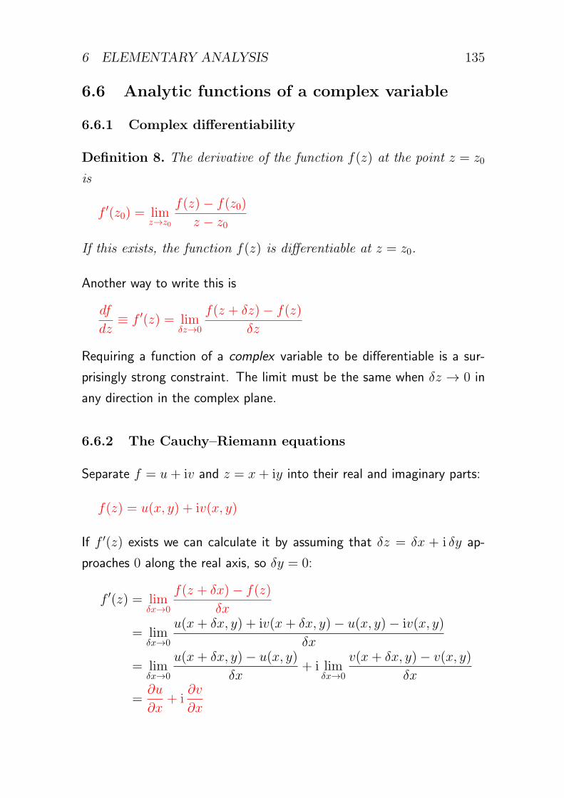
6 ELEMENTARY ANALYSIS 135

6.6 Analytic functions of a complex variable

6.6.1 Complex differentiability

Definition 8. The derivative of the function f(z) at the point z = z0

is

f ′(z0) = limz→z0

f(z)− f(z0)

z − z0

If this exists, the function f(z) is differentiable at z = z0.

Another way to write this is

df

dz≡ f ′(z) = lim

δz→0

f(z + δz)− f(z)

δz

Requiring a function of a complex variable to be differentiable is a sur-

prisingly strong constraint. The limit must be the same when δz → 0 in

any direction in the complex plane.

6.6.2 The Cauchy–Riemann equations

Separate f = u+ iv and z = x+ iy into their real and imaginary parts:

f(z) = u(x, y) + iv(x, y)

If f ′(z) exists we can calculate it by assuming that δz = δx + i δy ap-

proaches 0 along the real axis, so δy = 0:

f ′(z) = limδx→0

f(z + δx)− f(z)

δx

= limδx→0

u(x+ δx, y) + iv(x+ δx, y)− u(x, y)− iv(x, y)

δx

= limδx→0

u(x+ δx, y)− u(x, y)

δx+ i lim

δx→0

v(x+ δx, y)− v(x, y)

δx

=∂u

∂x+ i

∂v

∂x

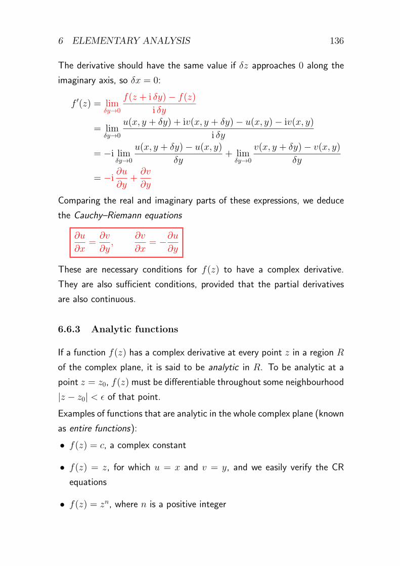
6 ELEMENTARY ANALYSIS 136

The derivative should have the same value if δz approaches 0 along the

imaginary axis, so δx = 0:

f ′(z) = limδy→0

f(z + i δy)− f(z)

i δy

= limδy→0

u(x, y + δy) + iv(x, y + δy)− u(x, y)− iv(x, y)

i δy

= −i limδy→0

u(x, y + δy)− u(x, y)

δy+ lim

δy→0

v(x, y + δy)− v(x, y)

δy

= −i∂u

∂y+∂v

∂y

Comparing the real and imaginary parts of these expressions, we deduce

the Cauchy–Riemann equations

∂u

∂x=∂v

∂y,

∂v

∂x= −∂u

∂y

These are necessary conditions for f(z) to have a complex derivative.

They are also sufficient conditions, provided that the partial derivatives

are also continuous.

6.6.3 Analytic functions

If a function f(z) has a complex derivative at every point z in a region R

of the complex plane, it is said to be analytic in R. To be analytic at a

point z = z0, f(z) must be differentiable throughout some neighbourhood

|z − z0| < ϵ of that point.

Examples of functions that are analytic in the whole complex plane (known

as entire functions):

• f(z) = c, a complex constant

• f(z) = z, for which u = x and v = y, and we easily verify the CR

equations

• f(z) = zn, where n is a positive integer

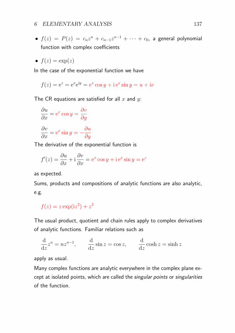
6 ELEMENTARY ANALYSIS 137

• f(z) = P (z) = cnzn + cn−1z

n−1 + · · · + c0, a general polynomial

function with complex coefficients

• f(z) = exp(z)

In the case of the exponential function we have

f(z) = ez = exeiy = ex cos y + i ex sin y = u+ iv

The CR equations are satisfied for all x and y:

∂u

∂x= ex cos y =

∂v

∂y

∂v

∂x= ex sin y = −∂u

∂y

The derivative of the exponential function is

f ′(z) =∂u

∂x+ i

∂v

∂x= ex cos y + i ex sin y = ez

as expected.

Sums, products and compositions of analytic functions are also analytic,

e.g.

f(z) = z exp(iz2) + z3

The usual product, quotient and chain rules apply to complex derivatives

of analytic functions. Familiar relations such as

d

dzzn = nzn−1,

d

dzsin z = cos z,

d

dzcosh z = sinh z

apply as usual.

Many complex functions are analytic everywhere in the complex plane ex-

cept at isolated points, which are called the singular points or singularities

of the function.

6 ELEMENTARY ANALYSIS 138

Examples:

• f(z) = P (z)/Q(z), where P (z) and Q(z) are polynomials. This is

called a rational function and is analytic except at points where Q(z) =

0.

• f(z) = zc, where c is a complex constant, is analytic except at z = 0

(unless c is a non-negative integer)

• f(z) = ln z is also analytic except at z = 0

The last two examples are in fact multiple-valued functions, which require

special treatment (see next term).

Examples of non-analytic functions:

• f(z) = Re(z), for which u = x and v = 0, so the CR equations are

not satisfied anywhere

• f(z) = z∗, for which u = x and v = −y

• f(z) = |z|, for which u = (x2 + y2)1/2 and v = 0

• f(z) = |z|2, for which u = x2 + y2 and v = 0

In the last case the CR equations are satisfied only at x = y = 0 and

we can say that f ′(0) = 0. However, f(z) is not analytic even at z = 0

because it is not differentiable throughout any neighbourhood |z| < ϵ of

0.

6.6.4 Consequences of the Cauchy–Riemann equations

If we know the real part of an analytic function in some region, we can find

its imaginary part (or vice versa) up to an additive constant by integrating

the CR equations.

Example:

u(x, y) = x2 − y2

6 ELEMENTARY ANALYSIS 139

∂v

∂y=∂u

∂x= 2x ⇒ v = 2xy + g(x)

∂v

∂x= −∂u

∂y⇒ 2y + g′(x) = 2y ⇒ g′(x) = 0

Therefore v(x, y) = 2xy+ c, where c is a real constant, and we recognize

f(z) = x2 − y2 + i(2xy + c) = (x+ iy)2 + ic = z2 + ic

The real and imaginary parts of an analytic function satisfy Laplace’s

equation (they are harmonic functions):

∂2u

∂x2+∂2u

∂y2=

∂

∂x

(∂u

∂x

)+

∂

∂y

(∂u

∂y

)=

∂

∂x

(∂v

∂y

)+

∂

∂y

(−∂v∂x

)= 0

The proof that ∇2v = 0 is similar. This provides a useful method for

solving Laplace’s equation in two dimensions. Furthermore,

∇u · ∇v =∂u

∂x

∂v

∂x+∂u

∂y

∂v

∂y

=∂v

∂y

∂v

∂x− ∂v

∂x

∂v

∂y

= 0

and so the curves of constant u and those of constant v intersect at right

angles. u and v are said to be conjugate harmonic functions.

6.7 Taylor series for analytic functions

If a function of a complex variable is analytic in a region R of the complex

plane, not only is it differentiable everywhere in R, it is also differentiable

any number of times. If f(z) is analytic at z = z0, it has an infinite Taylor

6 ELEMENTARY ANALYSIS 140

series

f(z) =∞∑n=0

an(z − z0)n, an =

f (n)(z0)

n!

which converges within some neighbourhood of z0 (as discussed below).

In fact this can be taken as a definition of analyticity.

6.8 Zeros, poles and essential singularities

6.8.1 Zeros of complex functions

The zeros of f(z) are the points z = z0 in the complex plane where

f(z0) = 0. A zero is of order N if

f(z0) = f ′(z0) = f ′′(z0) = · · · = f (N−1)(z0) = 0 but f (N)(z0) = 0

The first non-zero term in the Taylor series of f(z) about z = z0 is then

proportional to (z − z0)N . Indeed

f(z) ∼ aN(z − z0)N as z → z0

A simple zero is a zero of order 1. A double zero is one of order 2, etc.

Examples:

• f(z) = z has a simple zero at z = 0

• f(z) = (z − i)2 has a double zero at z = i

• f(z) = z2 − 1 = (z − 1)(z + 1) has simple zeros at z = ±1

6 ELEMENTARY ANALYSIS 141

Example . . . . . . . . . . . . . . . . . . . . . . . . . . . . . . . . . . . . . . . . . . . . . . . . . . . . . . . . . . . .

▷ Find and classify the zeros of f(z) = sinh z.

0 = sinh z =1

2(ez − e−z)

ez = e−z

e2z = 1

2z = 2nπi

z = nπi, n ∈ Z

f ′(z) = cosh z = cos(nπ) = 0 at these points

⇒ all simple zeros

. . . . . . . . . . . . . . . . . . . . . . . . . . . . . . . . . . . . . . . . . . . . . . . . . . . . . . . . . . . . . . . . . . . .

6.8.2 Poles

Suppose g(z) is analytic and non-zero at z = z0. Consider the function

f(z) = (z − z0)−Ng(z)

Obviously, f(z) is not analytic at z = z0. We say that f(z) has a pole of

order N . Note that

f(z) ∼ g(z0)(z − z0)−N as z → z0 .

A simple pole is a pole of order 1. A double pole is one of order 2, etc.

The behaviour of f(z) near z = z0 can be explored through an expansion

of the following type. Because g(z) is analytic

g(z) =∞∑n=0

bn(z − z0)n with b0 = 0

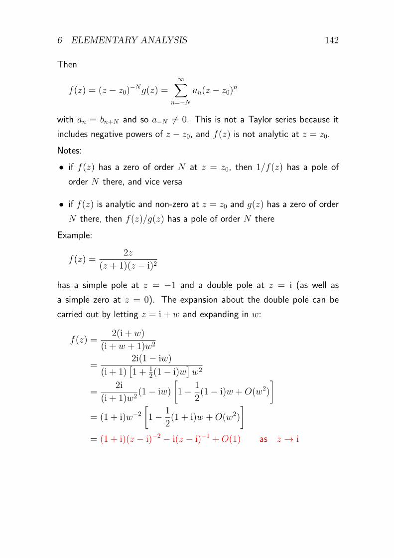
6 ELEMENTARY ANALYSIS 142

Then

f(z) = (z − z0)−Ng(z) =

∞∑n=−N

an(z − z0)n

with an = bn+N and so a−N = 0. This is not a Taylor series because it

includes negative powers of z − z0, and f(z) is not analytic at z = z0.

Notes:

• if f(z) has a zero of order N at z = z0, then 1/f(z) has a pole of

order N there, and vice versa

• if f(z) is analytic and non-zero at z = z0 and g(z) has a zero of order

N there, then f(z)/g(z) has a pole of order N there

Example:

f(z) =2z

(z + 1)(z − i)2

has a simple pole at z = −1 and a double pole at z = i (as well as

a simple zero at z = 0). The expansion about the double pole can be

carried out by letting z = i + w and expanding in w:

f(z) =2(i + w)

(i + w + 1)w2

=2i(1− iw)

(i + 1)[1 + 1

2(1− i)w]w2

=2i

(i + 1)w2(1− iw)

[1− 1

2(1− i)w +O(w2)

]= (1 + i)w−2

[1− 1

2(1 + i)w +O(w2)

]= (1 + i)(z − i)−2 − i(z − i)−1 +O(1) as z → i

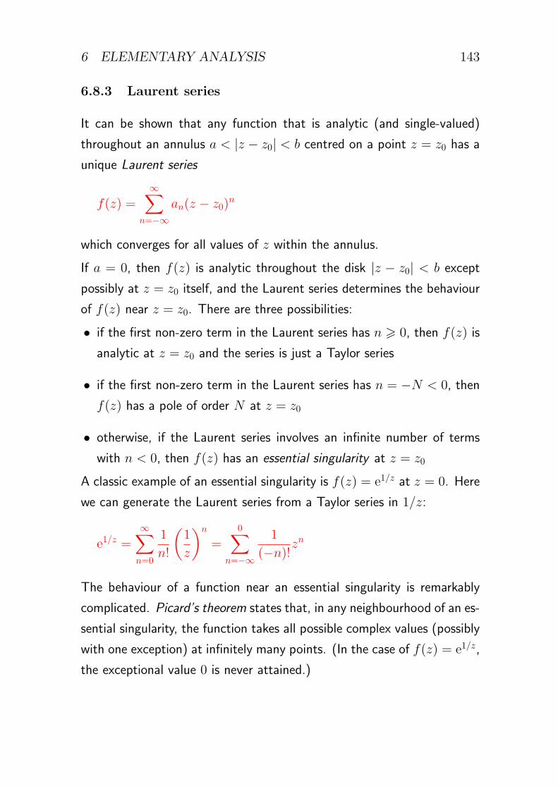
6 ELEMENTARY ANALYSIS 143

6.8.3 Laurent series

It can be shown that any function that is analytic (and single-valued)

throughout an annulus a < |z − z0| < b centred on a point z = z0 has a

unique Laurent series

f(z) =∞∑

n=−∞an(z − z0)

n

which converges for all values of z within the annulus.

If a = 0, then f(z) is analytic throughout the disk |z − z0| < b except

possibly at z = z0 itself, and the Laurent series determines the behaviour

of f(z) near z = z0. There are three possibilities:

• if the first non-zero term in the Laurent series has n ⩾ 0, then f(z) is

analytic at z = z0 and the series is just a Taylor series

• if the first non-zero term in the Laurent series has n = −N < 0, then

f(z) has a pole of order N at z = z0

• otherwise, if the Laurent series involves an infinite number of terms

with n < 0, then f(z) has an essential singularity at z = z0

A classic example of an essential singularity is f(z) = e1/z at z = 0. Here

we can generate the Laurent series from a Taylor series in 1/z:

e1/z =∞∑n=0

1

n!

(1

z

)n

=0∑

n=−∞

1

(−n)!zn

The behaviour of a function near an essential singularity is remarkably

complicated. Picard’s theorem states that, in any neighbourhood of an es-

sential singularity, the function takes all possible complex values (possibly

with one exception) at infinitely many points. (In the case of f(z) = e1/z,

the exceptional value 0 is never attained.)

6 ELEMENTARY ANALYSIS 144

6.8.4 Behaviour at infinity

We can examine the behaviour of a function f(z) as z → ∞ by defining

a new variable ζ = 1/z and a new function g(ζ) = f(z). Then z = ∞maps to a single point ζ = 0, the point at infinity.

If g(ζ) has a zero, pole or essential singularity at ζ = 0, then we can say

that f(z) has the corresponding property at z = ∞.

Examples:

f1(z) = ez = e1/ζ = g1(ζ)

has an essential singularity at z = ∞.

f2(z) = z2 = 1/ζ2 = g2(ζ)

has a double pole at z = ∞.

f3(z) = e1/z = eζ = g3(ζ)

is analytic at z = ∞.

6.9 Convergence of power series

6.9.1 Circle of convergence

If the power series

f(z) =∞∑n=0

an(z − z0)n

converges for z = z1, then the series converges absolutely for all z such

that |z − z0| < |z1 − z0|.

[Proof: The necessary condition for convergence,

limn→∞

an(z1 − z0)n = 0

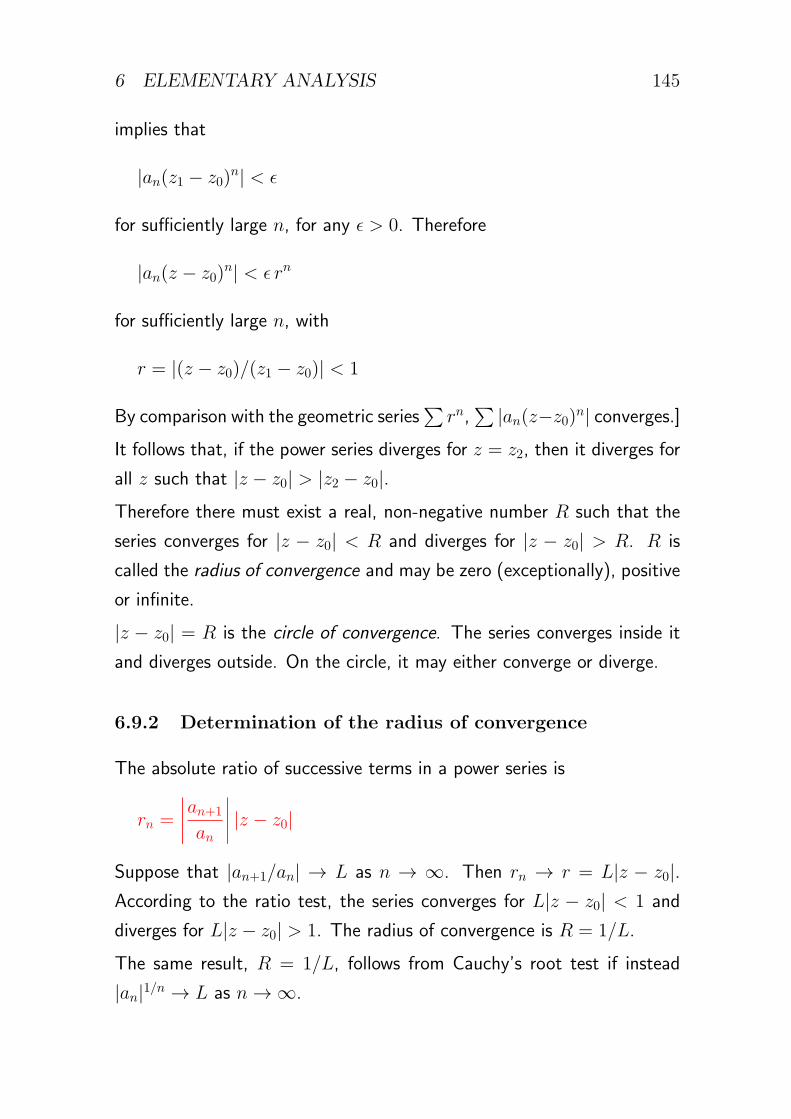
6 ELEMENTARY ANALYSIS 145

implies that

|an(z1 − z0)n| < ϵ

for sufficiently large n, for any ϵ > 0. Therefore

|an(z − z0)n| < ϵ rn

for sufficiently large n, with

r = |(z − z0)/(z1 − z0)| < 1

By comparison with the geometric series∑rn,

∑|an(z−z0)n| converges.]

It follows that, if the power series diverges for z = z2, then it diverges for

all z such that |z − z0| > |z2 − z0|.

Therefore there must exist a real, non-negative number R such that the

series converges for |z − z0| < R and diverges for |z − z0| > R. R is

called the radius of convergence and may be zero (exceptionally), positive

or infinite.

|z − z0| = R is the circle of convergence. The series converges inside it

and diverges outside. On the circle, it may either converge or diverge.

6.9.2 Determination of the radius of convergence

The absolute ratio of successive terms in a power series is

rn =

∣∣∣∣an+1

an

∣∣∣∣ |z − z0|

Suppose that |an+1/an| → L as n → ∞. Then rn → r = L|z − z0|.According to the ratio test, the series converges for L|z − z0| < 1 and

diverges for L|z − z0| > 1. The radius of convergence is R = 1/L.

The same result, R = 1/L, follows from Cauchy’s root test if instead

|an|1/n → L as n→ ∞.

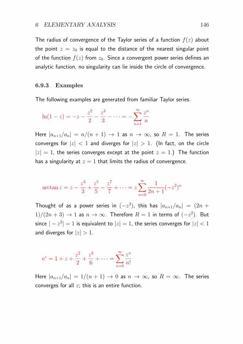
6 ELEMENTARY ANALYSIS 146

The radius of convergence of the Taylor series of a function f(z) about

the point z = z0 is equal to the distance of the nearest singular point

of the function f(z) from z0. Since a convergent power series defines an

analytic function, no singularity can lie inside the circle of convergence.

6.9.3 Examples

The following examples are generated from familiar Taylor series.

ln(1− z) = −z − z2

2− z3

3− · · · = −

∞∑n=1

zn

n

Here |an+1/an| = n/(n + 1) → 1 as n → ∞, so R = 1. The series

converges for |z| < 1 and diverges for |z| > 1. (In fact, on the circle

|z| = 1, the series converges except at the point z = 1.) The function

has a singularity at z = 1 that limits the radius of convergence.

arctan z = z − z3

3+z5

5− z7

7+ · · · = z

∞∑n=0

1

2n+ 1(−z2)n

Thought of as a power series in (−z2), this has |an+1/an| = (2n +

1)/(2n + 3) → 1 as n → ∞. Therefore R = 1 in terms of (−z2). But

since | − z2| = 1 is equivalent to |z| = 1, the series converges for |z| < 1

and diverges for |z| > 1.

ez = 1 + z +z2

2+z3

6+ · · · =

∞∑n=0

zn

n!

Here |an+1/an| = 1/(n + 1) → 0 as n → ∞, so R = ∞. The series

converges for all z; this is an entire function.

7 ORDINARY DIFFERENTIAL EQUATIONS 147

7 Ordinary differential equations

7.1 Motivation

Very many scientific problems are described by differential equations. Even

if these are partial differential equations, they can often be reduced to

ordinary differential equations (ODEs), e.g. by the method of separation

of variables.

The ODEs encountered most frequently are linear and of either first or

second order. In particular, second-order equations describe oscillatory

phenomena.

Part IA dealt with first-order ODEs and also with linear second-order ODEs

with constant coefficients. Here we deal with general linear second-order

ODEs.

The general linear inhomogeneous first-order ODE

y′(x) + p(x)y(x) = f(x)

can be solved using the integrating factor

g = exp

∫p(x) dx

to obtain the general solution

y =1

g

∫gf dx

Provided that the integrals can be evaluated, the problem is completely

solved. An equivalent method does not exist for second-order ODEs, but

an extensive theory can still be developed.

7.2 Classification

The general second-order ODE is an equation of the form

F (y′′, y′, y, x) = 0

7 ORDINARY DIFFERENTIAL EQUATIONS 148

for an unknown function y(x), where y′ = dy/dx and y′′ = d2y/dx2.

The general linear second-order ODE has the form

Ly = f

where L is a linear operator such that

Ly = ay′′ + by′ + cy

where a, b, c, f are functions of x.

The equation is homogeneous (unforced) if f = 0, otherwise it is inho-

mogeneous (forced).

The principle of superposition applies to linear ODEs as to all linear equa-

tions.

Although the solution may be of interest only for real x, it is often infor-

mative to analyse the solution in the complex domain.

7.3 Homogeneous linear second-order ODEs

7.3.1 Linearly independent solutions

Divide through by the coefficient of y′′ to obtain a standard form

y′′(x) + p(x)y′(x) + q(x)y(x) = 0

Suppose that y1(x) and y2(x) are two solutions of this equation. They

are linearly independent if

Ay1(x) +By2(x) = 0 (for all x) implies A = B = 0

i.e. if one is not simply a constant multiple of the other.

If y1(x) and y2(x) are linearly independent solutions, then the general

solution of the ODE is

y(x) = Ay1(x) +By2(x)

7 ORDINARY DIFFERENTIAL EQUATIONS 149

where A and B are arbitrary constants. There are two arbitrary constants

because the equation is of second order.

7.3.2 The Wronskian

The Wronskian W (x) of two solutions y1(x) and y2(x) of a second-order

ODE is the determinant of the Wronskian matrix:

W [y1, y2] =

∣∣∣∣∣y1 y2

y′1 y′2

∣∣∣∣∣ = y1y′2 − y2y

′1

Suppose that Ay1(x) + By2(x) = 0 in some interval of x. Then also

Ay′1(x) +By′2(x) = 0, and so[y1 y2

y′1 y′2

][A

B

]=

[0

0

]If this is satisfied for non-trivial A, B then W = 0 (in that interval of x).

Therefore the solutions are linearly independent if W = 0.

7.3.3 Calculation of the Wronskian

Consider

W ′ = y1y′′2 − y2y

′′1

= y1(−py′2 − qy2)− y2(−py′1 − qy1)

= −pW

since both y1 and y2 solve the ODE. This first-order ODE for W has the

solution

W = exp

(−∫p dx

)This expression involves an indefinite integral and could be written as

W (x) = exp

[−∫ x

p(ξ) dξ

]

7 ORDINARY DIFFERENTIAL EQUATIONS 150

Notes:

• the indefinite integral involves an arbitrary additive constant, so W

involves an arbitrary multiplicative constant

• apart from that, W is the same for any two solutions y1 and y2

• W is therefore an intrinsic property of the ODE

• if W = 0 for one value of x (and p is integrable) then W = 0 for all

x, so linear independence need be checked at only one value of x

7.3.4 Finding a second solution

Suppose that one solution y1(x) is known. Then a second solution y2(x)

can be found as follows.

First find W as described above. The definition of W then provides a

first-order linear ODE for the unknown y2:

y1y′2 − y2y

′1 = W

y′2y1

− y2y′1

y21=W

y21

d

dx

(y2y1

)=W

y21

y2 = y1

∫W

y21dx

Again, this result involves an indefinite integral and could be written as

y2(x) = y1(x)

∫ x W (ξ)

[y1(ξ)]2dξ

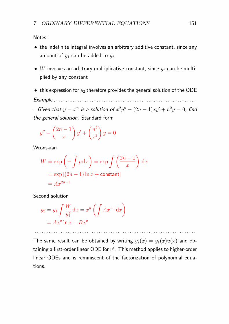
7 ORDINARY DIFFERENTIAL EQUATIONS 151

Notes:

• the indefinite integral involves an arbitrary additive constant, since any

amount of y1 can be added to y2

• W involves an arbitrary multiplicative constant, since y2 can be multi-

plied by any constant

• this expression for y2 therefore provides the general solution of the ODE

Example . . . . . . . . . . . . . . . . . . . . . . . . . . . . . . . . . . . . . . . . . . . . . . . . . . . . . . . . . . . .

▷ Given that y = xn is a solution of x2y′′ − (2n− 1)xy′ + n2y = 0, find

the general solution. Standard form

y′′ −(2n− 1

x

)y′ +

(n2

x2

)y = 0

Wronskian

W = exp

(−∫p dx

)= exp

∫ (2n− 1

x

)dx

= exp [(2n− 1) ln x+ constant]

= Ax2n−1

Second solution

y2 = y1

∫W

y21dx = xn

(∫Ax−1 dx

)= Axn lnx+Bxn

. . . . . . . . . . . . . . . . . . . . . . . . . . . . . . . . . . . . . . . . . . . . . . . . . . . . . . . . . . . . . . . . . . . .

The same result can be obtained by writing y2(x) = y1(x)u(x) and ob-

taining a first-order linear ODE for u′. This method applies to higher-order

linear ODEs and is reminiscent of the factorization of polynomial equa-

tions.

7 ORDINARY DIFFERENTIAL EQUATIONS 152

7.4 Series solutions

7.4.1 Ordinary and singular points

We consider a homogeneous linear second-order ODE in standard form:

y′′(x) + p(x)y′(x) + q(x)y(x) = 0

A point x = x0 is an ordinary point of the ODE if:

p(x) and q(x) are both analytic at x = x0

Otherwise it is a singular point.

A singular point x = x0 is regular if:

(x− x0)p(x) and (x− x0)2q(x) are both analytic at x = x0

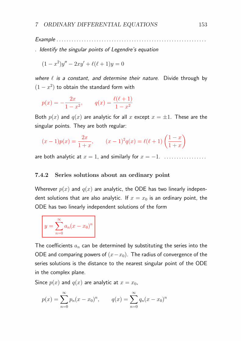
7 ORDINARY DIFFERENTIAL EQUATIONS 153

Example . . . . . . . . . . . . . . . . . . . . . . . . . . . . . . . . . . . . . . . . . . . . . . . . . . . . . . . . . . . .

▷ Identify the singular points of Legendre’s equation

(1− x2)y′′ − 2xy′ + ℓ(ℓ+ 1)y = 0

where ℓ is a constant, and determine their nature. Divide through by

(1− x2) to obtain the standard form with

p(x) = − 2x

1− x2, q(x) =

ℓ(ℓ+ 1)

1− x2

Both p(x) and q(x) are analytic for all x except x = ±1. These are the

singular points. They are both regular:

(x− 1)p(x) =2x

1 + x, (x− 1)2q(x) = ℓ(ℓ+ 1)

(1− x

1 + x

)are both analytic at x = 1, and similarly for x = −1. . . . . . . . . . . . . . . . . .

7.4.2 Series solutions about an ordinary point

Wherever p(x) and q(x) are analytic, the ODE has two linearly indepen-

dent solutions that are also analytic. If x = x0 is an ordinary point, the

ODE has two linearly independent solutions of the form

y =∞∑n=0

an(x− x0)n

The coefficients an can be determined by substituting the series into the

ODE and comparing powers of (x−x0). The radius of convergence of theseries solutions is the distance to the nearest singular point of the ODE

in the complex plane.

Since p(x) and q(x) are analytic at x = x0,

p(x) =∞∑n=0

pn(x− x0)n, q(x) =

∞∑n=0

qn(x− x0)n

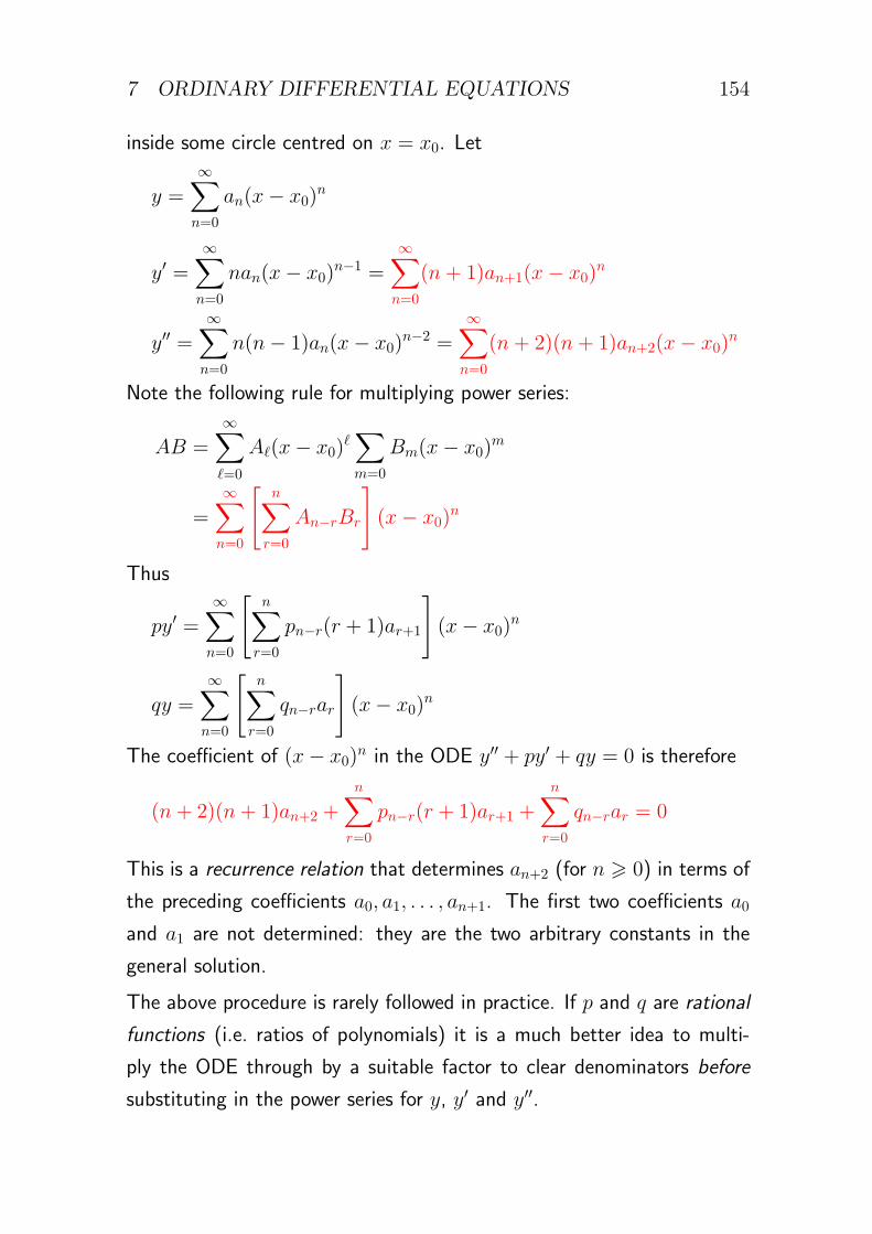
7 ORDINARY DIFFERENTIAL EQUATIONS 154

inside some circle centred on x = x0. Let

y =∞∑n=0

an(x− x0)n

y′ =∞∑n=0

nan(x− x0)n−1 =

∞∑n=0

(n+ 1)an+1(x− x0)n

y′′ =∞∑n=0

n(n− 1)an(x− x0)n−2 =

∞∑n=0

(n+ 2)(n+ 1)an+2(x− x0)n

Note the following rule for multiplying power series:

AB =∞∑ℓ=0

Aℓ(x− x0)ℓ∑m=0

Bm(x− x0)m

=∞∑n=0

[n∑

r=0

An−rBr

](x− x0)

n

Thus

py′ =∞∑n=0

[n∑

r=0

pn−r(r + 1)ar+1

](x− x0)

n

qy =∞∑n=0

[n∑

r=0

qn−rar

](x− x0)

n

The coefficient of (x− x0)n in the ODE y′′ + py′ + qy = 0 is therefore

(n+ 2)(n+ 1)an+2 +n∑

r=0

pn−r(r + 1)ar+1 +n∑

r=0

qn−rar = 0

This is a recurrence relation that determines an+2 (for n ⩾ 0) in terms of

the preceding coefficients a0, a1, . . . , an+1. The first two coefficients a0

and a1 are not determined: they are the two arbitrary constants in the

general solution.

The above procedure is rarely followed in practice. If p and q are rational

functions (i.e. ratios of polynomials) it is a much better idea to multi-

ply the ODE through by a suitable factor to clear denominators before

substituting in the power series for y, y′ and y′′.

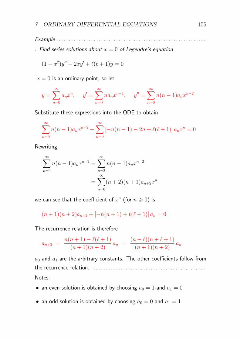
7 ORDINARY DIFFERENTIAL EQUATIONS 155

Example . . . . . . . . . . . . . . . . . . . . . . . . . . . . . . . . . . . . . . . . . . . . . . . . . . . . . . . . . . . .

▷ Find series solutions about x = 0 of Legendre’s equation

(1− x2)y′′ − 2xy′ + ℓ(ℓ+ 1)y = 0

x = 0 is an ordinary point, so let

y =∞∑n=0

anxn, y′ =

∞∑n=0

nanxn−1, y′′ =

∞∑n=0

n(n− 1)anxn−2

Substitute these expressions into the ODE to obtain

∞∑n=0

n(n− 1)anxn−2 +

∞∑n=0

[−n(n− 1)− 2n+ ℓ(ℓ+ 1)] anxn = 0

Rewriting

∞∑n=0

n(n− 1)anxn−2 =

∞∑n=2

n(n− 1)anxn−2

=∞∑n=0

(n+ 2)(n+ 1)an+2xn

we can see that the coefficient of xn (for n ⩾ 0) is

(n+ 1)(n+ 2)an+2 + [−n(n+ 1) + ℓ(ℓ+ 1)] an = 0

The recurrence relation is therefore

an+2 =n(n+ 1)− ℓ(ℓ+ 1)

(n+ 1)(n+ 2)an =

(n− ℓ)(n+ ℓ+ 1)

(n+ 1)(n+ 2)an

a0 and a1 are the arbitrary constants. The other coefficients follow from

the recurrence relation. . . . . . . . . . . . . . . . . . . . . . . . . . . . . . . . . . . . . . . . . . . . . .

Notes:

• an even solution is obtained by choosing a0 = 1 and a1 = 0

• an odd solution is obtained by choosing a0 = 0 and a1 = 1

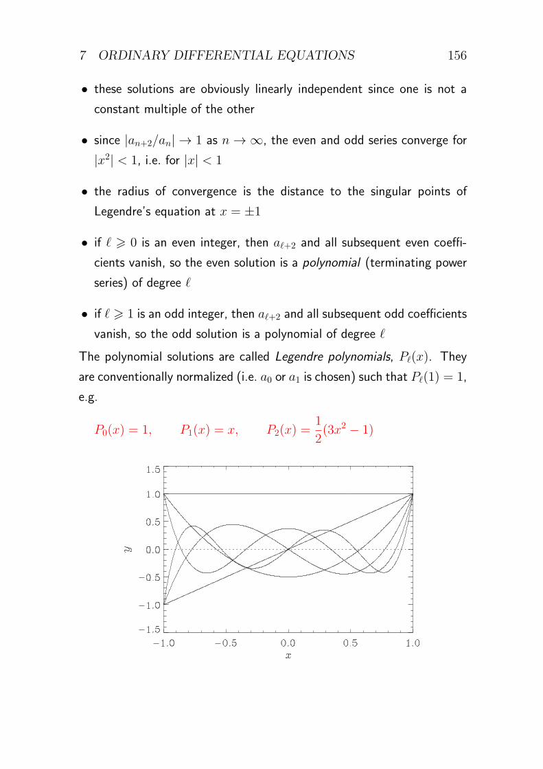
7 ORDINARY DIFFERENTIAL EQUATIONS 156

• these solutions are obviously linearly independent since one is not a

constant multiple of the other

• since |an+2/an| → 1 as n → ∞, the even and odd series converge for

|x2| < 1, i.e. for |x| < 1

• the radius of convergence is the distance to the singular points of

Legendre’s equation at x = ±1

• if ℓ ⩾ 0 is an even integer, then aℓ+2 and all subsequent even coeffi-

cients vanish, so the even solution is a polynomial (terminating power

series) of degree ℓ

• if ℓ ⩾ 1 is an odd integer, then aℓ+2 and all subsequent odd coefficients

vanish, so the odd solution is a polynomial of degree ℓ

The polynomial solutions are called Legendre polynomials, Pℓ(x). They

are conventionally normalized (i.e. a0 or a1 is chosen) such that Pℓ(1) = 1,

e.g.

P0(x) = 1, P1(x) = x, P2(x) =1

2(3x2 − 1)

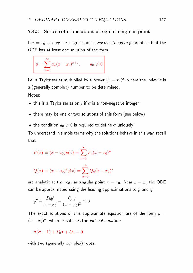
7 ORDINARY DIFFERENTIAL EQUATIONS 157

7.4.3 Series solutions about a regular singular point

If x = x0 is a regular singular point, Fuchs’s theorem guarantees that the

ODE has at least one solution of the form

y =∞∑n=0

an(x− x0)n+σ, a0 = 0

i.e. a Taylor series multiplied by a power (x− x0)σ, where the index σ is

a (generally complex) number to be determined.

Notes:

• this is a Taylor series only if σ is a non-negative integer

• there may be one or two solutions of this form (see below)

• the condition a0 = 0 is required to define σ uniquely

To understand in simple terms why the solutions behave in this way, recall

that

P (x) ≡ (x− x0)p(x) =∞∑n=0

Pn(x− x0)n

Q(x) ≡ (x− x0)2q(x) =

∞∑n=0

Qn(x− x0)n

are analytic at the regular singular point x = x0. Near x = x0 the ODE

can be approximated using the leading approximations to p and q:

y′′ +P0y

′

x− x0+

Q0y

(x− x0)2≈ 0

The exact solutions of this approximate equation are of the form y =

(x− x0)σ, where σ satisfies the indicial equation

σ(σ − 1) + P0σ +Q0 = 0

with two (generally complex) roots.

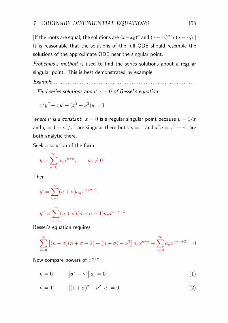
7 ORDINARY DIFFERENTIAL EQUATIONS 158

[If the roots are equal, the solutions are (x−x0)σ and (x−x0)σ ln(x−x0).]It is reasonable that the solutions of the full ODE should resemble the

solutions of the approximate ODE near the singular point.

Frobenius’s method is used to find the series solutions about a regular

singular point. This is best demonstrated by example.

Example . . . . . . . . . . . . . . . . . . . . . . . . . . . . . . . . . . . . . . . . . . . . . . . . . . . . . . . . . . . .

▷ Find series solutions about x = 0 of Bessel’s equation

x2y′′ + xy′ + (x2 − ν2)y = 0

where ν is a constant. x = 0 is a regular singular point because p = 1/x

and q = 1− ν2/x2 are singular there but xp = 1 and x2q = x2 − ν2 are

both analytic there.

Seek a solution of the form

y =∞∑n=0

anxn+σ, a0 = 0

Then

y′ =∞∑n=0

(n+ σ)anxn+σ−1,

y′′ =∞∑n=0

(n+ σ)(n+ σ − 1)anxn+σ−2

Bessel’s equation requires

∞∑n=0

[(n+ σ)(n+ σ − 1) + (n+ σ)− ν2

]anx

n+σ +∞∑n=0

anxn+σ+2 = 0

Now compare powers of xn+σ:

n = 0 :[σ2 − ν2

]a0 = 0 (1)

n = 1 :[(1 + σ)2 − ν2

]a1 = 0 (2)

7 ORDINARY DIFFERENTIAL EQUATIONS 159

n ⩾ 2 :[(n+ σ)2 − ν2

]an + an−2 = 0 (3)

Since a0 = 0 by assumption, equation (1) provides the indicial equation

σ2 − ν2 = 0

with roots σ = ±ν. Equation (2) then requires that a1 = 0 (except

possibly in the case ν = ±12 , but even then a1 can be chosen to be 0).

Equation (3) provides the recurrence relation

an = − an−2

n(n+ 2σ)

Since a1 = 0, all the odd coefficients vanish. Since |an/an−2| → 0 as

n→ ∞, the radius of convergence of the series is infinite.

For most values of ν we therefore obtain two linearly independent solutions

(choosing a0 = 1):

y1 = xν[1− x2

4(1 + ν)+

x4

32(1 + ν)(2 + ν)+ · · ·

]

y2 = x−ν

[1− x2

4(1− ν)+

x4

32(1− ν)(2− ν)+ · · ·

]However, if ν = 0 there is clearly only one solution of this form. Further-

more, if ν is a non-zero integer one of the recurrence relations will fail

at some point and the corresponding series is invalid. In these cases the

second solution is of a different form (see below). . . . . . . . . . . . . . . . . . . . .

A general analysis shows that:

• if the roots of the indicial equation are equal, there is only one solution

of the form∑an(x− x0)

n+σ

• if the roots differ by an integer, there is generally only one solution

of this form because the recurrence relation for the smaller value of

Re(σ) will usually (but not always) fail

• otherwise, there are two solutions of the form∑an(x− x0)

n+σ

7 ORDINARY DIFFERENTIAL EQUATIONS 160

• the radius of convergence of the series is the distance from the point

of expansion to the nearest singular point of the ODE

If the roots σ1, σ2 of the indicial equation are equal or differ by an integer,

one solution is of the form

y1 =∞∑n=0

an(x− x0)n+σ1, Re(σ1) ⩾ Re(σ2)

and the other is of the form

y2 =∞∑n=0

bn(x− x0)n+σ2 + cy1 ln(x− x0)

The coefficients bn and c can be determined (with some difficulty) by

substituting this form into the ODE and comparing coefficients of (x−x0)n

and (x− x0)n ln(x− x0). In exceptional cases c may vanish.

Alternatively, y2 can be found (also with some difficulty) using the Wron-

skian method (section 7.3.4).

Example: Bessel’s equation of order ν = 0:

y1 = 1− x2

4+x4

64+ · · ·

y2 = y1 lnx+x2

4− 3x4

128+ · · ·

Example: Bessel’s equation of order ν = 1:

y1 = x− x3

8+

x5

192+ · · ·

y2 = y1 lnx−2

x+

3x3

32+ · · ·

These examples illustrate a feature that is commonly encountered in sci-

entific applications: one solution is regular (i.e. analytic) and the other is

singular. Usually only the regular solution is an acceptable solution of the

scientific problem.

7 ORDINARY DIFFERENTIAL EQUATIONS 161

7.4.4 Irregular singular points

If either (x−x0)p(x) or (x−x0)2q(x) is not analytic at the point x = x0,

it is an irregular singular point of the ODE. The solutions can have worse

kinds of singular behaviour there.

Example: the equation x4y′′+2x2y′−y = 0 has an irregular singular point

at x = 0. Its solutions are exp(±x−1), both of which have an essential

singularity at x = 0.

In fact this example is just the familiar equation d2y/dz2 = y with the

substitution x = 1/z. Even this simple ODE has an irregular singular

point at z = ∞ .