1.0 MOTION OF BUBBLES AND BUBBLE CHARACTERSTICS

1.1 Bubble Formation

1.11 Size Formation is generally accomplished by passing air through an orifice. Bubble volume has been empirically determined as

B2 RVgπ σ

=Δρ

(1)

and radius 1 33 Ra

2 g⎛ ⎞σ

= ⎜ ⎟Δρ⎝ ⎠ (2)

where VB = bubble volume (ml or cm3) a = bubble radius, cm R = orifice radius, cm σ = surface tension, dynes/cm g = gravitational constant, cm/sec2 Δρ = difference between ρ , density of liquid in gram/cm3, and ρp , the

density of the bubble. Accordingly, the radius of a bubble is directly proportional to the surface tension and the radius of the orifice, and inversely proportional to the difference in densities between the liquid and gas. Temperature and viscosity have only marginal effects on bubble diameters. 1.12 Effect of Gas Flow Rate. Bubble size is fairly constant at low and medium gas flow rates where equations 1 and 2 apply but increases dramatically at high gas flow rates, and equations 1 and 2 are no longer valid.

air flow rate

Over the range of air rates normally encountered in aeration practice, the frequency of bubble formation is nearly constant and the bubble radius increases to account for the larger flow rate. The mean radius of the bubble produced can be modeled as an exponential function of the gas flow rate, a ~ G where a is the radius, Gs is the air flow rate, and n, the exponent, ranges from 0.1 to 0.44.

sn

1.13 Coalescence There are two types of liquids from the point of view of bubble formation: Class A: Bubbles formed will not recombine with adjacent bubbles Examples are

aqueous solutions of alcohols, organic acids, ether, benzene, concentrated HNO3 and strong salt solutions.

Class B: Bubbles have a strong tendency to combine or coalesce. Examples are all viscous liquids, e.g., olive oil, tap or distilled H2O, dilute salt solutions, and H2SO4 in all concentrations.

Seawater is a good example. The transition from coalescence to non-coalescence (Class B to Class A) is 8 to 10 g/L. Therefore in tap water the bubbles coalesce and in sea water the bubbles would not recombine. You can observe this phenomenon by visiting a tropical fish store with both fresh and salt water aquariums. The bubbles are much smaller in the salt water aquariums. Another example are “white caps” in salt water and the absence of such foaming on freshwater lakes. 1.2 Bubble Shape Bubble shape varies with the diameter and this is caused by the varying drag forces. Radius < 0.01 cm solid spheres Radius 0.01 to 0.1 cm deviational from spherical Radius > 0.1 cm ellipsoidal 1.3 Motion and Velocity of Bubbles The regime of bubble motion varies considerably with the Reynolds number,

Re =Uaγ

(3)

where U = bubble rise velocity a = bubble radius γ = kinematic viscosity of fluid 1. For Re < 1 a < 0.01 cm Stokes Law Regime

21 gaU

3

⎛ ⎞= ⎜⎜ γ⎝ ⎠

⎟⎟ (4)

where g is the gravity constant. Bubbles rise vertically without oscillating. 2. For 1 < Re < 800 which occurs for bubble radii from 0.01 cm to 0.1 cm.

gaU ~ 20.9

(5)

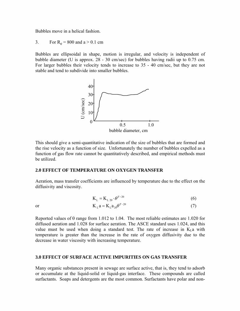
Bubbles move in a helical fashion. 3. For Re = 800 and a > 0.1 cm Bubbles are ellipsoidal in shape, motion is irregular, and velocity is independent of bubble diameter (U is approx. 28 - 30 cm/sec) for bubbles having radii up to 0.75 cm. For larger bubbles their velocity tends to increase to 35 - 40 cm/sec, but they are not stable and tend to subdivide into smaller bubbles.

0

10

30

20

40

0.5 1.0

U (c

m/s

ec)

bubble diameter, cm This should give a semi-quantitative indication of the size of bubbles that are formed and the rise velocity as a function of size. Unfortunately the number of bubbles expelled as a function of gas flow rate cannot be quantitatively described, and empirical methods must be utilized. 2.0 EFFECT OF TEMPERATURE ON OXYGEN TRANSFER Aeration, mass transfer coefficients are influenced by temperature due to the effect on the diffusivity and viscosity. 20

L L 20K K −= ⋅ Tθ (6) or 20

L L 20K a K a −= Tθ (7) Reported values of θ range from 1.012 to 1.04. The most reliable estimates are 1.020 for diffused aeration and 1.028 for surface aeration. The ASCE standard uses 1.024, and this value must be used when doing a standard test. The rate of increase in KLa with temperature is greater than the increase in the rate of oxygen diffusivity due to the decrease in water viscosity with increasing temperature. 3.0 EFFECT OF SURFACE ACTIVE IMPURITIES ON GAS TRANSFER Many organic substances present in sewage are surface active, that is, they tend to adsorb or accumulate at the liquid-solid or liquid-gas interface. These compounds are called surfactants. Soaps and detergents are the most common. Surfactants have polar and non-

polar parts of the molecule. The simplest has a polar end, often charged, and a non polar end, such as a hydrocarbon. The most common surfactant is soap, which was originally manufactured by mixing animal fat and lye (sodium hydroxide). The result is a surfactant with a negatively charged end (the sodium is released to solution as the balancing cation). Hydrogen bonding among water molecules will gradually force the surfactant’s non polar end to the surface. This happens because the polar ends of the water molecules attract each other, and squeeze the surfactant out of the way. The result is the surfactant at the interface (e.g., the air bubble surrounded by water) with the polar or charge end in the water and the non polar end protruding into the bubble. The net effect is to reduce oxygen transfer in the area around the bubble by reducing molecular diffusion of oxygen. The time required for adsorption varies with the surfactant type. Small surfactants such as acetic acid adsorb quickly. The time to reach equilibrium depends upon many different properties, but is inversely proportional the molecular weight of the surfactant. The excess surface concentration can be calculated. For a small concentration, C, in the bulk phase the surface excess can be calculated as follows:

C dRT dC

σΓ = − (8)

where R = universal gas constant T = absolute temperature Γ = surface excess (moles/cm3) C = concentration of solute σ = surface tension Basically there are four effects of surface active agents (SAA) on gas transfer: 1. The adsorbed film, which may partially or totally cover the water surface and thus

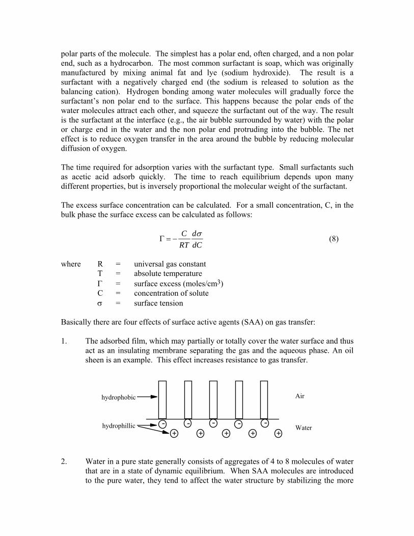
act as an insulating membrane separating the gas and the aqueous phase. An oil sheen is an example. This effect increases resistance to gas transfer.

- - - - -+ + + + +

hydrophobic

hydrophillic

Air

Water

2. Water in a pure state generally consists of aggregates of 4 to 8 molecules of water

that are in a state of dynamic equilibrium. When SAA molecules are introduced to the pure water, they tend to affect the water structure by stabilizing the more

ordered arrangements. The SAA molecules anchored to the water surface with their hydrophilic ends will acting like magnet heads that immobilize several layers of crystalline water structures and attract a blanket of counter ions. This surface hydration layer, may extend several thousand angstroms into the aqueous phase, which eliminates random surface motion (i.e., encourages surface stagnation).

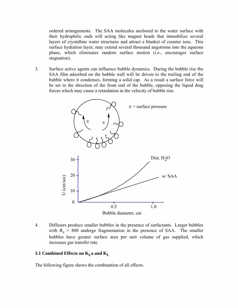
3. Surface active agents can influence bubble dynamics. During the bubble rise the

SAA film adsorbed on the bubble wall will be driven to the trailing end of the bubble where it condenses, forming a solid cap. As a result a surface force will be set in the direction of the front end of the bubble, opposing the liquid drag forces which may cause a retardation in the velocity of bubble rise.

π π

π = surface pressure

30

20

10

0 0.5 1.0

Dist. H2O

w/ SAA

Bubble diameter, cm

U (c

m/s

ec)

4. Diffusers produce smaller bubbles in the presence of surfactants. Larger bubbles

with Re > 800 undergo fragmentation in the presence of SAA. The smaller bubbles have greater surface area per unit volume of gas supplied, which increases gas transfer rate.

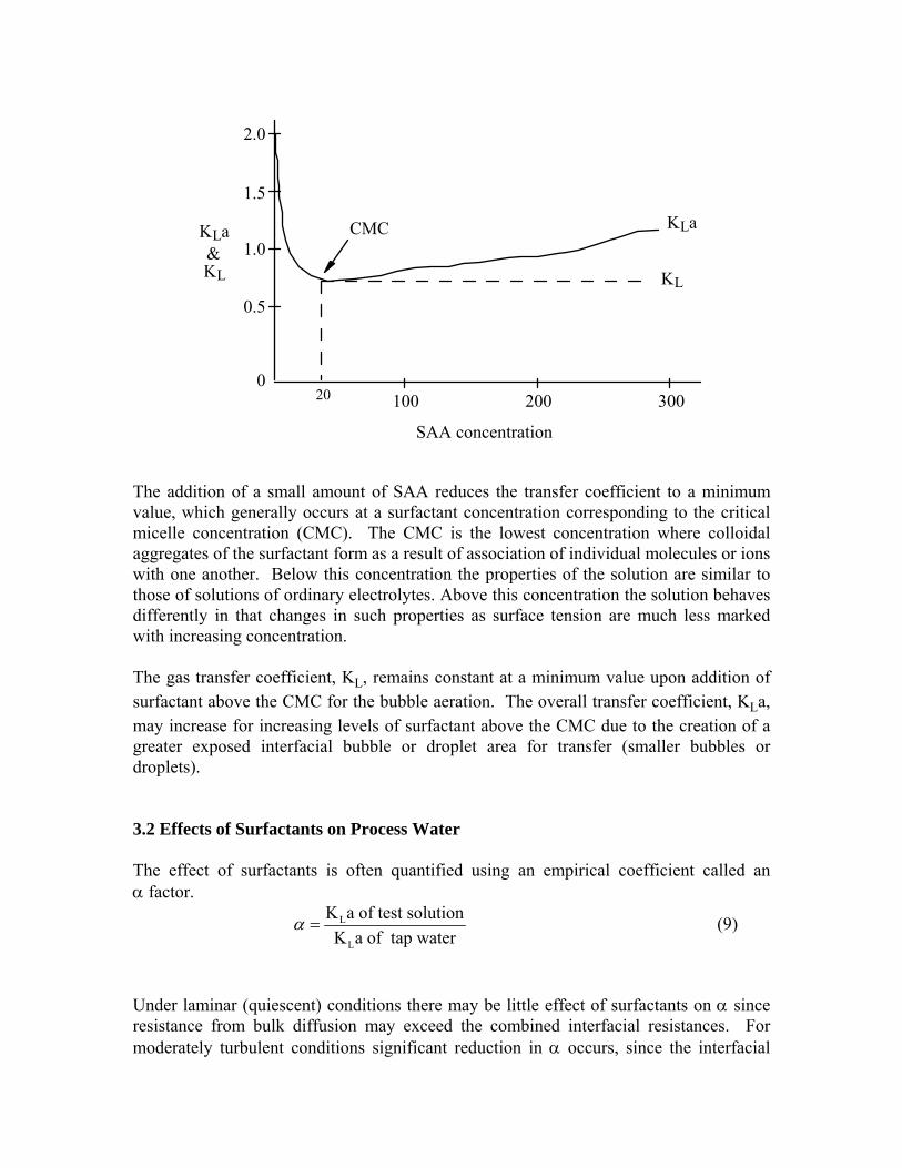
3.1 Combined Effects on KLa and KL The following figure shows the combination of all effects.

100 200 30020

0.5

1.0

1.5

2.0

0

KLa & KL

CMC

KL

KLa

SAA concentration

The addition of a small amount of SAA reduces the transfer coefficient to a minimum value, which generally occurs at a surfactant concentration corresponding to the critical micelle concentration (CMC). The CMC is the lowest concentration where colloidal aggregates of the surfactant form as a result of association of individual molecules or ions with one another. Below this concentration the properties of the solution are similar to those of solutions of ordinary electrolytes. Above this concentration the solution behaves differently in that changes in such properties as surface tension are much less marked with increasing concentration. The gas transfer coefficient, KL, remains constant at a minimum value upon addition of surfactant above the CMC for the bubble aeration. The overall transfer coefficient, KLa, may increase for increasing levels of surfactant above the CMC due to the creation of a greater exposed interfacial bubble or droplet area for transfer (smaller bubbles or droplets). 3.2 Effects of Surfactants on Process Water The effect of surfactants is often quantified using an empirical coefficient called an α factor.

L

L

K a of test solutionK a of tap water

=α (9)

Under laminar (quiescent) conditions there may be little effect of surfactants on α since resistance from bulk diffusion may exceed the combined interfacial resistances. For moderately turbulent conditions significant reduction in α occurs, since the interfacial

resistance to molecular diffusion of the adsorbed surfactant molecules controls gas transfer rate. At high degrees of turbulence the value of α may increase due to the high surface renewal rates. The high renewal prevents adsorption equilibrium at the interface; the surfactants do not have time to accumulate on the interface, because the interface is replaced or swept from the system too quickly. Values of α greater than unity may result from very high turbulence due to an increased interfacial surface area; the reduction in diffusion rate is more than compensated by the increase in interfacial surface area due to the smaller bubbles. Such conditions are rarely observed in full scale tests or treatment plants, but are easy to produce in small, lab-scale reactors. 3.3 Correlation of Bubble Aeration Data Eckenfelder (1959) showed that for any aeration depth, oxygen transfer characteristics can be correlated according to the dimensionless Sherwood, Reynolds and Schmidt numbers, as follows:

L B BK d d U ν= fD ν D

⎛ ⎞⎛ ⎞⎜ ⎟⎜ ⎟⎝ ⎠⎝ ⎠

(10)

where U = bubble velocity ν = kinematic viscosity

K LdB

D = Sherwood number (Sh)

Bd Uν

= Reynolds number (Re)

νD

= Schmidt number (Sc)

For greater aeration depths Eckenfelder applied an exponential depth factor to compensate for the end effects (formation and bursting of bubble).

( )( )1 21 3L Be c

K d H f R SD

= (11)

End effects may also be corrected for by correlating the coefficient, F, against depth. When evaluating the performance of commercial aeration equipment, one generally considers the volumetric mass transfer coefficient, KLa.

2sB

2 BB

G# bubbles area Area per minute= = ×πd =πmin bubble dd6

⎛ ⎞⎛ ⎞⎜ ⎟⎜ ⎟ ⎛ ⎞⎝ ⎠⎝ ⎠

⎜ ⎟⎝ ⎠

s6G (12)

Contact time of bubble in tank tank depth HU U

= =

Total surface area in tank of any time is therefore:

s

B

6G Hd U

= (13)

and ratio (A/V) is : s

s

6G Hd UV

(14)

Solving equation (11) for KL and multiplying by (A/V) one obtains

1 2 2 3

sL

B

H G6DK a fD d V

⎛ ⎞ν⎛ ⎞⎛ ⎞= ⎜⎜ ⎟⎜ ⎟ ⎜ν⎝ ⎠⎝ ⎠ ⎝ ⎠⎟⎟

(15)

where F6Dν

⎛ ⎝

⎞ ⎠

νD

⎛ ⎝

⎞ ⎠

1 2= constant for any gas at a particular temperature = F’

2 3

sL

B

H GK a f 'd V

⎛ ⎞= ⎜⎜

⎝ ⎠⎟⎟

(16)

Overall dB ~ Gsn

(1 n) 2 3L s

f "K a G HV

−⎛ ⎞= ⎜ ⎟⎝ ⎠

(17)

The exponent of H has been noted to vary between 0.65 and 0.99 for different types of diffusers. Equation (17) can then be rearranged (1 n) 2 3

L sK a CG H−= (18)

where f "CV

⎛ ⎞= ⎜ ⎟⎝ ⎠

One could expect reducing the tank width for the same air flow rate per unit increases the oxygen transfer efficiency while the interfacial area remains essentially constant, e.g., increases KL & KLa and therefore width must be incorporated into the model. One can then develop a transfer equation

( )m

(1-n) (T-20)s Sp

HN=CG C -C 1.024 αW

β (19)

where W = tank width, ft Gs = air flow, SCFM/aeration unit H = liquid depth, ft βCS = saturated O2 concentration in waste N = transfer rate, lbs O2/hr/aeration unit

Pressure G 144HP33,000 e

= (power required for the blower) (20)

Where HP is the horsepower required for the blower, Pressure is the total discharge pressure in PSI, G is the gas flow in SCFM and e is the efficiency as a fraction. 3.4 Turbine Aerators In turbine aeration, air is discharged from a sparge ring beneath a rotating impeller. The action of the impeller forces flow downward, shearing the bubbles (making them smaller with higher surface renewal). Air flow, diameter and speed all influence KLa. From equation (18) one can develop ym n

s stN CR G d (C C)= − (21) and HP = Cdt

nRm Power drawn by turbine (22) where, R = impeller peripheral speed (ft/sec) dt = impeller diameter (ft) n,m = empirical coefficients based upon impeller geometry. Optimal conditions for most turbines exist when the power required to compress the air that is discharged below the turbine impeller equals the impeller’s power. 3.5 Surface Aerators Oxygen is transferred to droplets from the atmosphere and from the bubbles to the bulk solution.

( )s (T-20)o

βC -CN=N α 1.024

9.07 (23)

where No = transfer rate for standard conditions, 20oC, zero DO (lbs O2/HP-hr) Cs = Saturation value of dissolved oxygen (9.07 at 20oC, in pure water) β = Ratio of oxygen saturation in process water to tap water

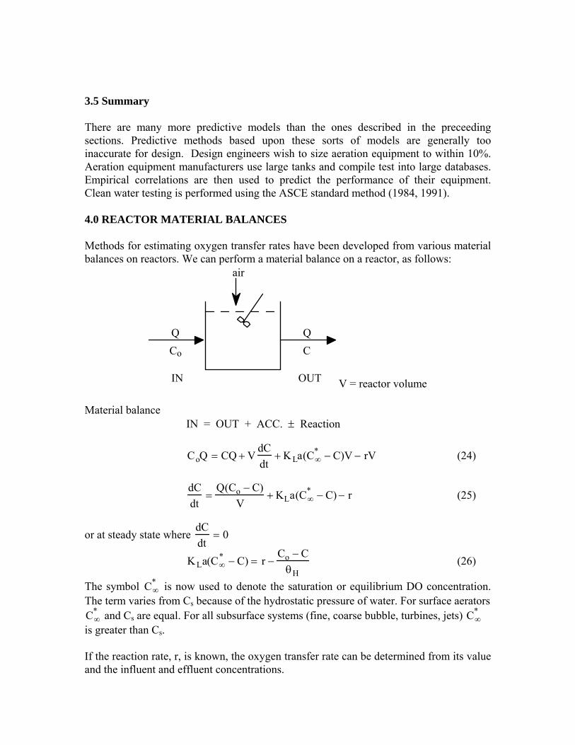
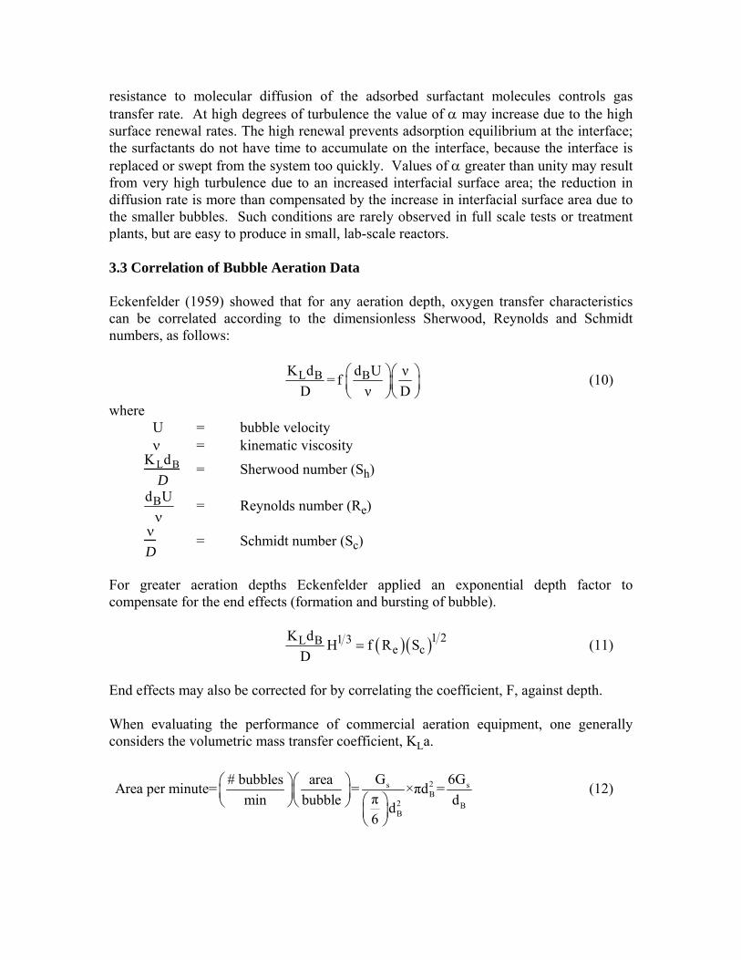
3.5 Summary There are many more predictive models than the ones described in the preceeding sections. Predictive methods based upon these sorts of models are generally too inaccurate for design. Design engineers wish to size aeration equipment to within 10%. Aeration equipment manufacturers use large tanks and compile test into large databases. Empirical correlations are then used to predict the performance of their equipment. Clean water testing is performed using the ASCE standard method (1984, 1991). 4.0 REACTOR MATERIAL BALANCES Methods for estimating oxygen transfer rates have been developed from various material balances on reactors. We can perform a material balance on a reactor, as follows:

air

QCo

QC

IN OUT V = reactor volume Material balance IN = OUT + ACC. ± Reaction

CoQ = CQ + VdCdt

+ KLa(C∞* − C)V − rV (24)

dCdt

=Q(Co − C)

V+ KLa(C∞

* − C) − r (25)

or at steady state where dCdt

= 0

KLa(C∞* − C) = r −

Co − CθH

(26)

The symbol C is now used to denote the saturation or equilibrium DO concentration. The term varies from C

∞*

s because of the hydrostatic pressure of water. For surface aerators C∞

* and Cs are equal. For all subsurface systems (fine, coarse bubble, turbines, jets) C∞*

is greater than Cs. If the reaction rate, r, is known, the oxygen transfer rate can be determined from its value and the influent and effluent concentrations.

For the special case when Q equals zero or batch conditions, equation 26 reduces to

KLa =r

C∞* − C

(27)

This is the very well known steady state batch equilibrium equation for estimating gas transfer from a measured value of r. One measures C and estimates C from other knowledge, such as temperature and pressure, or clean water data and calculates K

∞*

La. The problem with this method is estimating r. Often it is necessary to vary C (DO concentration) to measure r, and in doing so, one changes r. A biological culture’s reaction rate is independent of the DO concentration above some minimum value, and this might be 0.5 to 2.0 mg/L for low-rate, non-nitrifying systems. For high rate or nitrifying systems, the rate may vary, even up to 4.0 mg/L. Therefore, great care must be exercised when using equation 27 to estimate process water transfer rate. For non-steady state, batch

dCdt

= KLa(C∞* − C) (28)

after integration C = C∞

* − (C∞* − Ci )e

−KLat (29) This equation is used for the ASCE Standard Method. One can add continuity terms to equation 28 (no longer batch) and integrate to obtain continuous flow design equations. NON-STEADY STATE REAERATION TEST This test is the basis for clean water testing which is used for most performance testing of aeration equipment. The test is performed and the data are analyzed based upon one of equation 29. To perform the test, one usually supplies a deoygenating chemical to remove the oxygen. Aeration is provided and the rates of transfer are calculated from the rate at which the water is reaerated. In other terms, one removes the dissolved oxygen from the reactor and then restores it, while measuring the rate. The graph below shows the DO concentration during a test. The sulfite is quickly added and the DO plunges quite rapidly to zero or near zero. After some period, the DO returns and the concentration gradually increases to the equilibrium value. The sulfite reaction is catalyzed to increase its speed, and any practical aeration system, no DO is observed in the presence of sulfite. Once the sulfite is completely reacted, DO is observed. To perform a nonsteady-state reaeration test, one adds sodium sulfite to deaerate or strip the water of DO, as follows: 1/2 O2 + Na2SO3 → Na2SO4 The reaction is very fast and is catalyzed by cobalt ions. Cobalt is usually added as cobalt-chloride. The reaction is so rapid that measurable DO and sulfite are present at the

same time. Usually only 0.05 mg/L of cobalt (as Co) is required. Above 0.5 mg/L interferences of cobalt and the Winkler DO measurement procedure are sometimes observed.

t

add Na2SO3

DO

C∞*

Sulfite is usually added by first dissolving the sulfite in water and then pumping the water into the reactor. This avoids clumps of sulfite that dissolve too slowly. A saturated sulfite solution contains 2.23 lb/gal at 20oC and 3.00 lb/gal at 30oC. Add 7.88 mg/L sulfite per 1 mg/L DO plus some excess to insure that all the DO is removed. For low rate aeration systems, usually only 25% extra is added. For very large systems, as much as 100% excess is added. There needs to be a period of near-zero DO, as shown above to obtain reliable results. The test results can be analyzed using three different forms of the previously developed mass transfer equation. The forms are log deficit (from equation 29), differential (from equation 28) and exponential (also from equation 29). They are described as follows: Log Deficit

C∞

* − CC∞

* − Ci= e−KLat (30)

lnC∞

* − CC∞

* − Ci= −KLat (31)

or ln C∞* − C = ln C∞

* − Ci − KLat (32) We can fit data with a straight line by plotting the left side of equation 32 versus time. The result is a straight line with slope -KLa. . It is linear in the parameter KLa, and nonlinear in C .You must know the value of C∞

*∞* from other methods, often called a

priori methods. Differential form

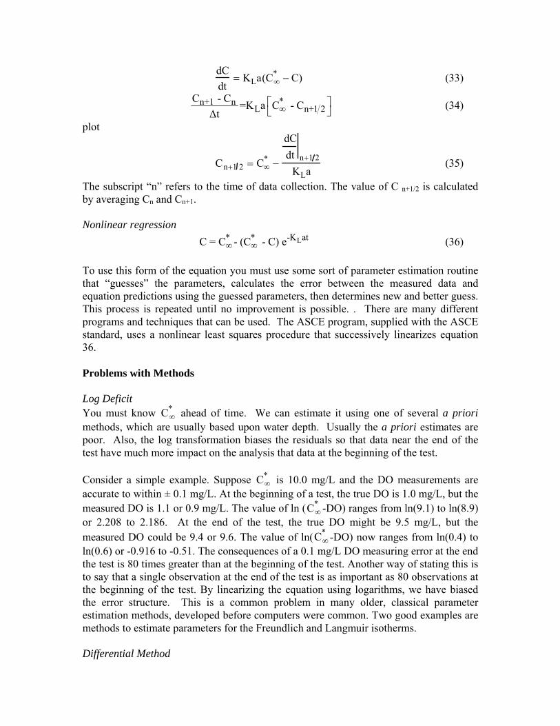
dCdt

= KLa(C∞* − C) (33)

*n+1 nL n+

C - C =K a C - CΔt ∞ 1 2⎡ ⎤

⎣ ⎦ (34)

plot

Cn+1 2 = C∞* −

dCdt n+1 2

KLa (35)

The subscript “n” refers to the time of data collection. The value of C n+1/2 is calculated by averaging Cn and Cn+1. Nonlinear regression (36) L-K at* *C = C - (C - C) e∞ ∞ To use this form of the equation you must use some sort of parameter estimation routine that “guesses” the parameters, calculates the error between the measured data and equation predictions using the guessed parameters, then determines new and better guess. This process is repeated until no improvement is possible. . There are many different programs and techniques that can be used. The ASCE program, supplied with the ASCE standard, uses a nonlinear least squares procedure that successively linearizes equation 36. Problems with Methods Log Deficit You must know C ahead of time. We can estimate it using one of several a priori methods, which are usually based upon water depth. Usually the a priori estimates are poor. Also, the log transformation biases the residuals so that data near the end of the test have much more impact on the analysis that data at the beginning of the test.

∞*

Consider a simple example. Suppose C∞

* is 10.0 mg/L and the DO measurements are accurate to within ± 0.1 mg/L. At the beginning of a test, the true DO is 1.0 mg/L, but the measured DO is 1.1 or 0.9 mg/L. The value of ln (C∞

* -DO) ranges from ln(9.1) to ln(8.9) or 2.208 to 2.186. At the end of the test, the true DO might be 9.5 mg/L, but the measured DO could be 9.4 or 9.6. The value of ln(C∞

* -DO) now ranges from ln(0.4) to ln(0.6) or -0.916 to -0.51. The consequences of a 0.1 mg/L DO measuring error at the end the test is 80 times greater than at the beginning of the test. Another way of stating this is to say that a single observation at the end of the test is as important as 80 observations at the beginning of the test. By linearizing the equation using logarithms, we have biased the error structure. This is a common problem in many older, classical parameter estimation methods, developed before computers were common. Two good examples are methods to estimate parameters for the Freundlich and Langmuir isotherms. Differential Method

The differential method magnifies the noise in the data. For example, suppose the DO has noise as follows: C = DO + Asin2πωt (37) when 2πω ≡ power line frequency (60Hz) = 2 (3.14) x 60 ≅ 360

dCdt

=dDO

dt+ 360Acos(2πωt) (38)

The noise is multiplied 360 fold! Residuals are greater at the beginning of the test, which biases the early data points. This is the opposite sort of bias from the log-deficit method. Exponential This method is by far the best, but requires a computer or programmable calculator. It does not bias the residuals, but they are usually greatest at the beginning of the test. It is also harder for some people to understand. The analysis provides estimates of KLa, Ci and C∞

* . The ASCE standard provides a computer code and example program using Visual Basic and Excel. Some useful information about testing. Definitions, from the ASCE standard.

Standard Conditions. 20oC 1 ATM pressure 760 mm Hg 100% RH 0 TDS Tap water < 500 ~ 200 mg/L 0 = mg/L DO

SOTR = Standard Oxygen Transfer Rate (mass/time = lb/hr, or kg/hr) SOTE = Standard Oxygen Transfer Efficiency (%) mass transferred and applicable only

to subsurface aerators. SAE = Standard Aeration Efficiency (lb O2/hp-hr or kg O2/kW-hr) (39) SOTR = KLa20C∞20

* V SAE = SOTR / Power Input (40) SOTE = SOTR / Mass Gas Flow Rate (41)

=SOTR

1.034Qs (42)

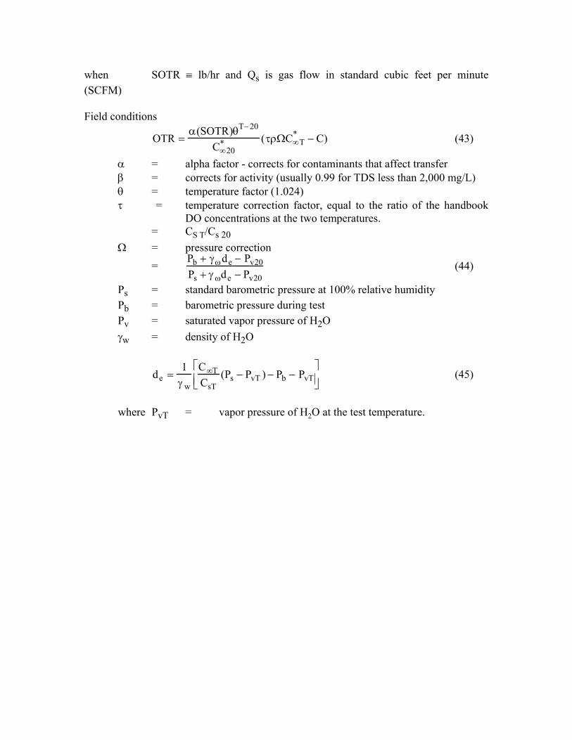
when SOTR ≡ lb/hr and Qs is gas flow in standard cubic feet per minute (SCFM) Field conditions

OTR =α(SOTR)θT−20

C∞20* (τρΩC∞T

* − C) (43)

α = alpha factor - corrects for contaminants that affect transfer β = corrects for activity (usually 0.99 for TDS less than 2,000 mg/L) θ = temperature factor (1.024)

τ = temperature correction factor, equal to the ratio of the handbook DO concentrations at the two temperatures.

= CS T/Cs 20 Ω = pressure correction

= Pb + γωde − Pv20Ps + γ ωde − Pv20

(44)

Ps = standard barometric pressure at 100% relative humidity Pb = barometric pressure during test Pv = saturated vapor pressure of H2O γw = density of H2O

de =1

γ w

C∞TCsT

(Ps − PvT ) − Pb − PvT⎡

⎣ ⎢ ⎤

⎦ ⎥ (45)

where PvT = vapor pressure of H2O at the test temperature.

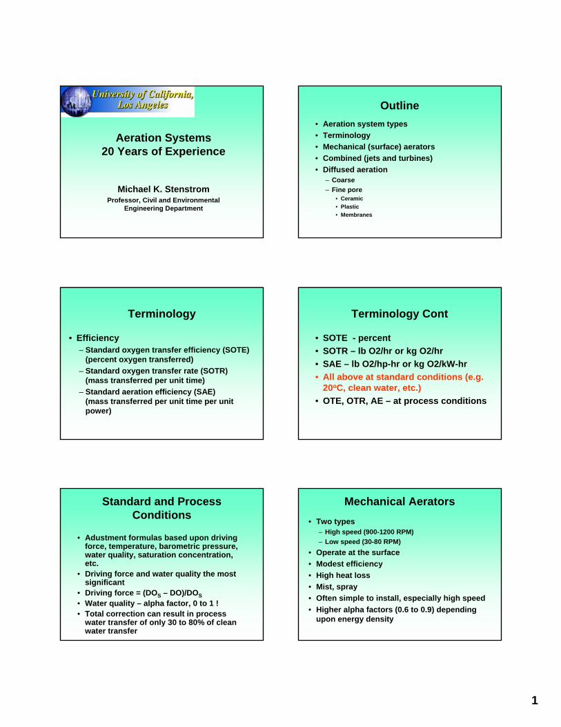
1

Aeration Systems20 Years of Experience

Michael K. StenstromProfessor, Civil and Environmental

Engineering Department

Outline• Aeration system types• Terminology• Mechanical (surface) aerators• Combined (jets and turbines)• Diffused aeration

– Coarse– Fine pore

• Ceramic• Plastic• Membranes

Terminology

• Efficiency– Standard oxygen transfer efficiency (SOTE)

(percent oxygen transferred)– Standard oxygen transfer rate (SOTR)

(mass transferred per unit time)– Standard aeration efficiency (SAE)

(mass transferred per unit time per unit power)

Terminology Cont

• SOTE - percent• SOTR – lb O2/hr or kg O2/hr• SAE – lb O2/hp-hr or kg O2/kW-hr• All above at standard conditions (e.g.

20oC, clean water, etc.)• OTE, OTR, AE – at process conditions

Standard and Process Conditions

• Adustment formulas based upon driving force, temperature, barometric pressure, water quality, saturation concentration, etc.

• Driving force and water quality the most significant

• Driving force = (DOS – DO)/DOS• Water quality – alpha factor, 0 to 1 !• Total correction can result in process

water transfer of only 30 to 80% of clean water transfer

Mechanical Aerators• Two types

– High speed (900-1200 RPM)– Low speed (30-80 RPM)

• Operate at the surface• Modest efficiency• High heat loss• Mist, spray• Often simple to install, especially high speed• Higher alpha factors (0.6 to 0.9) depending

upon energy density

2

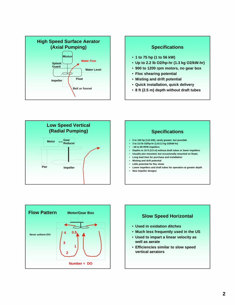
High Speed Surface Aerator(Axial Pumping)

FloatImpeller

Water Level

SplashGuard

Water Flow

Specifications

• 1 to 75 hp (1 to 56 kW)• Up to 2.2 lb O2/hp-hr (1.3 kg O2/kW-hr)• 900 to 1200 rpm motors, no gear box• Floc shearing potential• Misting and drift potential• Quick installation, quick delivery• 8 ft (2.5 m) depth without draft tubes

Low Speed Vertical(Radial Pumping)

Motor GearReducer

ImpellerPier

Specifications• 5 to 150 hp (112 kW), rarely greater, but possible• 3 to 3.5 lb O2/hp-hr (1.8-2.2 kg O2/kW-hr)• ~40 to 80 RPM impellers• Depths to 15 ft (3.5 m) without draft tubes or lower impellers• Usually pier mounted, but occasionally mounted on floats• Long lead time for purchase and installation• Misting and drift potential• Little potential for floc shear• Lower impellers and draft tubes for operation at greater depth• New impeller designs

Flow Pattern Motor/Gear Box

Number = DO

4

3

2

1

0.5Never uniform DO!

Slow Speed Horizontal

• Used in oxidation ditches• Much less frequently used in the US• Used to impart a linear velocity as

well as aerate• Efficiencies similar to slow speed

vertical aerators

3

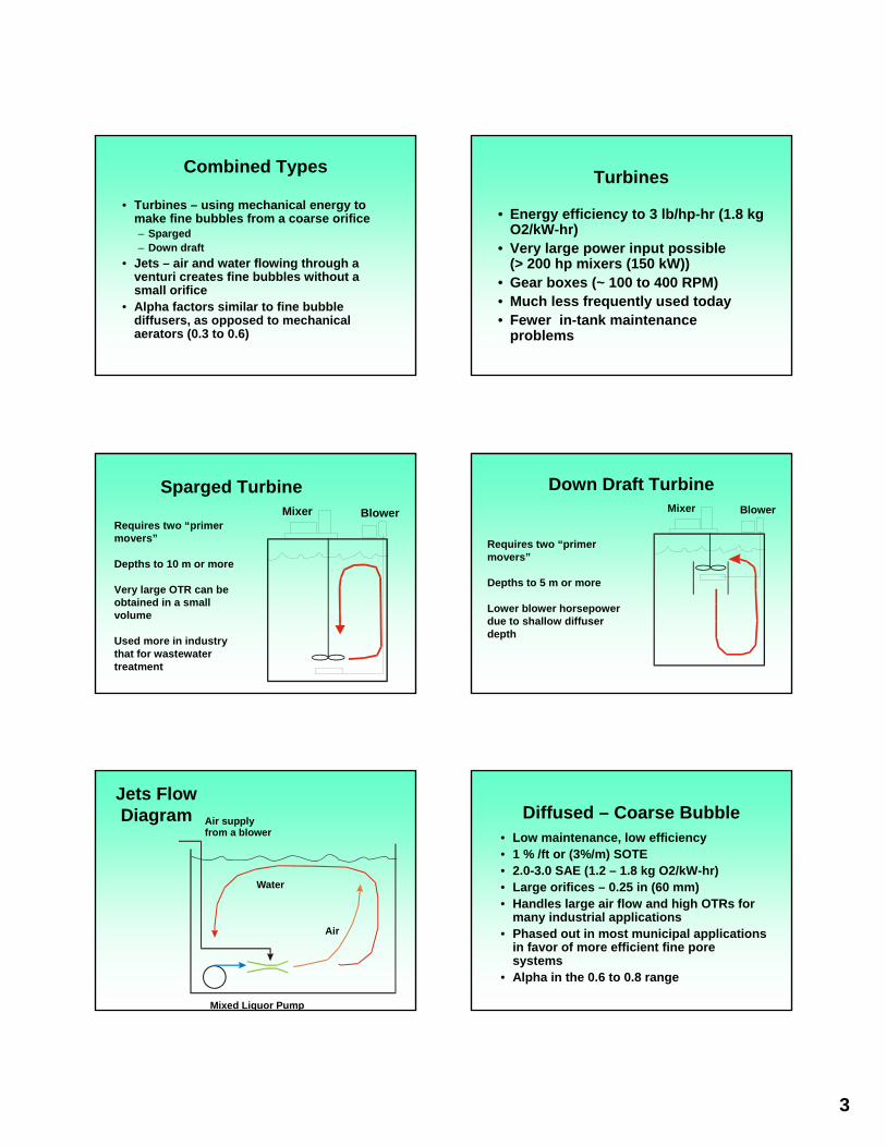
Combined Types

• Turbines – using mechanical energy to make fine bubbles from a coarse orifice– Sparged – Down draft

• Jets – air and water flowing through a venturi creates fine bubbles without a small orifice

• Alpha factors similar to fine bubble diffusers, as opposed to mechanical aerators (0.3 to 0.6)

Turbines

• Energy efficiency to 3 lb/hp-hr (1.8 kg O2/kW-hr)

• Very large power input possible (> 200 hp mixers (150 kW))

• Gear boxes (~ 100 to 400 RPM)• Much less frequently used today• Fewer in-tank maintenance

problems

Sparged Turbine

Requires two “primer movers”

Depths to 10 m or more

Very large OTR can be obtained in a small volume

Used more in industry that for wastewater treatment

Mixer Blower

Down Draft Turbine

Requires two “primer movers”

Depths to 5 m or more

Lower blower horsepower due to shallow diffuser depth

Mixer Blower

Jets Flow Diagram Air supply

from a blower

Mixed Liquor Pump

Water

Air

Diffused – Coarse Bubble• Low maintenance, low efficiency • 1 % /ft or (3%/m) SOTE • 2.0-3.0 SAE (1.2 – 1.8 kg O2/kW-hr)• Large orifices – 0.25 in (60 mm)• Handles large air flow and high OTRs for

many industrial applications• Phased out in most municipal applications

in favor of more efficient fine pore systems

• Alpha in the 0.6 to 0.8 range

4

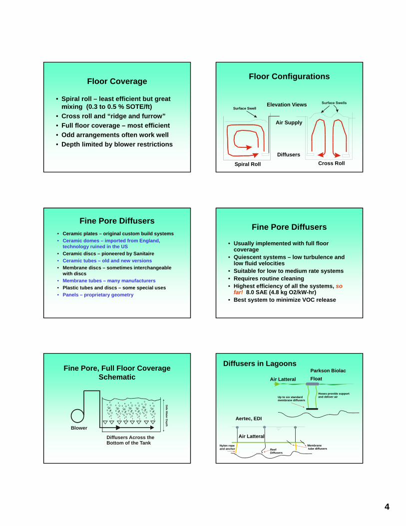
Floor Coverage

• Spiral roll – least efficient but great mixing (0.3 to 0.5 % SOTE/ft)

• Cross roll and “ridge and furrow”• Full floor coverage – most efficient• Odd arrangements often work well• Depth limited by blower restrictions

Floor Configurations

Air Supply

Diffusers

Elevation Views

Spiral Roll Cross Roll

Surface Swell

Fine Pore Diffusers• Ceramic plates – original custom build systems• Ceramic domes – imported from England,

technology ruined in the US• Ceramic discs – pioneered by Sanitaire• Ceramic tubes – old and new versions• Membrane discs – sometimes interchangeable

with discs• Membrane tubes – many manufacturers• Plastic tubes and discs – some special uses• Panels – proprietary geometry

Fine Pore Diffusers

• Usually implemented with full floor coverage

• Quiescent systems – low turbulence and low fluid velocities

• Suitable for low to medium rate systems• Requires routine cleaning• Highest efficiency of all the systems, so

far! 8.0 SAE (4.8 kg O2/kW-hr)• Best system to minimize VOC release

Fine Pore, Full Floor Coverage Schematic

Blower

Diffusers Across the Bottom of the Tank

Side Water D

epth

Diffusers in Lagoons

Air Latteral Float

Hoses provide support and deliver airUp to six standard

membrane diffusers

Parkson Biolac

Aertec, EDI

Membrane tube diffusersReef

Diffusers

Air Latteral

Nylon ropeand anchor

5

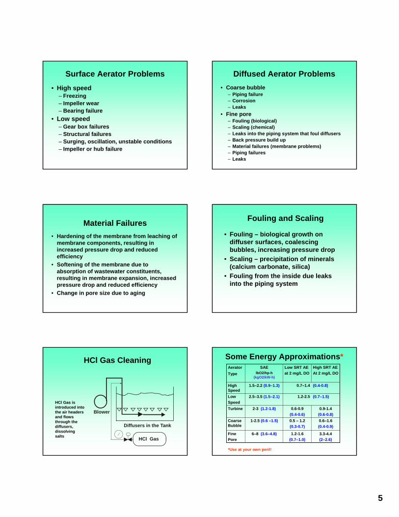
Surface Aerator Problems• High speed

– Freezing– Impeller wear– Bearing failure

• Low speed– Gear box failures– Structural failures– Surging, oscillation, unstable conditions– Impeller or hub failure

Diffused Aerator Problems• Coarse bubble

– Piping failure– Corrosion– Leaks

• Fine pore– Fouling (biological)– Scaling (chemical)– Leaks into the piping system that foul diffusers– Back pressure build up– Material failures (membrane problems)– Piping failures– Leaks

Material Failures• Hardening of the membrane from leaching of

membrane components, resulting in increased pressure drop and reduced efficiency

• Softening of the membrane due to absorption of wastewater constituents, resulting in membrane expansion, increased pressure drop and reduced efficiency

• Change in pore size due to aging

Fouling and Scaling

• Fouling – biological growth on diffuser surfaces, coalescing bubbles, increasing pressure drop

• Scaling – precipitation of minerals (calcium carbonate, silica)

• Fouling from the inside due leaks into the piping system

HCl Gas Cleaning

Blower

Diffusers in the Tank

HCl Gas

HCl Gas is introduced into the air headers and flows through the diffusers, dissolving salts

Some Energy Approximations*

3.3-4.4 (2–2.6)

1.2-1.6 (0.7–1.0)

6–8 (3.6–4.8)Fine Pore

0.6–1.6 (0.4-0.9)

0.5 – 1.2 (0.3-0.7)

1-2.5 (0.6 –1.5)Coarse Bubble

0.9-1.4 (0.6-0.8)

0.6-0.9 (0.4-0.6)

2-3 (1.2-1.8)Turbine

(0.7–1.5)1.2-2.5 2.5–3.5 (1.5–2.1)Low Speed

(0.4-0.8)0.7–1.4 1.5–2.2 (0.9–1.3)High Speed

High SRT AEAt 2 mg/L DO

Low SRT AEat 2 mg/L DO

SAElbO2/hp-h

(kgO2/kW-h)

Aerator Type

*Use at your own peril!

6

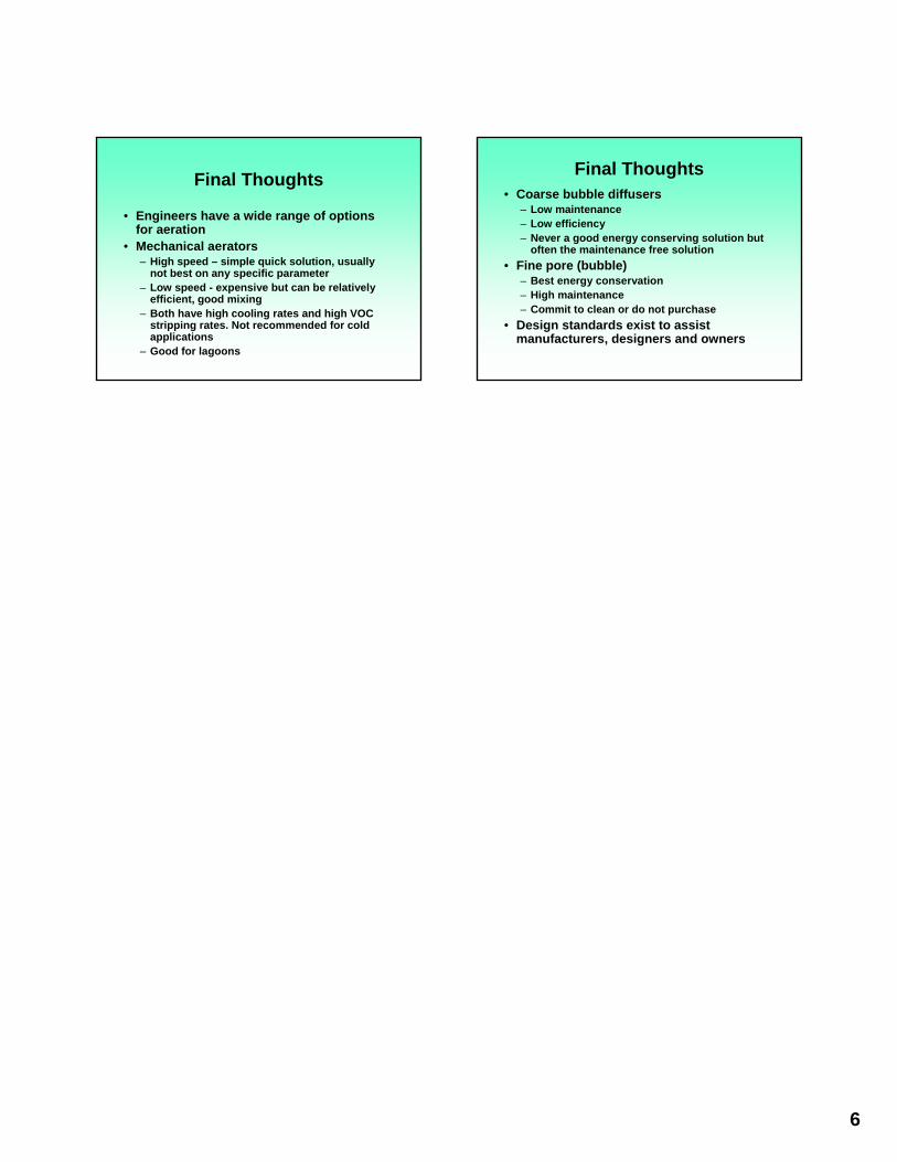
Final Thoughts

• Engineers have a wide range of options for aeration

• Mechanical aerators– High speed – simple quick solution, usually

not best on any specific parameter– Low speed - expensive but can be relatively

efficient, good mixing– Both have high cooling rates and high VOC

stripping rates. Not recommended for cold applications

– Good for lagoons

Final Thoughts• Coarse bubble diffusers

– Low maintenance– Low efficiency– Never a good energy conserving solution but

often the maintenance free solution• Fine pore (bubble)

– Best energy conservation– High maintenance– Commit to clean or do not purchase

• Design standards exist to assist manufacturers, designers and owners

1

Copy right 2000 Michael K. Stenstrom

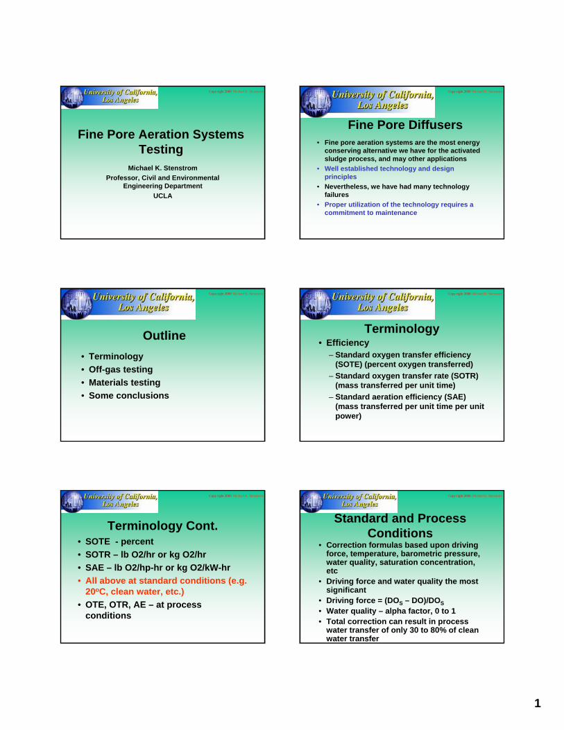
Fine Pore Aeration Systems Testing

Michael K. StenstromProfessor, Civil and Environmental

Engineering DepartmentUCLA

Copy right 2000 Michael K. Stenstrom

Fine Pore Diffusers• Fine pore aeration systems are the most energy

conserving alternative we have for the activated sludge process, and may other applications

• Well established technology and design principles

• Nevertheless, we have had many technology failures

• Proper utilization of the technology requires a commitment to maintenance

Copy right 2000 Michael K. Stenstrom

Outline• Terminology• Off-gas testing• Materials testing• Some conclusions

Copy right 2000 Michael K. Stenstrom

Terminology• Efficiency

– Standard oxygen transfer efficiency (SOTE) (percent oxygen transferred)

– Standard oxygen transfer rate (SOTR) (mass transferred per unit time)

– Standard aeration efficiency (SAE) (mass transferred per unit time per unit power)

Copy right 2000 Michael K. Stenstrom

Terminology Cont.• SOTE - percent• SOTR – lb O2/hr or kg O2/hr• SAE – lb O2/hp-hr or kg O2/kW-hr• All above at standard conditions (e.g.

20oC, clean water, etc.)• OTE, OTR, AE – at process

conditions

Copy right 2000 Michael K. Stenstrom

Standard and Process Conditions

• Correction formulas based upon driving force, temperature, barometric pressure, water quality, saturation concentration, etc

• Driving force and water quality the most significant

• Driving force = (DOS – DO)/DOS• Water quality – alpha factor, 0 to 1• Total correction can result in process

water transfer of only 30 to 80% of clean water transfer

2

Copy right 2000 Michael K. Stenstrom

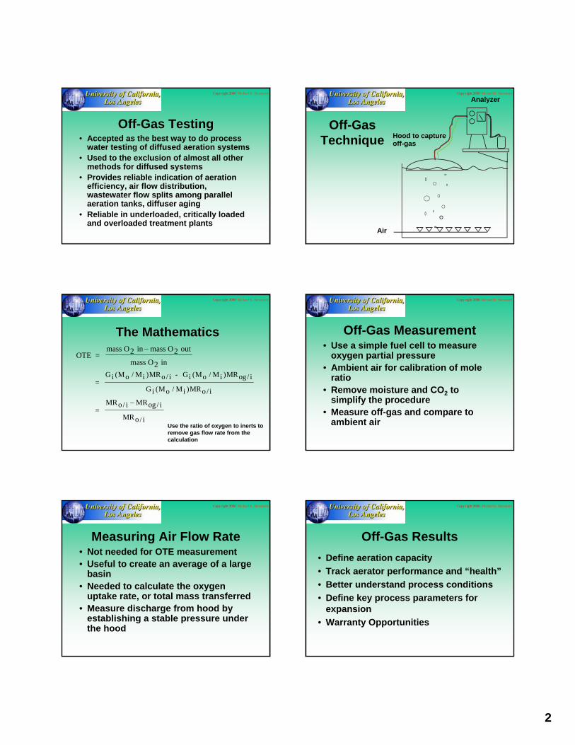
Off-Gas Testing• Accepted as the best way to do process

water testing of diffused aeration systems• Used to the exclusion of almost all other

methods for diffused systems• Provides reliable indication of aeration

efficiency, air flow distribution, wastewater flow splits among parallel aeration tanks, diffuser aging

• Reliable in underloaded, critically loaded and overloaded treatment plants

Copy right 2000 Michael K. Stenstrom

Off-Gas Technique

Air

Analyzer

Hood to capture off-gas

Copy right 2000 Michael K. Stenstrom

The MathematicsOTE

mass O mass O

mass O= 2 in out

2 in

− 2

= Gi - Gi

Gi

( / ) / ( / ) /

( / ) /

Mo Mi MRo i Mo Mi MRog i

Mo Mi MRo i

= MRo i MRog i

MRo i

/ /

/

−

Use the ratio of oxygen to inerts to remove gas flow rate from the calculation

Copy right 2000 Michael K. Stenstrom

Off-Gas Measurement• Use a simple fuel cell to measure

oxygen partial pressure• Ambient air for calibration of mole

ratio• Remove moisture and CO2 to

simplify the procedure • Measure off-gas and compare to

ambient air

Copy right 2000 Michael K. Stenstrom

Measuring Air Flow Rate• Not needed for OTE measurement• Useful to create an average of a large

basin• Needed to calculate the oxygen

uptake rate, or total mass transferred• Measure discharge from hood by

establishing a stable pressure under the hood

Copy right 2000 Michael K. Stenstrom

Off-Gas Results• Define aeration capacity• Track aerator performance and “health”• Better understand process conditions• Define key process parameters for

expansion• Warranty Opportunities

3

Copy right 2000 Michael K. Stenstrom

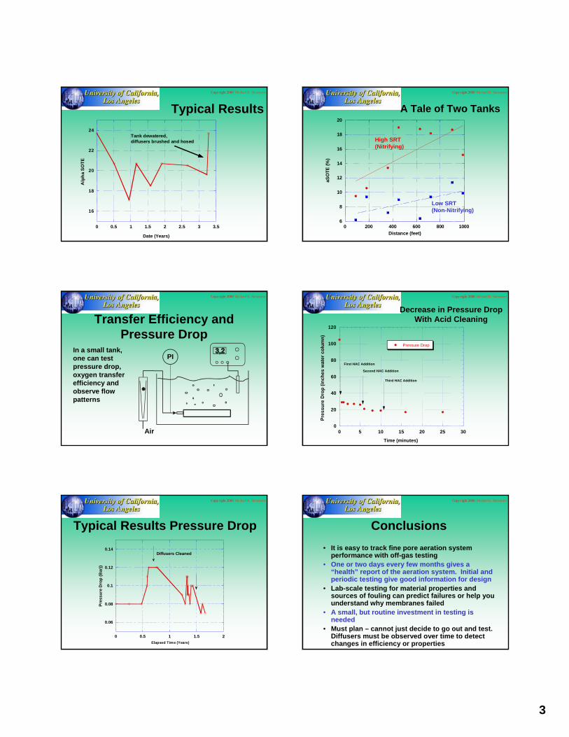
16

18

20

22

24

0 0.5 1 1.5 2 2.5 3 3.5

Alp

ha S

OTE

Date (Years)

Tank dewatered, diffusers brushed and hosed

Typical ResultsCopy right 2000 Michael K. Stenstrom

6

8

10

12

14

16

18

20

0 200 400 600 800 1000

aSO

TE (%

)

Distance (feet)

A Tale of Two Tanks

High SRT(Nitrifying)

Low SRT(Non-Nitrifying)

Copy right 2000 Michael K. Stenstrom

Transfer Efficiency and Pressure Drop

Air

PIIn a small tank, one can test pressure drop, oxygen transfer efficiency and observe flow patterns

Copy right 2000 Michael K. Stenstrom

0

20

40

60

80

100

120

0 5 10 15 20 25 30

Pressure Drop

Pres

sure

Dro

p (in

ches

wat

er c

olum

n)

Time (minutes)

First HAC Addition

Second HAC Addition

Third HAC Addition

Decrease in Pressure Drop With Acid Cleaning

Copy right 2000 Michael K. Stenstrom

0.06

0.08

0.1

0.12

0.14

0 0.5 1 1.5 2

Pres

sure

Dro

p (B

ar))

Elapsed Time (Years)

Diffusers Cleaned

Typical Results Pressure Drop

Copy right 2000 Michael K. Stenstrom

Conclusions• It is easy to track fine pore aeration system

performance with off-gas testing• One or two days every few months gives a

“health” report of the aeration system. Initial and periodic testing give good information for design

• Lab-scale testing for material properties and sources of fouling can predict failures or help you understand why membranes failed

• A small, but routine investment in testing is needed

• Must plan – cannot just decide to go out and test. Diffusers must be observed over time to detect changes in efficiency or properties