Modeling Discrete Combinatorial Systems asAlphabetic Bipartite Networks (α-BiNs): Theory and Applications

Monojit ChoudhuryMicrosoft Research India,196/36 2nd Main Sadashivnagar, Bangalore 560080, India.

Niloy GangulyDepartment of Computer Science and Engineering,

Indian Institute of Technology Kharagpur, Kharagpur 721302, India.

Abyayananda Maiti and Animesh MukherjeeDepartment of Computer Science and Engineering,

Indian Institute of Technology Kharagpur, 721302 Kharagpur, India.

Lutz Brusch and Andreas DeutschZIH, TU Dresden, Zellescher Weg 12, 01069 Dresden, Germany.

Fernando Peruani∗

CEA-Service de Physique de l’Etat Condense, Centre d’Etudes de Saclay, 91191 Gif-sur-Yvette, France,Institut des Systemes Complexes de Paris Ile-de-France, 57/59, rue Lhomond, F-75005 Paris, France.

(Dated: April 13, 2009)

Life and language are discrete combinatorial systems (DCSs) in which the basic building blocksare finite sets of elementary units: nucleotides or codons in a DNA sequence and letters or wordsin a language. Different combinations of these finite units give rise to potentially infinite numbersof genes or sentences. This type of DCS can be represented as an Alphabetic Bipartite Network(α-BiN) where there are two kinds of nodes, one type represents the elementary units while theother type represents their combinations. There is an edge between a node corresponding to anelementary unit u and a node corresponding to a particular combination v if u is present in v.Naturally, the partition consisting of the nodes representing elementary units is fixed, while theother partition is allowed to grow unboundedly. Here, we extend recent analytical findings forα-BiNs derived in [Europhys. Lett. 79, 28001 (2007)] and empirically investigate two real worldsystems: the codon-gene network and the phoneme-language network. The evolution equationsfor α-BiNs under different growth rules are derived, and the corresponding degree distributionscomputed. It is shown that asymptotically the degree distribution of α-BiNs can be described as afamily of beta distributions. The one-mode projections of the theoretical as well as the real worldα-BiNs are also studied. We propose a comparison of the real world degree distributions and ourtheoretical predictions as a means for inferring the mechanisms underlying the growth of real worldsystems.

I. INTRODUCTION

Two of the greatest wonders of evolution on earth,life and language, are discrete combinatorial systems(DCSs) [1]. The basic building blocks of DCSs are finitesets of elementary units, such as the letters in languageand nucleotides (or codons) in DNA. Different combina-tions of these finite elementary units give rise to a po-tentially infinite number of words or genes. Here, wepropose a special class of complex networks as a modelof DCSs. We shall refer to them as Alphabetic BipartiteNetworks (α-BiNs) in order to signify the fact that theset of basic units, in both human and genetic languages,can be considered as an Alphabet.

The α-BiNs are a subclass of bipartite networks where

∗Corresponding author: peruani@pks.mpg.de

there are two disjoint partitions of nodes. An edge, ina bipartite network, links nodes that appear in two dif-ferent partitions, but never those belonging to the samepartition. In most of the bipartite networks studied inthe past both the partitions grow with time. Typicalexamples of this type of networks include collaborationnetworks such as the movie-actor [2–6], article-author [7–9], and board-director [10, 11] networks. In the article-author network, for instance, the articles and authors arethe elements of the two partitions also known as the tiesand actors respectively. An edge between an author aand an article m indicates that a has co-authored m. Theauthors a and a′ are collaborators if both have coauthoredthe same article, i.e., if both are connected to the samenode m. The concept of collaboration can be extendedto represent, through bipartite networks, several diversephenomena such as the city-people network [12], in whichan edge between a person and a city indicates that theperson has visited that particular city, the signal-objectnetwork in linguistics [13], where an edge between an ob-

2

ject j and a signal i represents that a possible meaningof the i sign is the object j, the bank-company [16] ordonor-acceptor network that accounts for injection andmerging of magnetic field lines [17].

Several models have been proposed to synthesize thestructure of these bipartite networks, i.e., when boththe partitions grow unboundedly over time [2–5, 15]. Ithas been found that for such growth models, when eachincoming tie node preferentially attaches itself to theactor nodes, the emergent degree distribution of the actornodes follows a power-law [2]. This result is reminiscentof unipartite networks where preferential attachment re-sults in power-law degree distributions [18].

Although there have been some works on non-growingbipartite networks [19, 20] those like α-BiNs where oneof the partitions remains fixed over time have receivedcomparatively much less attention. Since the set of ba-sic units in DCSs is always finite and constant, α-BiNshave one of its partitions fixed, the one that representsthe basic units (e.g. letters, codons). In contrast, theother partition, that represents the unique discrete com-binations of basic unit (e.g., words, genes), can grow un-boundedly over time. Notice that the order in which thebasic units are strung to form the discrete combinationis an important and indispensable aspect of the system,which can be modeled within the framework of α-BiNs byallowing ordering of the edges. Nevertheless, the scope ofthe present work is limited to the analysis of unorderedcombinations. Here we assume a word to be a bag of let-ters and a gene a collection of codons. Fig. 1 illustratesthe concepts through the example of genes and codons.

As far as we know, the first empirical evidence of thenon-scale free character of the degree distribution of α-BiNs has been reported in [21], while the first systematicand analytical study of such bipartite networks has beenpresented in [22]. The growth model for α-BiNs, pro-posed in [22], is based on a preferential attachment cou-pled with a tunable randomness component. Accordingto this model, there is a free parameter γ which controlsthe relative weight of preferential to random attachment,thereby, regulating the randomness present in the con-nections of the network. For sequential attachment, i.e.,when the edges are incorporated one by one, the exactexpression for the emergent degree distribution has beenderived. Nevertheless, for parallel attachment, i.e., whenmultiple edges are incorporated in one time step, onlyan approximate expression has been proposed. It hasbeen shown that for both the cases, the degree distribu-tion approaches a beta-distribution asymptotically withtime. Depending on the value of the randomness pa-rameter four distinct types of degree distributions can beobserved; these, in increasing order of preferentiality, are:(a) normal distribution, (b) skewed normal distributionwith a single mode, (c) exponential distribution, and (d)U-shaped distribution.

In this article, we briefly review these findings andextend the analytical framework. We derive the exactgrowth model for parallel attachment and study the de-

gree distribution of the one-mode projection of the net-work onto the alphabet nodes. In order to illustrate howthe proposed framework can be used as an analytical toolto study and interpret empirical data, we applied the α-BiN theory to two well-known DCSs from the domainof biology and language. Through the analyses of theempirical data, we show the advantages and limitationsof α-BiN as a modeling approach. We start by the thecodon-gene network where codons play the role of thebasic units while genes are the discrete combinations ofthem, and observe that the higher the complexity of anorganism, the higher the value of the randomness pa-rameter, i.e., γ. The analysis suggests that codon usagecan be used to classify organisms. We then apply theα-BiN theory to the phoneme-language network, wherephonemes are the basic units and the sound systems oflanguages are the discrete combinations, and show thatthe distribution of consonants over the languages of theworld can be satisfactorily described. The study also il-lustrates certain limitations of α-BiN growth models. Forinstance, we show that the topological characteristics ofthe network of co-occurrence of phonemes, which is theone-mode projection of the aforementioned network, isdifferent from the theoretical prediction derived from asimple α-BiN model. This indicates that although theα-BiN growth model succeeds in explaining the degreedistribution of the basic units, the theory fails to describethe one-mode projection. This points to the fact that thereal dynamics of the system is much more complex.

Alternatively, DCSs can be studied in the context ofUrn models of probability theory. In particular, the α-BiN growth model for sequential attachment presentedhere is a close relative of the so-called Finite Polya’sprocess [23, 24]. Moreover, the connection between Urnmodels and bipartite networks has already been estab-lished by Evans and Plato in [20], where the authorsdeveloped the theoretical framework for rewiring in non-growing bipartite networks. At the end of the paper, wecontextualize the developed α-BiN theory in the frame-work of Urn models and discuss the similarities and dif-ferences with the Finite Polya’s process and the rewiringmodel suggested by Evans and Plato [20].

The article is organized as follows: Sec. II formallydefines α-BiN and introduces two growth models andtheir corresponding theoretical analysis. The two realnetworks – codon-gene and phoneme-language – theirtopology and comparison with the theoretical models aredescribed in Sec. III. In Sec. IV we place α-BiN theoryin the context of Urn models of probability theory. Theconcluding section summarizes the obtained results anddiscuss the broader consequences of the present work.

3

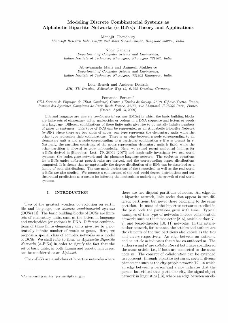
FIG. 1: DNA modeled as a bipartite network α-BiN. The setU consists of 64 codons, whereas the collection V of genes isvirtually infinite. Multiple occurrences of a codon in a genehave been represented here by multi-edges. For instance, thecodons ‘ACG’ and ‘AAU’ have respectively 2 and 3 edgesconnecting to the node gene3. Alternatively, this could havebeen represented by single edges with weights 2 and 3, whilethe weight of the other edges would be equal to 1.

II. THEORETICAL FRAMEWORK FOR α-BINS

A. Formal definition and modeling

A bipartite graph G is a 3-tuple 〈U, V,E〉, where Uand V are mutually exclusive finite collections of nodes(also known as the two partitions) and E ⊆ U × V isthe collection of edges that run between these partitions.We can also define E as a multiset whose elements aredrawn from U×V . Clearly, the last definition of E allowsmultiple edges between a pair of nodes and the numberof times the nodes u ∈ U and v ∈ V are connected canbe assumed to be the weight of the edge (u, v). Note thatalthough we are defining E to be a collection of orderedtuples, the ordering is an implicit outcome of the fact thatedges only run between nodes in U and V . In essence,we do not mean any directedness of the edges.

α-BiNs are a special type of bipartite networks whereone of the partitions represents a set of basic units whilethe other partition represents their combinations. Theset of basic units is essentially finite and fixed over time.Let us denote the unique basic units by the nodes in U .Let each unique discrete combination of the basic unitsbe denoted as a node in V . There exists an edge betweena basic unit u ∈ U and a discrete combination v ∈ V iff u

is a part of v. If u occurs w times in v, then there are wedges between u and v, or alternatively, the weight of theedge (u, v) is w. Fig. 1 illustrates these concepts throughthe example of genes and codons.

Notice that the above model overlooks the order inwhich the basic units are strung into a particular dis-crete combination. The order can be taken into accountby labeling the basic units in order of appearance in eachelement of V . However, in this work, we consider only un-ordered versions of DCSs. As we shall see subsequently,in several real world DCSs, such as the phoneme-languagenetwork, the elements of V are just collections of the el-ements of U , rather than sequences of them.

B. Growth model for sequential attachment

In this subsection, we review the results derived in [22]which apply to sequential as well as parallel attachment.While the results for sequential attachment are exact,for parallel attachment they represent an approximation.In the next subsection the results obtained in [22] areextended and the exact derivation for parallel attachmentis presented.

The growth of α-BiNs is described in terms of a simplemodel based on preferential attachment coupled with atunable randomness parameter. Suppose that the parti-tion U has N nodes labeled as u1 to uN . At each timestep, a new node is introduced in the partition V whichconnects to µ nodes in U based on a predefined attach-ment rule. Let vi be the node added to V during theith time step. The theoretical analysis assumes that µis a constant greater than 0. This constraint will be re-laxed during the construction of the empirical networks.However, note that if the degrees of the nodes in V aresampled from a Poisson-like distribution with mean µ,the theoretical analysis holds good asymptotically.

Let A(kti) be the probability of attaching a new edge

to a node ui, where kti refers to the degree of the node ui

at time t. A(kti) defines the attachment kernel that takes

the form:

A(kti) =

γkti + 1

∑Nj=1(γkt

j + 1)(1)

where the sum in the denominator runs over all the nodesin U , and γ is the tunable parameter which controlsthe relative weight of preferential to random attachment.Thus, the higher the value of γ, the lower the randomnessin the system. Since in a bipartite network the sum of thedegrees of the nodes in the two partitions are equal, thedenominator in the above expression is equal to µγt+N .Note that the numerator of the attachment kernel couldbe rewritten as kt

i + α, where α = 1/γ is a positive con-stant usually referred to as the initial attractiveness [25].

This means that when a new discrete combination, saya gene, enters the system, it is always assumed to haveµ basic units, e.g., a chain of µ codons. The patterns of

4

the codons constituting the newly entered gene dependson the prevalence of the codons in the pre-existing genesas well as a randomness factor 1/γ. At this point it isworthwhile to distinguish between a few basic sub-casesof the growth model. When µ = 1, addition of a nodein V is equivalent to addition of one edge in the net-work and thus the edges attach to the nodes in U in asequential manner. However, for µ > 1 addition of anedge is no longer a sequential process; rather µ edgesare added simultaneously. We refer to the former pro-cess as sequential attachment and the latter as parallelattachment. Depending on the underlying DCS, the par-allel attachment process can be further classified into twosub-cases. If it is required that the µ nodes chosen areall distinct, then we call this parallel attachment with-out replacement. On the other hand, if vi is allowed toattach to the same node more than once, we refer tothe process as parallel attachment with replacement [45].Thus, parallel attachment without replacement leads toα-BiNs without multi-edges or weighted edges, while par-allel attachment with replacement results in α-BiNs withmulti-edges. The two cases collapse for the case of se-quential attachment. To motivate the reader further, weprovide some examples of natural DCSs from each of theaforementioned classes.

• Sequential attachment: Since in the sequential at-tachment model, every node in V has only one edge,there are no discrete combinations at all. Rather,each incoming vi is a reinstantiation of some basicunit uj . However, think of a system where U is theset of languages and V is the collection of speakers,and an edge between u ∈ U and v ∈ V implies thatu is the mother tongue of v. Although not a DCS,these type of “class and its instance” systems areplentiful in nature and can be aptly modeled usingsequential attachment.

• Parallel attachment with replacement: Any DCSmodeled as a sequence of the basic units can bethought to follow the “with replacement” model.For instance, a gene can have many repetitions ofthe same codon and similarly, there may be multi-ple occurrences of the same word in a sentence.

• Parallel attachment without replacement: A DCSthat is a collection of the basic units can be con-ceived as an outcome of the “without replacement”model. For instance, the consonants and vow-els (partition U) that form the repertoire of ba-sic sounds (phonemes) of a language (partition V ),proteins (U) forming protein complexes (V ), etc.

In this work, we focus on the topological propertiesof α-BiNs that are synthesized using the sequential andparallel attachment with replacement. Nevertheless, insection III B we also present some empirical results forthe parallel attachment without replacement model inthe context of the phoneme-language network.

Any α-BiN has two characteristic degree distributionscorresponding to its two partitions U and V . Here weassume that each node in V has degree µ and concentrateon the degree distribution of the nodes in U . Let pk,t bethe probability that a randomly chosen node from thepartition U has degree k after t time steps. We assumethat initially all the nodes in U have a degree 0 and thereare no nodes in V . Therefore,

pk,0 = δk,0 (2)

Here, δ represents the Kronecker symbol. It is interest-ing to note that unlike the case of standard preferentialattachment based growth models for unipartite (e.g., theBA model [18]) and bipartite networks (e.g., [2]), the de-gree distribution of the partition U in α-BiNs cannot besolved using the stationary assumption that in the limitt → ∞, pk,t+1 = pk,t. This is because the average de-gree of the nodes in U , which is µt/N , diverges with t,and consequently, the system does not have a stationarystate.

In [22] it has been shown that pk,t can be approximatedfor µ ≪ N and small values of γ by integrating:

pk,t+1 = (1 − Ap(k, t))pk,t + Ap(k − 1, t)pk−1,t (3)

where Ap(k, t) is defined as

Ap(k, t) =

{(γk+1)µγµt+N for 0 ≤ k ≤ µt

0 otherwise(4)

for t > 0 while for t = 0, Ap(k, t) = (µ/N)δk,0. Thenumerator contains a µ because at each time step thereare µ edges that are being incorporated into the networkrather than a single edge. The solution of Eq. (3) withthe attachment kernel given by Eq. (4) reads:

pk,t =

(tk

) ∏k−1i=0 (γi + 1)

∏t−1−kj=0

(Nµ − 1 + γj

)

∏t−1m=0

(γm + N

µ

) (5)

As already mentioned in [22], Eq. (3) cannot describethe stochastic parallel attachment exactly because it ex-plicitly assumes that in one time step a node of degree kcan only get converted to a node of degree k+1. Clearly,the incorporation of µ edges in parallel allows the possi-bility for a node of degree k to get converted to a nodeof degree k + µ. So, for µ > 1, Eq. (5) is just an approx-imation of the real process for µ ≪ N and small valuesof γ. However, for µ = 1, i.e. for sequential attachment,Eq. (5) is the exact solution of the process.

Interestingly, for γ > 0, Eq. (5) approaches, asymp-totically with time, a beta-distribution as follows.

pk,t ≃ C−1 (k/t)γ−1−1

(1 − k/t)η−γ−1−1

(6)

Here, C is the normalization constant and η = N/(γµ).By making use of the properties of beta distributions, welearn that depending on the value of γ, pk,t can take oneof the following distinctive functional forms.

5

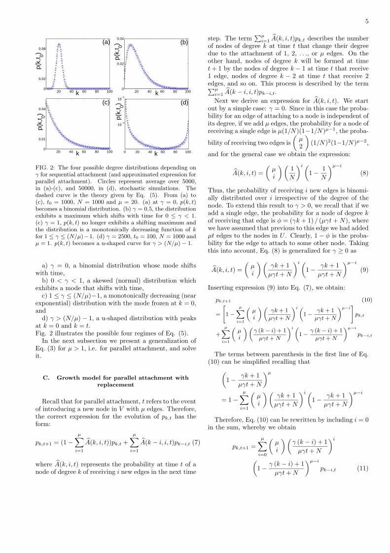
20 40 60 80 1000

0.01

0.04

k

p(k,

t 0)

(c)

0 10020 40 60 80

10−4

10−3

k

p(k,

t 0) (d)

20 40 60 80 1000

0.02

0.08

k

p(k,

t 0)(a)

20 40 60 80 1000

0.02

0.04

k

p(k,

t 0) (b)

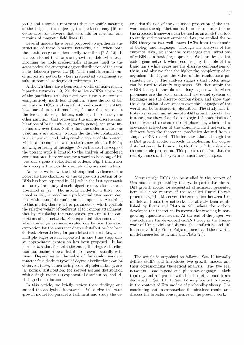
FIG. 2: The four possible degree distributions depending onγ for sequential attachment (and approximated expression forparallel attachment). Circles represent average over 5000,in (a)-(c), and 50000, in (d), stochastic simulations. Thedashed curve is the theory given by Eq. (5). From (a) to(c), t0 = 1000, N = 1000 and µ = 20. (a) at γ = 0, p(k, t)becomes a binomial distribution. (b) γ = 0.5, the distributionexhibits a maximum which shifts with time for 0 ≤ γ < 1.(c) γ = 1, p(k, t) no longer exhibits a shifting maximum andthe distribution is a monotonically decreasing function of kfor 1 ≤ γ ≤ (N/µ)−1. (d) γ = 2500, t0 = 100, N = 1000 andµ = 1. p(k, t) becomes a u-shaped curve for γ > (N/µ) − 1.

a) γ = 0, a binomial distribution whose mode shiftswith time,

b) 0 < γ < 1, a skewed (normal) distribution whichexhibits a mode that shifts with time,

c) 1 ≤ γ ≤ (N/µ)−1, a monotonically decreasing (nearexponential) distribution with the mode frozen at k = 0,and

d) γ > (N/µ) − 1, a u-shaped distribution with peaksat k = 0 and k = t.Fig. 2 illustrates the possible four regimes of Eq. (5).

In the next subsection we present a generalization ofEq. (3) for µ > 1, i.e. for parallel attachment, and solveit.

C. Growth model for parallel attachment withreplacement

Recall that for parallel attachment, t refers to the eventof introducing a new node in V with µ edges. Therefore,the correct expression for the evolution of pk,t has theform:

pk,t+1 = (1 −

µ∑

i=1

A(k, i, t))pk,t +

µ∑

i=1

A(k − i, i, t)pk−i,t (7)

where A(k, i, t) represents the probability at time t of anode of degree k of receiving i new edges in the next time

step. The term∑µ

i=1 A(k, i, t)pk,t describes the numberof nodes of degree k at time t that change their degreedue to the attachment of 1, 2, . . ., or µ edges. On theother hand, nodes of degree k will be formed at timet + 1 by the nodes of degree k − 1 at time t that receive1 edge, nodes of degree k − 2 at time t that receive 2edges, and so on. This process is described by the term∑µ

i=1 A(k − i, i, t)pk−i,t.

Next we derive an expression for A(k, i, t). We startout by a simple case: γ = 0. Since in this case the proba-bility for an edge of attaching to a node is independent ofits degree, if we add µ edges, the probability for a node ofreceiving a single edge is µ(1/N)(1−1/N)µ−1, the proba-

bility of receiving two edges is

(µ2

)(1/N)2(1−1/N)µ−2,

and for the general case we obtain the expression:

A(k, i, t) =

(µi

) (1

N

)i (1 −

1

N

)µ−i

(8)

Thus, the probability of receiving i new edges is binomi-ally distributed over i irrespective of the degree of thenode. To extend this result to γ > 0, we recall that if weadd a single edge, the probability for a node of degree kof receiving that edge is φ = (γk + 1) / (µγt + N), wherewe have assumed that previous to this edge we had addedµt edges to the nodes in U . Clearly, 1 − φ is the proba-bility for the edge to attach to some other node. Takingthis into account, Eq. (8) is generalized for γ ≥ 0 as

A(k, i, t) =

(µi

) (γk + 1

µγt + N

)i (1 −

γk + 1

µγt + N

)µ−i

(9)

Inserting expression (9) into Eq. (7), we obtain:

pk,t+1 (10)

=

"

1 −

µX

i=1

„

µi

« „

γk + 1

µγt + N

«i „

1 −γk + 1

µγt + N

«µ−i#

pk,t

+

µX

i=1

„

µi

« „

γ (k − i) + 1

µγt + N

«i „

1 −γ (k − i) + 1

µγt + N

«µ−i

pk−i,t

The terms between parenthesis in the first line of Eq.(10) can be simplified recalling that

(1 −

γk + 1

µγt + N

)µ

= 1 −

µ∑

i=1

(µi

) (γk + 1

µγt + N

)i (1 −

γk + 1

µγt + N

)µ−i

Therefore, Eq. (10) can be rewritten by including i = 0in the sum, whereby we obtain

pk,t+1 =

µ∑

i=0

(µi

)(γ (k − i) + 1

µγt + N

)i

(1 −

γ (k − i) + 1

µγt + N

)µ−i

pk−i,t (11)

6

0 100 200 300 400 5000

0.01

0.02

0.03

k

p(k,

t=90

0)

0 100 200 300 400 5000

0.01

0.02

0.03

k

p(k,

t=90

0)

(a) (b)

102.5

102.610

−6

10−4

10−2

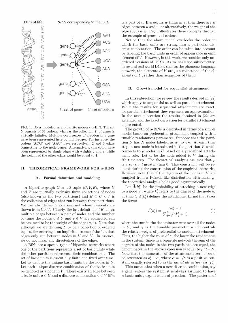
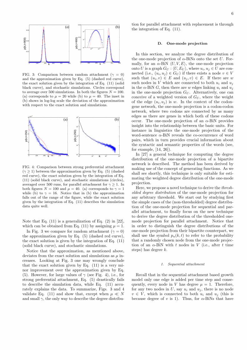
FIG. 3: Comparison between random attachment (γ = 0)and the approximation given by Eq. (5) (dashed red curve),the exact solution given by the integration of Eq. (11) (solidblack curve), and stochastic simulations. Circles correspondto average over 500 simulations. In both the figures N = 100.(a) corresponds to µ = 20 while (b) to µ = 40. The inset in(b) shows in log-log scale the deviation of the approximationwith respect to the exact solution and simulations.

0 100 200 300 400 5000

1

3

5

7

9x 10

−3

k

p(k,

t=25

0)

100

101

102

103

10−4

10−3

10−2

10−1

100

k

p(k,

t=25

0)

(a) (b)

FIG. 4: Comparison between strong preferential attachment(γ ≥ 1) between the approximation given by Eq. (5) (dashedred curve), the exact solution given by the integration of Eq.(11) (solid black curve), and stochastic simulations (circles),averaged over 500 runs, for parallel attachment for γ ≥ 1. Inboth figures N = 100 and µ = 40. (a) corresponds to γ = 1while (b) to γ = 16. Notice that in (b) the approximationfalls out of the range of the figure, while the exact solutiongiven by the integration of Eq. (11) describes the simulationdata quite well.

Note that Eq. (11) is a generalization of Eq. (2) in [22],which can be obtained from Eq. (11) by assigning µ = 1.

In Fig. 3 we compare for random attachment (γ = 0)the approximation given by Eq. (5) (dashed red curve),the exact solution is given by the integration of Eq. (11)(solid black curve), and stochastic simulations.

Notice that the approximation, as mentioned above,deviates from the exact solution and simulations as µ in-creases. Looking at Fig. 3 one may wrongly concludethat the exact solution given by Eq. (11) is a very mi-nor improvement over the approximation given by Eq.(5). However, for large values of γ (see Fig. 4), i.e., forstrong preferential attachment, Eq. (5) drastically failsto describe the simulation data, while Eq. (11) accu-rately explains the data. To summarize, Figs. 3 and 4validate Eq. (11) and show that, except when µ ≪ Nand small γ, the only way to describe the degree distribu-

tion for parallel attachment with replacement is throughthe integration of Eq. (11).

D. One-mode projection

In this section, we analyze the degree distribution ofthe one-mode projection of α-BiNs onto the set U . For-mally, for an α-BiN 〈U, V,E〉, the one-mode projectiononto U is a graph GU : 〈U,EU 〉, where ui, uj ∈ U are con-nected (i.e., (ui, uj) ∈ GU ) if there exists a node v ∈ Vsuch that (ui, v) ∈ E and (uj , v) ∈ E. If there are wsuch nodes in V which are connected to both ui and uj

in the α-BiN G, then there are w edges linking ui and uj

in the one-mode projection GU . Alternatively, one canconceive of a weighted version of GU , where the weightof the edge (ui, uj) is w. In the context of the codon-gene network, the one-mode projection is a codon-codonnetwork, where two codons are connected by as manyedges as there are genes in which both of these codonsoccur. The one-mode projection of an α-BiN providesinsight into the relationship between the basic units. Forinstance in linguistics the one-mode projection of theword-sentence α-BiN reveals the co-occurrence of wordpairs, which in turn provides crucial information aboutthe syntactic and semantic properties of the words (see,for example, [14, 26]).

In [27] a general technique for computing the degreedistribution of the one-mode projection of a bipartitenetwork is described. The method has been derived bymaking use of the concept of generating functions. As weshall see shortly, this technique is only suitable for esti-mating the weighted degree distribution of the one-modeprojection.

Here, we propose a novel technique to derive the thresh-olded degree distribution of the one-mode projection forany arbitrary threshold. We start out by studying firstthe simple cases of the (non-thresholded) degree distribu-tion of the one-mode projection for sequential and par-allel attachment, to finally focus on the new techniqueto derive the degree distribution of the thresholded one-mode projection for parallel attachment. Notice thatin order to distinguish the degree distributions of theone-mode projection from their bipartite counterpart, weshall use the symbol pu(k, t) to refer to the probabilitythat a randomly chosen node from the one-mode projec-tion of an α-BiN with t nodes in V (i.e., after t timesteps) has degree k.

1. Sequential attachment

Recall that in the sequential attachment based growthmodel only one edge is added per time step and conse-quently, every node in V has degree µ = 1. Therefore,for any two nodes in U , say ui and uj , there is no nodev ∈ V , which is connected to both ui and uj (this isbecause degree of v is 1). Thus, for α-BiNs that have

7

0 10 20 30 40 500

0.1

0.2

0.3

0.4

0.5

0.6

0.7

k

p u(k,t)

0 10 20 30 40 500

0.05

0.1

0.15

0.2

0.25

0.3

0.35

0.4

k

p u(k,t)

(a) (b)

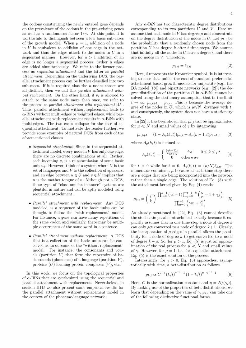
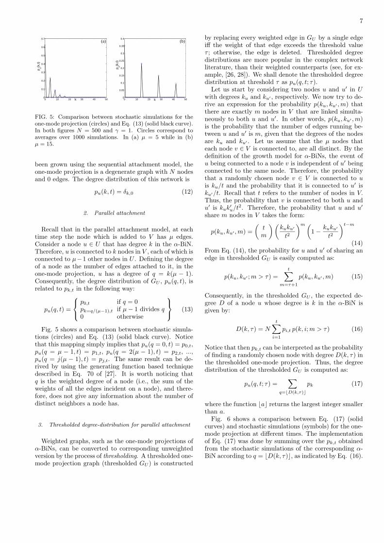
FIG. 5: Comparison between stochastic simulations for theone-mode projection (circles) and Eq. (13) (solid black curve).In both figures N = 500 and γ = 1. Circles correspond toaverages over 1000 simulations. In (a) µ = 5 while in (b)µ = 15.

been grown using the sequential attachment model, theone-mode projection is a degenerate graph with N nodesand 0 edges. The degree distribution of this network is

pu(k, t) = δk,0 (12)

2. Parallel attachment

Recall that in the parallel attachment model, at eachtime step the node which is added to V has µ edges.Consider a node u ∈ U that has degree k in the α-BiN.Therefore, u is connected to k nodes in V , each of which isconnected to µ−1 other nodes in U . Defining the degreeof a node as the number of edges attached to it, in theone-mode projection, u has a degree of q = k(µ − 1).Consequently, the degree distribution of GU , pu(q, t), isrelated to pk,t in the following way:

pu(q, t) =

p0,t if q = 0pk=q/(µ−1),t if µ − 1 divides q0 otherwise

(13)

Fig. 5 shows a comparison between stochastic simula-tions (circles) and Eq. (13) (solid black curve). Noticethat this mapping simply implies that pu(q = 0, t) = p0,t,pu(q = µ − 1, t) = p1,t, pu(q = 2(µ − 1), t) = p2,t, ...,pu(q = j(µ − 1), t) = pj,t. The same result can be de-rived by using the generating function based techniquedescribed in Eq. 70 of [27]. It is worth noticing thatq is the weighted degree of a node (i.e., the sum of theweights of all the edges incident on a node), and there-fore, does not give any information about the number ofdistinct neighbors a node has.

3. Thresholded degree-distribution for parallel attachment

Weighted graphs, such as the one-mode projections ofα-BiNs, can be converted to corresponding unweightedversion by the process of thresholding. A thresholded one-mode projection graph (thresholded GU ) is constructed

by replacing every weighted edge in GU by a single edgeiff the weight of that edge exceeds the threshold valueτ ; otherwise, the edge is deleted. Thresholded degreedistributions are more popular in the complex networkliterature, than their weighted counterparts (see, for ex-ample, [26, 28]). We shall denote the thresholded degreedistribution at threshold τ as pu(q, t; τ).

Let us start by considering two nodes u and u′ in Uwith degrees ku and ku′ , respectively. We now try to de-rive an expression for the probability p(ku, ku′ ,m) thatthere are exactly m nodes in V that are linked simulta-neously to both u and u′. In other words, p(ku, ku′ ,m)is the probability that the number of edges running be-tween u and u′ is m, given that the degrees of the nodesare ku and ku′ . Let us assume that the µ nodes thateach node v ∈ V is connected to, are all distinct. By thedefinition of the growth model for α-BiNs, the event ofu being connected to a node v is independent of u′ beingconnected to the same node. Therefore, the probabilitythat a randomly chosen node v ∈ V is connected to uis ku/t and the probability that it is connected to u′ isku′/t. Recall that t refers to the number of nodes in V.Thus, the probability that v is connected to both u andu′ is kuk′

u/t2. Therefore, the probability that u and u′

share m nodes in V takes the form:

p(ku, ku′ ,m) =

(tm

)(kuku′

t2

)m (1 −

kuku′

t2

)t−m

(14)From Eq. (14), the probability for u and u′ of sharing anedge in thresholded GU is easily computed as:

p(ku, ku′ ;m > τ) =

t∑

m=τ+1

p(ku, ku′ ,m) (15)

Consequently, in the thresholded GU , the expected de-gree D of a node u whose degree is k in the α-BiN isgiven by:

D(k, τ) = N

t∑

i=1

pi,t p(k, i;m > τ) (16)

Notice that then pk,t can be interpreted as the probabilityof finding a randomly chosen node with degree D(k, τ) inthe thresholded one-mode projection. Thus, the degreedistribution of the thresholded GU is computed as:

pu(q, t; τ) =∑

q=⌊D(k,τ)⌋

pk (17)

where the function ⌊a⌋ returns the largest integer smallerthan a.

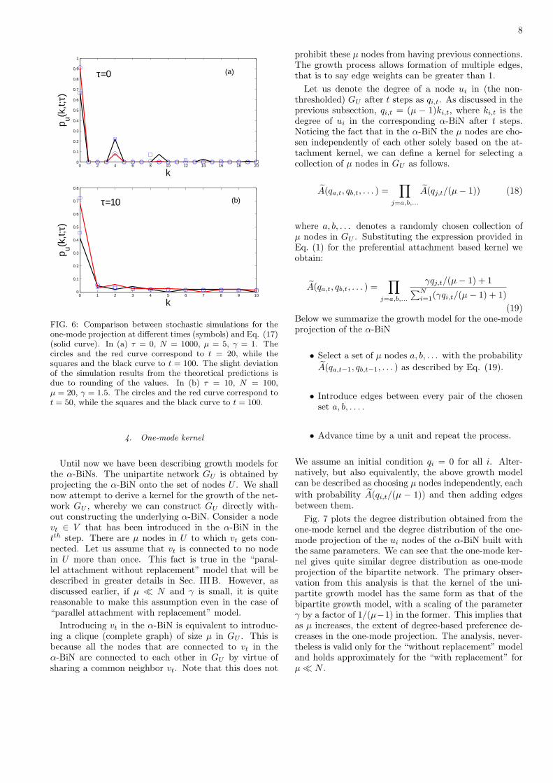
Fig. 6 shows a comparison between Eq. (17) (solidcurves) and stochastic simulations (symbols) for the one-mode projection at different times. The implementationof Eq. (17) was done by summing over the pk,t obtainedfrom the stochastic simulations of the corresponding α-BiN according to q = ⌊D(k, τ)⌋, as indicated by Eq. (16).

8

0 2 4 6 8 10 12 14 16 18 200

0.1

0.2

0.3

0.4

0.5

0.6

0.7

0.8

0.9

1

k

p u(k,t;

τ)τ=0 (a)

0 1 2 3 4 5 6 7 8 9 100

0.1

0.2

0.3

0.4

0.5

0.6

0.7

0.8

k

p u(k,t;

τ)

τ=10 (b)

FIG. 6: Comparison between stochastic simulations for theone-mode projection at different times (symbols) and Eq. (17)(solid curve). In (a) τ = 0, N = 1000, µ = 5, γ = 1. Thecircles and the red curve correspond to t = 20, while thesquares and the black curve to t = 100. The slight deviationof the simulation results from the theoretical predictions isdue to rounding of the values. In (b) τ = 10, N = 100,µ = 20, γ = 1.5. The circles and the red curve correspond tot = 50, while the squares and the black curve to t = 100.

4. One-mode kernel

Until now we have been describing growth models forthe α-BiNs. The unipartite network GU is obtained byprojecting the α-BiN onto the set of nodes U . We shallnow attempt to derive a kernel for the growth of the net-work GU , whereby we can construct GU directly with-out constructing the underlying α-BiN. Consider a nodevt ∈ V that has been introduced in the α-BiN in thetth step. There are µ nodes in U to which vt gets con-nected. Let us assume that vt is connected to no nodein U more than once. This fact is true in the “paral-lel attachment without replacement” model that will bedescribed in greater details in Sec. III B. However, asdiscussed earlier, if µ ≪ N and γ is small, it is quitereasonable to make this assumption even in the case of“parallel attachment with replacement” model.

Introducing vt in the α-BiN is equivalent to introduc-ing a clique (complete graph) of size µ in GU . This isbecause all the nodes that are connected to vt in theα-BiN are connected to each other in GU by virtue ofsharing a common neighbor vt. Note that this does not

prohibit these µ nodes from having previous connections.The growth process allows formation of multiple edges,that is to say edge weights can be greater than 1.

Let us denote the degree of a node ui in (the non-thresholded) GU after t steps as qi,t. As discussed in theprevious subsection, qi,t = (µ − 1)ki,t, where ki,t is thedegree of ui in the corresponding α-BiN after t steps.Noticing the fact that in the α-BiN the µ nodes are cho-sen independently of each other solely based on the at-tachment kernel, we can define a kernel for selecting acollection of µ nodes in GU as follows.

A(qa,t, qb,t, . . . ) =∏

j=a,b,...

A(qj,t/(µ − 1)) (18)

where a, b, . . . denotes a randomly chosen collection ofµ nodes in GU . Substituting the expression provided inEq. (1) for the preferential attachment based kernel weobtain:

A(qa,t, qb,t, . . . ) =∏

j=a,b,...

γqj,t/(µ − 1) + 1∑N

i=1(γqi,t/(µ − 1) + 1)

(19)Below we summarize the growth model for the one-modeprojection of the α-BiN

• Select a set of µ nodes a, b, . . . with the probability

A(qa,t−1, qb,t−1, . . . ) as described by Eq. (19).

• Introduce edges between every pair of the chosenset a, b, . . . .

• Advance time by a unit and repeat the process.

We assume an initial condition qi = 0 for all i. Alter-natively, but also equivalently, the above growth modelcan be described as choosing µ nodes independently, each

with probability A(qi,t/(µ − 1)) and then adding edgesbetween them.

Fig. 7 plots the degree distribution obtained from theone-mode kernel and the degree distribution of the one-mode projection of the ui nodes of the α-BiN built withthe same parameters. We can see that the one-mode ker-nel gives quite similar degree distribution as one-modeprojection of the bipartite network. The primary obser-vation from this analysis is that the kernel of the uni-partite growth model has the same form as that of thebipartite growth model, with a scaling of the parameterγ by a factor of 1/(µ−1) in the former. This implies thatas µ increases, the extent of degree-based preference de-creases in the one-mode projection. The analysis, never-theless is valid only for the “without replacement” modeland holds approximately for the “with replacement” forµ ≪ N .

9

0 50 100 1500

0.02

0.04

0.06

0.08

k

p(k)

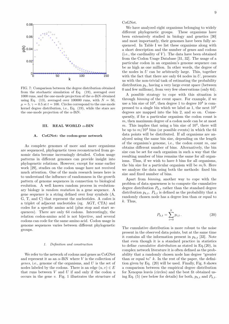
FIG. 7: Comparison between the degree distribution obtainedfrom the stochastic simulation of Eq. (19), averaged over1000 runs, and the one-mode projection of the α-BiN obtainedusing Eq. (13), averaged over 100000 runs, with N = 50,µ = 5, γ = 0.5 at t = 100. Circles correspond to the one-modekernel degree distribution, i.e., Eq. (19), while the stars arethe one-mode projection of the α-BiN.

III. REAL WORLD α-BIN

A. CoGNet: the codon-gene network

As complete genomes of more and more organismsare sequenced, phylogenetic trees reconstructed from ge-nomic data become increasingly detailed. Codon usagepatterns in different genomes can provide insight intophylogenetic relations. However, except for some earlierwork [29], studies on the codon usage have not receivedmuch attention. One of the main research issues here isto understand the influence of randomness in the growthpattern of genome sequences in connection to biologicalevolution. A well known random process in evolution-ary biology is random mutation in a gene sequence. Agene sequence is a string defined over four symbols (A,G, T, and C) that represent the nucleotides. A codon isa triplet of adjacent nucleotides (eg. AGT, CTA) andcodes for a specific amino acid (plus stop and start se-quences). There are only 64 codons. Interestingly, therelation codon-amino acid is not bijective, and severalcodons can code for the same amino acid. Codon usage ingenome sequences varies between different phylogeneticgroups.

1. Definition and construction

We refer to the network of codons and genes as CoGNetand represent it as an α-BiN where V is the collection ofgenes, i.e., genome of the organisms, and U is the set ofnodes labeled by the codons. There is an edge (u, v) ∈ Ethat runs between V and U if and only if the codon uoccurs in the gene v. Fig. 1 illustrates the structure of

CoGNet.

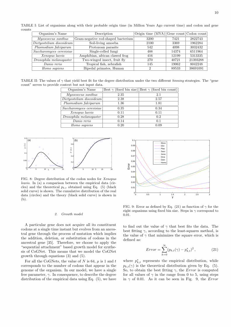
We have analyzed eight organisms belonging to widelydifferent phylogenetic groups. These organisms havebeen extensively studied in biology and genetics [30]and most importantly, their genomes have been fully se-quenced. In Table I we list these organisms along witha short description and the number of genes and codons(i.e., the cardinality of V ). The data have been obtainedfrom the Codon Usage Database [31, 32]. The usage of aparticular codon in an organism’s genome sequence canbe as high as one million. In other words, the degree ofthe nodes in U can be arbitrarily large. This, togetherwith the fact that there are only 64 nodes in U , presentsus with the non-trivial task of estimating the probabilitydistribution pk, having a very large event space (between0 and few millions), from very few observations (only 64).

A possible strategy to cope with this situation isthrough binning of the event space. For example, if weuse a bin size of 104, then degree 1 to degree 104 is com-pressed to a single bin which we label as 1, the next 104

degrees are mapped into the bin 2, and so on. Conse-quently, if for a particular organism the codon count ism, then maximum degree of a codon node can be at mostm. This implies that using a bin size of 104, there willbe up to m/104 bins (or possible events) in which the 64data points will be distributed. If all organisms are an-alyzed using the same bin size, depending on the lengthof the organism’s genome, i.e., the codon count m, oneobtains different number of bins. Alternatively, the binsize can be set for each organism in such a way that theresulting number of bins remains the same for all organ-isms. Thus, if we wish to have b bins for all organisms,the bin size for a particular organism will be m/b. Herewe analyze the data using both the methods: fixed binsize and fixed number of bins.

Apart from binning, another way to cope with theproblem of data sparseness is to compute the cumulativedegree distribution Pk,t rather than the standard degreedistribution pk,t. Pk,t is defined as the probability that arandomly chosen node has a degree less than or equal tok. Thus,

Pk,t =

k∑

i=0

pi,t . (20)

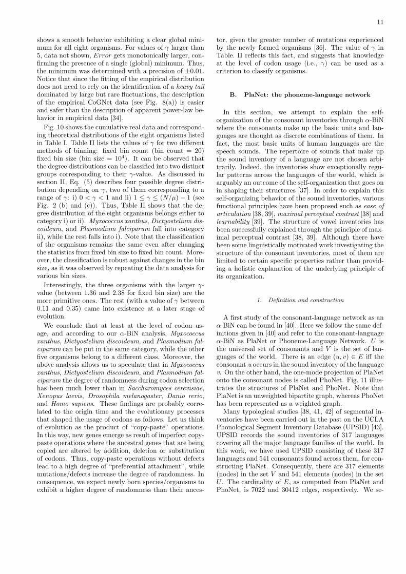
The cumulative distribution is more robust to the noisepresent in the observed data points, but at the same timeit contains all the information present in pk,t [33]. Notethat even though it is a standard practice in statisticsto define cumulative distribution as stated in Eq.(20), incomplex network literature it is often defined as the prob-ability that a randomly chosen node has degree “greaterthan or equal to” k. In the rest of the paper, the defini-tion given by Eq. (20) will be used. Finally, Fig. 8 showsa comparison between the empirical degree distributionfor Xenopus leavis (circles) and the best fit obtained us-ing Eq. (5) (see below for details) for both, pk,t and Pk,t.

10

TABLE I: List of organisms along with their probable origin time (in Million Years Ago current time) and codon and genecounts

Organism’s Name Description Origin time (MYA) Gene count Codon count

Myxococcus xanthus Gram-negative rod-shaped bacterium 3200 7421 2822743Dictyostelium discoideum Soil-living amoeba 2100 3369 1962284Plasmodium falciparum Protozoan parasite 542 4098 3032432Saccharomyces cerevisiae Single-celled fungi 488 14374 6511964

Xenopus laevis Amphibian, african clawed frog 416 12199 5313335Drosophila melanogaster Two-winged insect, fruit fly 270 40721 21393288

Danio rerio Tropical fish, zebrafish 145 19062 8042248Homo sapiens Bipedal primates, Human 2 89533 38691091

TABLE II: The values of γ that yield best fit for the degree distribution under the two different binning strategies. The “genecount” serves to provide context but not input data.

Organism’s Name Best γ (fixed bin size) Best γ (fixed bin count)

Myxococcus xanthus 2.35 2.1Dictyostelium discoideum 2.38 2.57Plasmodium falciparum 1.36 1.81

Saccharomyces cerevisiae 0.35 0.34Xenopus laevis 0.11 0.11

Drosophila melanogaster 0.28 0.2Danio rerio 0.14 0.1

Homo sapiens 0.20 0.09

0 5 10 15 200

0.05

0.1

0.2

k

p(k)

(a)

0 5 10 15 200

0.2

0.4

0.8

1

k

P(k)

(b)

FIG. 8: Degree distribution of the codon nodes for Xenopusleavis. In (a) a comparison between the empirical data (cir-cles) and the theoretical pk,t obtained using Eq. (5) (blacksolid curve) is shown. The cumulative distribution of the realdata (circles) and the theory (black solid curve) is shown in(b).

2. Growth model

A particular gene does not acquire all its constituentcodons at a single time instant but evolves from an ances-tral gene through the process of mutation which impliesthe addition, deletion, or substitution of codons in theancestral gene [35]. Therefore, we choose to apply the“sequential attachment” based growth model for synthe-sis of CoGNet. This means that we model the CoGNetgrowth through equations (3) and (5).

For all the CoGNets, the value of N is 64, µ is 1 and tcorresponds to the number of codons that appear in thegenome of the organism. In our model, we have a singlefree parameter, γ. In consequence, to describe the degreedistribution of the empirical data using Eq. (5), we have

0 0.5 1 1.5 2 2.5 30

0.01

0.02

0.03

0.04

0.05

0.06

0.07

0.08

0.09

0.1

γ

Err

or

MyxoDictPlasSaccXenoDrosDaniHomo

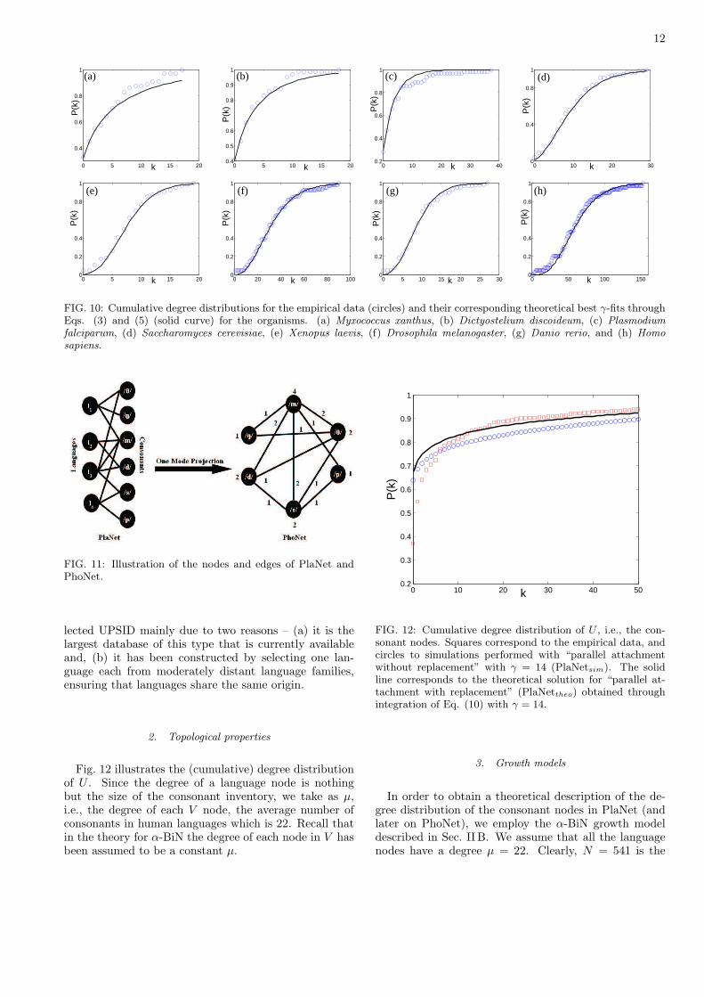
FIG. 9: Error as defined by Eq. (21) as function of γ for theeight organisms using fixed bin size. Steps in γ correspond to0.01.

to find out the value of γ that best fits the data. Thebest fitting γ, according to the least-squares method, isthe value of γ that minimizes the square error, which isdefined as:

Error =∞∑

k=0

(pk,t(γ) − p∗k,t)2 , (21)

where p∗k,t represents the empirical distribution, while

pk,t(γ) is the theoretical distribution given by Eq. (5).So, to obtain the best fitting γ, the Error is computedfor all values of γ in the range from 0 to 5, using stepsin γ of 0.01. As it can be seen in Fig. 9, the Error

11

shows a smooth behavior exhibiting a clear global mini-mum for all eight organisms. For values of γ larger than5, data not shown, Error gets monotonically larger, con-firming the presence of a single (global) minimum. Thus,the minimum was determined with a precision of ±0.01.Notice that since the fitting of the empirical distributiondoes not need to rely on the identification of a heavy taildominated by large but rare fluctuations, the descriptionof the empirical CoGNet data (see Fig. 8(a)) is easierand safer than the description of apparent power-law be-havior in empirical data [34].

Fig. 10 shows the cumulative real data and correspond-ing theoretical distributions of the eight organisms listedin Table I. Table II lists the values of γ for two differentmethods of binning: fixed bin count (bin count = 20)fixed bin size (bin size = 104). It can be observed thatthe degree distributions can be classified into two distinctgroups corresponding to their γ-value. As discussed insection II, Eq. (5) describes four possible degree distri-bution depending on γ, two of them corresponding to arange of γ: i) 0 < γ < 1 and ii) 1 ≤ γ ≤ (N/µ) − 1 (seeFig. 2 (b) and (c)). Thus, Table II shows that the de-gree distribution of the eight organisms belongs either tocategory i) or ii). Myxococcus xanthus, Dictyostelium dis-coideum, and Plasmodium falciparum fall into categoryii), while the rest falls into i). Note that the classificationof the organisms remains the same even after changingthe statistics from fixed bin size to fixed bin count. More-over, the classification is robust against changes in the binsize, as it was observed by repeating the data analysis forvarious bin sizes.

Interestingly, the three organisms with the larger γ-value (between 1.36 and 2.38 for fixed bin size) are themore primitive ones. The rest (with a value of γ between0.11 and 0.35) came into existence at a later stage ofevolution.

We conclude that at least at the level of codon us-age, and according to our α-BiN analysis, Myxococcusxanthus, Dictyostelium discoideum, and Plasmodium fal-ciparum can be put in the same category, while the otherfive organisms belong to a different class. Moreover, theabove analysis allows us to speculate that in Myxococcusxanthus, Dictyostelium discoideum, and Plasmodium fal-ciparum the degree of randomness during codon selectionhas been much lower than in Saccharomyces cerevisiae,Xenopus laevis, Drosophila melanogaster, Danio rerio,and Homo sapiens. These findings are probably corre-lated to the origin time and the evolutionary processesthat shaped the usage of codons as follows. Let us thinkof evolution as the product of “copy-paste” operations.In this way, new genes emerge as result of imperfect copy-paste operations where the ancestral genes that are beingcopied are altered by addition, deletion or substitutionof codons. Thus, copy-paste operations without defectslead to a high degree of “preferential attachment”, whilemutations/defects increase the degree of randomness. Inconsequence, we expect newly born species/organisms toexhibit a higher degree of randomness than their ances-

tor, given the greater number of mutations experiencedby the newly formed organisms [36]. The value of γ inTable. II reflects this fact, and suggests that knowledgeat the level of codon usage (i.e., γ) can be used as acriterion to classify organisms.

B. PlaNet: the phoneme-language network

In this section, we attempt to explain the self-organization of the consonant inventories through α-BiNwhere the consonants make up the basic units and lan-guages are thought as discrete combinations of them. Infact, the most basic units of human languages are thespeech sounds. The repertoire of sounds that make upthe sound inventory of a language are not chosen arbi-trarily. Indeed, the inventories show exceptionally regu-lar patterns across the languages of the world, which isarguably an outcome of the self-organization that goes onin shaping their structures [37]. In order to explain thisself-organizing behavior of the sound inventories, variousfunctional principles have been proposed such as ease ofarticulation [38, 39], maximal perceptual contrast [38] andlearnability [39]. The structure of vowel inventories hasbeen successfully explained through the principle of max-imal perceptual contrast [38, 39]. Although there havebeen some linguistically motivated work investigating thestructure of the consonant inventories, most of them arelimited to certain specific properties rather than provid-ing a holistic explanation of the underlying principle ofits organization.

1. Definition and construction

A first study of the consonant-language network as anα-BiN can be found in [40]. Here we follow the same def-initions given in [40] and refer to the consonant-languageα-BiN as PlaNet or Phoneme-Language Network. U isthe universal set of consonants and V is the set of lan-guages of the world. There is an edge (u, v) ∈ E iff theconsonant u occurs in the sound inventory of the languagev. On the other hand, the one-mode projection of PlaNetonto the consonant nodes is called PhoNet. Fig. 11 illus-trates the structures of PlaNet and PhoNet. Note thatPlaNet is an unweighted bipartite graph, whereas PhoNethas been represented as a weighted graph.

Many typological studies [38, 41, 42] of segmental in-ventories have been carried out in the past on the UCLAPhonological Segment Inventory Database (UPSID) [43].UPSID records the sound inventories of 317 languagescovering all the major language families of the world. Inthis work, we have used UPSID consisting of these 317languages and 541 consonants found across them, for con-structing PlaNet. Consequently, there are 317 elements(nodes) in the set V and 541 elements (nodes) in the setU . The cardinality of E, as computed from PlaNet andPhoNet, is 7022 and 30412 edges, respectively. We se-

12

0 5 10 15 20

0.4

0.6

0.8

1

k

P(k

)(a)

0 5 10 15 200.4

0.5

0.6

0.8

0.9

1

k

P(k

)

(b)

0 10 20 30 400.2

0.4

0.6

0.8

1

k

P(k

)

(c)

0 10 20 300

0.4

0.8

1

k

P(k

)

(d)

0 5 10 15 200

0.2

0.4

0.8

1

k

P(k

)

(e)

0 20 40 60 80 1000

0.2

0.4

0.8

1

k

P(k

)

(f)

0 5 10 15 20 25 300

0.2

0.4

0.8

1

k

P(k

)

(g)

0 50 100 1500

0.2

0.4

0.8

1

k

P(k

)

(h)

FIG. 10: Cumulative degree distributions for the empirical data (circles) and their corresponding theoretical best γ-fits throughEqs. (3) and (5) (solid curve) for the organisms. (a) Myxococcus xanthus, (b) Dictyostelium discoideum, (c) Plasmodiumfalciparum, (d) Saccharomyces cerevisiae, (e) Xenopus laevis, (f) Drosophila melanogaster, (g) Danio rerio, and (h) Homosapiens.

FIG. 11: Illustration of the nodes and edges of PlaNet andPhoNet.

lected UPSID mainly due to two reasons – (a) it is thelargest database of this type that is currently availableand, (b) it has been constructed by selecting one lan-guage each from moderately distant language families,ensuring that languages share the same origin.

2. Topological properties

Fig. 12 illustrates the (cumulative) degree distributionof U . Since the degree of a language node is nothingbut the size of the consonant inventory, we take as µ,i.e., the degree of each V node, the average number ofconsonants in human languages which is 22. Recall thatin the theory for α-BiN the degree of each node in V hasbeen assumed to be a constant µ.

0 10 20 30 40 500.2

0.3

0.4

0.5

0.6

0.7

0.8

0.9

1

k

P(k

)

FIG. 12: Cumulative degree distribution of U , i.e., the con-sonant nodes. Squares correspond to the empirical data, andcircles to simulations performed with “parallel attachmentwithout replacement” with γ = 14 (PlaNetsim). The solidline corresponds to the theoretical solution for “parallel at-tachment with replacement” (PlaNettheo) obtained throughintegration of Eq. (10) with γ = 14.

3. Growth models

In order to obtain a theoretical description of the de-gree distribution of the consonant nodes in PlaNet (andlater on PhoNet), we employ the α-BiN growth modeldescribed in Sec. II B. We assume that all the languagenodes have a degree µ = 22. Clearly, N = 541 is the

13

total number of consonant nodes and t = 317 is the to-tal number of languages. Thus, γ is the only free pa-rameter in the model. Notice that, by definition, inPlaNet a consonant can occur only once in a languageinventory. Therefore, unlike the case of CoGNet, PlaNetis an α-BiN that has been constructed using a “paral-lel attachment without replacement” scheme. However,we expect the theory developed in Sec. II B, correspond-ing to “parallel attachment with replacement”, to be afairly good approximation for the degree distribution ofPlaNet. We shall refer this theoretical model of PlaNetas PlaNettheo. In order to estimate the free parameter γ,the best fit was obtained with γ = 14 (see Fig. 12). Since1 ≤ γ ≤ N/µ = 24.6, based on our theoretical analysiswe can conclude that the degree distribution is consistentwith an attachment kernel where preferetial attachmenthas a strong weight, i.e., γ takes a large value. Conse-quently, the degree distribution is consistent with a betadistribution, exhibiting its mode at k = 1.

To study the effect of the “parallel attachment with-out replacement” scheme, we carry out stochastic simu-lations with such a growth model described below. Sup-pose that a language node vi (with degree 22) is addedto the system and that j < 22 edges of the incomingnode have already been attached to u1, u2, ..., uj distinctconsonant nodes. Then, the (j + 1)th edge is attachedto a consonant node based on the same preferential at-tachment kernel (see Eq. 1), but applied on the re-duced set U−{u1, u2, . . . , uj}, i.e., the previously selectedu1, u2, ..., uj consonant nodes cannot participate in theselection process of the (j +1)th edge of vi. This ensuresthat a consonant node is never chosen twice. We shallrefer to the degree distributions of the consonant nodesobtained in this way as PlaNetsim. The degree distri-bution of PlaNetsim has the best match with the degreedistribution of the real PlaNet when γ = 14.

We have calculated the error for the aforementionedstochastic simulation model (Esim) as well as the theoryof Sec. II B, corresponding to “parallel attachment withreplacement” (Etheo). The error has been computed us-ing Eq. (21) where p∗k,t stands for the degree distributionof the real PlaNet. It is found that Esim = 0.0972 andEtheo = 0.1170. Since the simulation using the “par-allel attachment without replacement” scheme describesthe structure of consonant inventories better, the errorin this case is smaller than that for “parallel attachmentwith replacement”.

4. One-mode projection: PhoNet

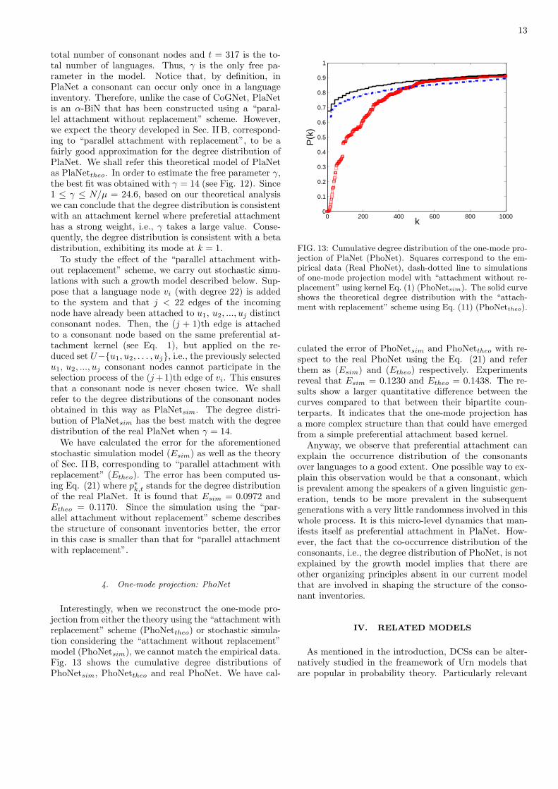
Interestingly, when we reconstruct the one-mode pro-jection from either the theory using the “attachment withreplacement” scheme (PhoNettheo) or stochastic simula-tion considering the “attachment without replacement”model (PhoNetsim), we cannot match the empirical data.Fig. 13 shows the cumulative degree distributions ofPhoNetsim, PhoNettheo and real PhoNet. We have cal-

0 200 400 600 800 10000

0.1

0.2

0.3

0.4

0.5

0.6

0.7

0.8

0.9

1

k

P(k

)

FIG. 13: Cumulative degree distribution of the one-mode pro-jection of PlaNet (PhoNet). Squares correspond to the em-pirical data (Real PhoNet), dash-dotted line to simulationsof one-mode projection model with “attachment without re-placement” using kernel Eq. (1) (PhoNetsim). The solid curveshows the theoretical degree distribution with the “attach-ment with replacement” scheme using Eq. (11) (PhoNettheo).

culated the error of PhoNetsim and PhoNettheo with re-spect to the real PhoNet using the Eq. (21) and referthem as (Esim) and (Etheo) respectively. Experimentsreveal that Esim = 0.1230 and Etheo = 0.1438. The re-sults show a larger quantitative difference between thecurves compared to that between their bipartite coun-terparts. It indicates that the one-mode projection hasa more complex structure than that could have emergedfrom a simple preferential attachment based kernel.

Anyway, we observe that preferential attachment canexplain the occurrence distribution of the consonantsover languages to a good extent. One possible way to ex-plain this observation would be that a consonant, whichis prevalent among the speakers of a given linguistic gen-eration, tends to be more prevalent in the subsequentgenerations with a very little randomness involved in thiswhole process. It is this micro-level dynamics that man-ifests itself as preferential attachment in PlaNet. How-ever, the fact that the co-occurrence distribution of theconsonants, i.e., the degree distribution of PhoNet, is notexplained by the growth model implies that there areother organizing principles absent in our current modelthat are involved in shaping the structure of the conso-nant inventories.

IV. RELATED MODELS

As mentioned in the introduction, DCSs can be alter-natively studied in the freamework of Urn models thatare popular in probability theory. Particularly relevant

14

to us is the so-called Finite Polya’s process [23, 24]. Theprocess is defined as follows:

1) Imagine a system consisting of N bins, each of themcontaining one ball at time t = 0,

2) at the time step t + 1, place a new ball in the i-th bin with a probability proportional to nη

i (t), whereni(t) is the number of balls in i-th bin at time t, and theexponent η is a model parameter.

The Finite Polya’s process is closely related to the de-veloped α-BiN growth model for sequential attachmentwith µ = 1. However, there are several differences. Forinstance, notice that by definition Polya’s process re-quires step 1), which means every bin is assumed to haveone ball at time t = 0. In contrast, in the α-BiN growthmodel we can assume any initial condition. In particu-lar, we have studied the case where at t = 0, all bins areempty, because in the α-BiN growth model the probabil-ity of getting a new ball is proportional to γni(t) + 1.Defining this probability as consisting of two additiveterms has another advantage – we can change γ, thatis our model parameter, so as to control the weight be-tween both the terms. It is easy to see that if in the step1) of the Finite Polya’s process the urns are assumed tocontain 1/γ balls instead of one ball, then this modifiedprocess, and for η = 1, exactly corresponds to the α-BiN

model, under the mapping nαBiNi 7→ nPolya

i − 1/γ. Nev-ertheless, this generalization, whereby we control the na-ture of the emergent degree distribution by varying theparameter γ has not been studied previously. Instead,the shape of the urn-size distribution (equivalent to de-gree distribution in α-BiNs) in a Finite Polya’s process iscontrolled by varying η. It is important to notice that theuse of a linear attachment probability has allowed us toobtain an analytical closed form for the case of sequen-tial attachment, and to derive the exact expression forthe time evolution of the degree distribution for parallelattachment, which is not the case for the Finite Polya’sprocess. The use of a non-linear attachment probabilitymakes the analytical treatment of the latter model muchmore difficult. However, we stress that it could be in-teresting to explore the α-BiN growth model that resultsfrom combining both degrees of freedom, η and γ, in sucha way that the attachment probability becomes propor-tional to γnη

i (t) + 1. Though in this case the analyticaltreatment of the problem becomes much more involved,it is possible that such a treatment could explain the em-pirical data more accurately.

Finally, there is another important difference betweenPolya’s and α-BiN growth models that is worth mention-ing. While Polya’s urn model is defined in such a waythat at each time step only one ball enters into the sys-tem, in the α-BiN growth model µ balls are added intothe system per time step. As extensively discussed insection II, the solutions of the problem are remarkablydifferent when the µ balls are added sequentially or inparallel to the system.

Another class of models for non-growing bipartite net-works developed by Evans and Plato in [20] (henceforth

the EP Model) is based on the concept of rewiring andclosely resemble the Urn model. In this study, one of thepartitions, which the authors refer to as the set of arti-facts, is fixed. The nodes in the other partition are re-ferred to as individuals, all of which have degree one. Thenames artifacts and individuals reflect the fact that themodel was initially conceived to describe cultural trans-mission. Note that artifacts and individuals are com-parable, in the context of an α-BiN to the basic unitsand their discrete combinations, respectively. In the EPmodel there are fixed number of edges. At every timestep, an artifact node is selected following a distributionΠR and an edge that is connected to the chosen artifactis picked up at random. This edge is then rewired to an-other artifact node which is chosen according to a distri-bution ΠA. During the rewiring process the other end ofthe edge is always attached to the same individual node.The authors derive the exact analytical expressions forthe degree distribution of the artifact nodes at all timesand for all values of the parameters for the following def-initions of the removal and attachment probabilities:

ΠR =k

E, ΠA = pr

1

N+ pp

k

E

where E, N and k stands for the number of edges, thenumber of artifacts, and the degree of an artifact node,respectively. Furthermore, pr and pp, which add up toone, are positive constants (model parameters) that con-trol the balance between random and preferential attach-ment.

The EP model is comparable to the α-BiN growthmodel for sequential attachment, except for the fact thatthe total number of edges in the latter case divergeswith time, which changes the scenario completely. Ifwe rewrite the attachment probability for the sequentialgrowth model in a form similar to that of ΠA, we obtainthe following expressions for the parameters pr and pp.

pr =1

1 + γt/N, pp =

γt/N

1 + γt/N

Clearly, as t → ∞, pr → 0 and pp → 1, whereas in theEP model these parameters are fixed. Thus, apart fromthe two extreme cases of pr = 0 and pr = 1, the twomodels are fundamentally different, a fact which is alsomanifested in their emergent degree distributions. Forinstance, in EP model the distributions reach a steadystate, while this does not occur in α-BiNs. In addition,while for α-BiNs, we observe four distinct types of degreedistributions, the equilibrium degree distribution of theEP model shows only two patterns: inverse power-lawwith exponential cut off (comparable to the case whenγ < 1), and a u-shaped distribution (comparable to thecase of very large γ).

15

V. DISCUSSION AND CONCLUSION

In the preceding sections, we have presented growthmodels for discrete combinatorial systems in the frame-work of a special class of networks – α-BiNs. To summa-rize some of our important contributions, we have

• proposed growth models for α-BiNs, which arebased on preferential attachment coupled with atunable randomness component,

• extended the mathematical analysis presentedin [22] and derived the exact expression for the de-gree distribution in case of parallel attachment,

• analytically derived the degree distribution of theone-mode projection,

• and presented case studies for two well-knownDCSs from the domain of biology and language, inorder to illustrate how to apply our analytical find-ings to describe the empirical data, and to discussthe limitations of α-BiNs as a modeling tool.

A natural generalization of the α-BiN growth modelsintroduced here would involve the use of non-linear at-tachment kernels, as discussed above, and the modelingof rewiring during the growth of the α-BiN . In fact,it has been shown through simulations that the degreedistribution of the consonant nodes in PlaNet is betterexplained by having a superlinear kernel as opposed toa linear kernel presented here [44]. An analytical treat-ment of such a non-linear kernel should be an interestingtopic for future research.

There are also some limitations in the study ofCoGNet. Selection of correct binning policy to construct

the CoGNet is a challenging job. Modeling the CoGNetwith parallel attachment where µ is the average numberof codons present in the genes is a direct extension ofthe current work. As a first step, we here classified theeight organisms into two sets and we believe that ournew method can further contribute to the reconstructionof phylogenetic relations. Our approach may be espe-cially useful for the analysis of such genome sequenceswhich are so far only available in fragments either dueto fragmentary sampling of the biological material or toun-finished sequencing efforts.

Finally, we would like to argue that the condition thatone of the partitions in the α-BiN model has to be strictlyfixed in size can be relaxed. It is possible to find some realsystems where the set of basic units also grow, althoughat a far slower rate than the collection of their discretecombinations. Under this condition we can expect the re-ported results to approximately hold. However, it wouldbe very interesting to study to what extent the rate ofgrowth of the two partitions should differ for the currenttheoretical predictions to remain valid.

Acknowledgments

This work was partially financed by the Indo-Germancollaboration project DST-BMBT through grant “Devel-oping robust and efficient services for open source Inter-net telephony over peer to peer network”. N.G., A.N.M.and A.M. acknowledge the hospitality of TU-Dresden.A.M. would also like to thank Microsoft Research Indiafor financial assistance. F.P. acknowledges the hospital-ity of IIT-Kharagpur and funding through grant ANRBioSys (Morphoscale).

[1] S. Pinker, The Language Instinct: How mind creates lan-guage (Perennial, 1995).

[2] J.J. Ramasco, S.N. Dorogovstev, and R. Pastor-Satorras,Phys. Rev. E 70, 036106 (2004).

[3] D.J. Watts and S.H. Strogatz, Nature 393, 440 (1998).[4] R. Albert and A.-L. Barabasi, Phys. Rev. Lett. 85, 5234

(2000).[5] M. Peltomaki and M. Alava, J. Stat. Mech. 1, 01010

(2006).[6] L.A.N. Amaral et al., Proc. Natl. Acad. Sci. 97, 11149

(2000).[7] M.E.J. Newman, Phys. Rev. E 64, 016132 (2001).[8] A.-L. Barabasi et al., Physica A 311, 590 (2002).[9] R. Lambiotte and M. Ausloos, Phys. Rev. E 72, 066117

(2005).[10] G. Caldarelli and M. Catanzaro, Physica A 338, 98

(2004).[11] S.H. Strogatz, Nature 410, 268 (2001).[12] Eubank et al., Nature 180, 429 (2004).[13] R. Ferrer i Cancho, O. Riordan, O. and B. Bollobas, Proc.

R. Soc. B 272, 561 (2005).[14] S.M.G. Caldeira, T.G.P. Lobao, R.F.S. Andrade, A.

Neme and J.G.V. Miranda, European Physical JournalB 49, 523-529, (2006).

[15] J.-L. Guillaume and M. Latapy, Information ProcessingLetters 90, 215 (2004).

[16] W. Souma, Y. Fujiwara and H. Aoyama, Physica A 324,396 (2003).

[17] K. Sneppen, Europhys. Lett. 67, 349 (2004).[18] A.-L. Barabasi and R. Albert, Science 286, 509 (1999).[19] J. Ohkubo, M. Yasuda and K. Tanaka, Phys. Rev. E 72,

065104 (2005).[20] T.S. Evans and A.D.K. Plato, Phys. Rev. E 75, 056101

(2007).[21] W. Dahui, Z. Li, and D. Zengru, Physica A 363, 359

(2006).[22] F. Peruani, M. Choudhury, A. Mukherjee, and N. Gan-

guly, Europhys. Lett. 79, 28001 (2007).[23] N. Johnson and S. Kotz, Urn Models and Their Applica-

tions: An approach to Modern Discrete Probability The-ory, (Wiley, New York, 1977).

[24] F. Chung, S. Handjani, and D. Jungreis, Annals of Com-binatorics 7, 141 (2003).

[25] S.N. Dorogovtsev and J.F.F. Mendes, Evolution of Net-

16

works: From Biological Nets to the Internet and WWW(Oxford University Press, 2003).

[26] R. Ferrer i Cancho and R.V. Sole and R. Kohler, Phys.Rev. E 69, 051915 (2004).

[27] M.E.J. Newman, S.H. Strogatz, and D.J. Watts, Phy.Rev. E 64, 026118 (2001).

[28] M.E.J. Newman, Proc. Natl. Acad. Sci. 101, 5200 (2004).[29] P. Sharp et al., Nucl. Acids Res. 16(17), 8207 (1988).[30] S.B. Hedges, Nature Reviews 3, 838 (2002).[31] Y. Nakamura, T. Gojobori, and T. Ikemura, Nucl. Acids

Res. 28, 292 (2000).[32] Codon usage database: http://www.kazusa.or.jp/codon/[33] M.E.J. Newman, SIAM Review 45, 167 (2003).[34] A. Clauset, C. Rohilla Shalizi, M.E.J. Newman,

arXiv:0706.1062v2 (2009).[35] T. Kunkel and K. Bebenek, Annual Review of Biochem-

istry 69, 497 (2000).[36] Fredman et al., Nature Genetics 36(8), 861 (2004).[37] P.-Y. Oudeyer, Self-organization in the Evolution of

Speech, (Oxford University Press, 2006).[38] B. Lindblom and I. Maddieson, Language, Speech, and

Mind, 62 (1988).[39] B. de Boer, Journal of Phonetics 28, 441 (2000).[40] M. Choudhury et al., Proceedings of COLING–ACL

P06, 128 (2006).[41] F. Hinskens and J. Weijer, Linguistics 41, 1041 (2003).[42] P. Ladefoged and I. Maddieson, Sounds of the World’s

Languages, (Oxford, Blackwell, 1996).[43] I. Maddieson, Patterns of Sounds, (Cambridge University

Press, 1984).[44] A. Mukherjee et al., Journal of Quantitative Linguistics,

http://arxiv.org/abs/physics/0610120 (2008).[45] The names with and without replacement refer to the fact

that in the without replacement case, when a basic unituk has been selected by one of the µ edges of node vi,that basic unit is removed from the set of available basicunits for the next edges of vi. In contrast, in the withreplacement case, if uk is selected, it is replaced back inthe set of available basic units for the next edges of vi.So, the same basic unit can be selected more than onceby the same V node.