Modeling and Optimization of Adaptive Video

Streaming over LTE-Unlicensed

Μοντελοποίηση και Βελτιστοποίηση Μετάδοσης Βίντεο μέσω

LTE και Χρήση μη Αδειοδοτημένου Φάσματος

Master thesisby

Galanopoulos Apostolos

University of ThessalyDepartment of Electrical and Computer Engineering

Supervisors:

Argyriou AntoniosKorakis Athanasios

Potamianos Gerasimos

Volos, June 2016

Institutional Repository - Library & Information Centre - University of Thessaly10/01/2018 02:26:51 EET - 137.108.70.7

2

Acknowledgments

I would like to thank my supervisor on this thesis Dr. Argyriou Antonios as well asGeorge Iosifidis for their precious advice, inspiration and devotion towards helpingme complete my thesis.

Dedicated to my family and friends.

c© 2016, GALANOPOULOS APOSTOLOS, ALL RIGHTS RESERVED

Institutional Repository - Library & Information Centre - University of Thessaly10/01/2018 02:26:51 EET - 137.108.70.7

3

Abstract

This work aims to tackle the problem of adaptive video streaming over a LTEnetwork that utilizes the recently developed framework of Licensed Assisted Ac-cess, where users of the LTE network are opportunistically assigned with radioresources from unlicensed as well as licensed carriers through Carrier Aggrega-tion. The unpredictable nature of the wireless channel as well as the unknownutilization of the unlicensed carrier by other unlicensed users constitute a chal-lenging problem of selecting the highest possible video segment quality for eachuser while also trying to deliver the segments in time for playback, and thusavoiding buffer under-run events that deteriorate viewing experience. These twoaspects of the problem are analyzed and algorithms are proposed to optimallyselect video quality in the first place, and secondly, to perform resource alloca-tion in order to deliver the segments of the selected qualities in time. Moreover,a comparison is made with the typical proportional fair scheduler, as well as astate of the art adaptive video streaming framework, in terms of average seg-ment quality and number of buffer under-run events in order to validate theeffectiveness of the proposed algorithms under various unlicensed carrier trafficconditions. Results show that the proposed quality selection and scheduling al-gorithms, not only achieve higher video segment quality in most cases, but alsominimize the amount and duration of video freezes as a result of buffer under-runevents.

Institutional Repository - Library & Information Centre - University of Thessaly10/01/2018 02:26:51 EET - 137.108.70.7

4

Περίληψη

Με την παρούσα εργασία επιχειρείται η αντιμετώπιση του προβλήματος της

προσαρμοζόμενης μετάδοσης βίντεο μέσω ενός LTE δικτύου που χρησιμοποιεί τοπρόσφατο Licensed Assisted Access στους χρήστες του οποίου εκχωρούνται ευκαι-ριακά πόροι από μη αδειοδοτημένο φάσμα, καθώς και από αδειοδοτημένο, μέσω της

τεχνολογίας της συνάθροισης φερόντων. Η απρόβλεπτη φύση του ασύρματου κα-

ναλιού, καθώς και η άγνωστη χρήση του μη αδειοδοτημένου φέροντος από άλλους

χρήστες διαμορφώνουν ένα δύσκολο πρόβλημα επιλογής της καλύτερης δυνατής

ποιότητας των τμημάτων βίντεο για κάθε χρήστη, καθώς επίσης και της έγκαιρης

μεταφοράς τους για αναπαραγωγή, αποφεύγοντας έτσι συμβάντα εκκένωσης του

buffer τα οποία θα αλλοιώσουν την εμπειρία θέασης των χρηστών. Οι δυο προα-ναφερόμενοι παράγοντες του προβλήματος αναλύονται, και προτείνονται αλγόριθμοι

αρχικά για τη βέλτιστη επιλογή της ποιότητας των τμημάτων του βίντεο, και έπειτα

για την ανάθεση πόρων με στόχο την έγκαιρη μεταφορά των τμημάτων στην επιλε-

χθήσα ποιότητα. Τέλος γίνεται σύγκριση με την δημοφιλή τεχνική της αναλογικά

δίκαιης εκχώρησης πόρων, καθώς και με μια σύγχρονη λύση για προσαρμοζόμενη

μετάδοση βίντεο, ως προς τη μέση ποιότητα βίντεο και το πλήθος των συμβάντων

εκκένωσης του buffer, έτσι ώστε να επιβεβαιωθεί η αποτελεσματικότητα των προ-τινόμενων αλγορίθμων σε διάφορα σενάρια χρήσης του μη αδειοδοτημένου φέροντος.

Τα αποτελέσματα δείχνουν ότι οι προτεινόμενοι αλγόριθμοι επιλογής της ποιότητας

και εκχώρησης πόρων, δεν επιτυγχάνουν μόνο καλύτερη ποιότητα των τμημάτων του

βίντεο, αλλά επιπλέον ελαχιστοποιούν το πλήθος και τη διάρκεια των παγωμάτων

στη ροή του βίντεο ως αποτέλεσμα των συμβάντων εκκένωσης του buffer.

Institutional Repository - Library & Information Centre - University of Thessaly10/01/2018 02:26:51 EET - 137.108.70.7

5

Contents

1 Introduction 91.1 LTE basics . . . . . . . . . . . . . . . . . . . . . . . . . . . . . . . . . . 101.2 Carrier Aggregation in LTE-Advanced . . . . . . . . . . . . . . . . . . 101.3 Licensed Assisted Access . . . . . . . . . . . . . . . . . . . . . . . . . . 111.4 Adaptive video streaming . . . . . . . . . . . . . . . . . . . . . . . . . 121.5 Related works and motivation . . . . . . . . . . . . . . . . . . . . . . . 12

2 System model 142.1 Video streaming . . . . . . . . . . . . . . . . . . . . . . . . . . . . . . . 142.2 Unlicensed band traffic estimation . . . . . . . . . . . . . . . . . . . . . 152.3 Solution approach . . . . . . . . . . . . . . . . . . . . . . . . . . . . . . 16

3 Quality Selection 183.1 Buffer dynamics modeling . . . . . . . . . . . . . . . . . . . . . . . . . 183.2 Utility maximization for video quality selection . . . . . . . . . . . . . 19

4 Resource Block scheduling 224.1 Problem formulation . . . . . . . . . . . . . . . . . . . . . . . . . . . . 224.2 Backlog and Channel Aware Scheduling Policy . . . . . . . . . . . . . . 244.3 BCASP analysis . . . . . . . . . . . . . . . . . . . . . . . . . . . . . . . 25

5 Performance evaluation 285.1 Link level simulation setup . . . . . . . . . . . . . . . . . . . . . . . . . 285.2 System level simulation setup . . . . . . . . . . . . . . . . . . . . . . . 295.3 Simulation results . . . . . . . . . . . . . . . . . . . . . . . . . . . . . . 32

6 Conclusion 38

Institutional Repository - Library & Information Centre - University of Thessaly10/01/2018 02:26:51 EET - 137.108.70.7

6

List of Figures

1 LTE Resource Grid structure. . . . . . . . . . . . . . . . . . . . . . . . 102 Types of Carrier Aggregation. . . . . . . . . . . . . . . . . . . . . . . . 113 Adaptive video streaming illustration. . . . . . . . . . . . . . . . . . . . 134 The considered network topology. . . . . . . . . . . . . . . . . . . . . . 145 Quality selection and resource allocation decision timeline. . . . . . . . 176 Buffer dynamics modeling example. . . . . . . . . . . . . . . . . . . . . 197 Average ADMM iterations versus number of users. . . . . . . . . . . . 228 LTE Physical Layer downlink processing chain. . . . . . . . . . . . . . 289 Physical layer throughput versus SNR. . . . . . . . . . . . . . . . . . . 3010 Instance of the network topology for K = 15 UEs. . . . . . . . . . . . . 3011 Average data rate vs number of UEs for different cases of unlicensed

CC availability. . . . . . . . . . . . . . . . . . . . . . . . . . . . . . . . 3312 Segment quality CDF for different number of UEs. . . . . . . . . . . . . 3413 Segment quality CDF for PFS, AVIS and Quality Selection algorithm. . 3514 Video freeze probability comparison between PFS, AVIS and BCASP. . 3615 Video freeze duration comparison between PFS, AVIS and BCASP. . . 37

List of Tables

1 Quality level encoding rates. . . . . . . . . . . . . . . . . . . . . . . . . 152 Physical layer simulation setup parameters. . . . . . . . . . . . . . . . . 293 System level simulation setup parameters. . . . . . . . . . . . . . . . . 31

Institutional Repository - Library & Information Centre - University of Thessaly10/01/2018 02:26:51 EET - 137.108.70.7

7

List of Abbreviations

3GPP 3rd Generation Partnership Project

ADMM Alternating Direction Method of Multipliers

BCASP Backlog and Channel Aware Scheduling Policy

BER Bit Error Rate

CA Carrier Aggregation

CC Component Carrier

CCA Clear Channel Assessment

CDF Cumulative Distribution Function

CRC Cyclic Redundancy Check

CSI Channel State Information

DASH Dynamic Adaptive Streaming over HTTP

DCF Distributed Coordination Function

FDD Frequency Division Multiplexing

FSPL Free Space Path Loss

IFFT Inverse Fast Fourier Transform

LAA Licensed Assisted Access

LB Licensed Band

LTE-A Long Term Evolution-Advanced

LTE-U Long Term Evolution-Unlicensed

MNO Mobile Network Operator

MPD Media Presentation Description

OFDM Orthogonal Frequency Division Multiplexing

OFDMA Orthogonal Frequency Division Multiple Access

PDF Probability Density Function

PFS Proportional Fair Scheduling

QoE Quality of Experience

QoS Quality of Service

QSI Quality Selection Interval

Institutional Repository - Library & Information Centre - University of Thessaly10/01/2018 02:26:51 EET - 137.108.70.7

8

RAT Radio Access Technology

RB Resource Block

SI Scheduling Interval

SNR Signal to Noise Ratio

SR Spectrum Refarming

SVC Scalable Video Coding

TDD Time Division Duplexing

UE User Equipment

UB Unlicensed Band

Institutional Repository - Library & Information Centre - University of Thessaly10/01/2018 02:26:51 EET - 137.108.70.7

9

1 Introduction

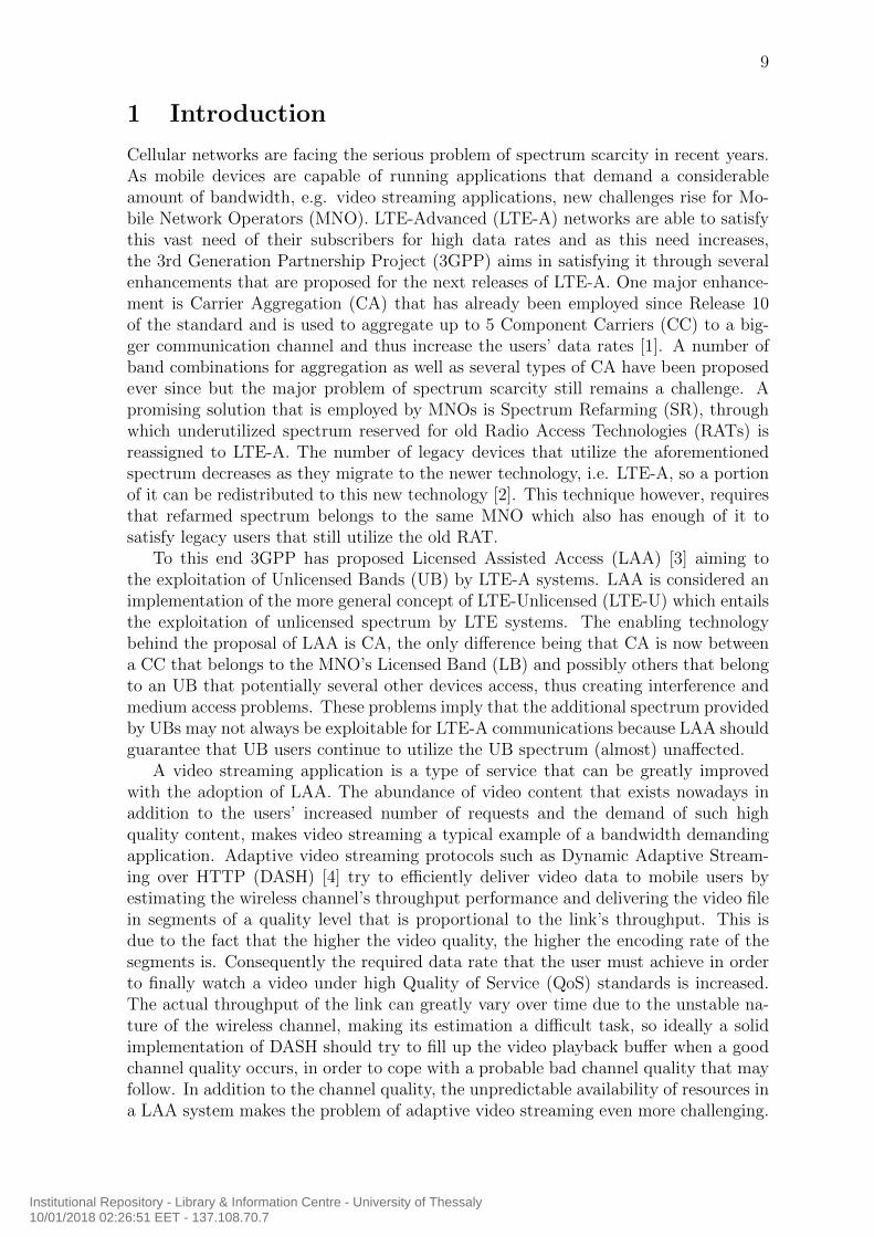
Cellular networks are facing the serious problem of spectrum scarcity in recent years.As mobile devices are capable of running applications that demand a considerableamount of bandwidth, e.g. video streaming applications, new challenges rise for Mo-bile Network Operators (MNO). LTE-Advanced (LTE-A) networks are able to satisfythis vast need of their subscribers for high data rates and as this need increases,the 3rd Generation Partnership Project (3GPP) aims in satisfying it through severalenhancements that are proposed for the next releases of LTE-A. One major enhance-ment is Carrier Aggregation (CA) that has already been employed since Release 10of the standard and is used to aggregate up to 5 Component Carriers (CC) to a big-ger communication channel and thus increase the users’ data rates [1]. A number ofband combinations for aggregation as well as several types of CA have been proposedever since but the major problem of spectrum scarcity still remains a challenge. Apromising solution that is employed by MNOs is Spectrum Refarming (SR), throughwhich underutilized spectrum reserved for old Radio Access Technologies (RATs) isreassigned to LTE-A. The number of legacy devices that utilize the aforementionedspectrum decreases as they migrate to the newer technology, i.e. LTE-A, so a portionof it can be redistributed to this new technology [2]. This technique however, requiresthat refarmed spectrum belongs to the same MNO which also has enough of it tosatisfy legacy users that still utilize the old RAT.

To this end 3GPP has proposed Licensed Assisted Access (LAA) [3] aiming tothe exploitation of Unlicensed Bands (UB) by LTE-A systems. LAA is considered animplementation of the more general concept of LTE-Unlicensed (LTE-U) which entailsthe exploitation of unlicensed spectrum by LTE systems. The enabling technologybehind the proposal of LAA is CA, the only difference being that CA is now betweena CC that belongs to the MNO’s Licensed Band (LB) and possibly others that belongto an UB that potentially several other devices access, thus creating interference andmedium access problems. These problems imply that the additional spectrum providedby UBs may not always be exploitable for LTE-A communications because LAA shouldguarantee that UB users continue to utilize the UB spectrum (almost) unaffected.

A video streaming application is a type of service that can be greatly improvedwith the adoption of LAA. The abundance of video content that exists nowadays inaddition to the users’ increased number of requests and the demand of such highquality content, makes video streaming a typical example of a bandwidth demandingapplication. Adaptive video streaming protocols such as Dynamic Adaptive Stream-ing over HTTP (DASH) [4] try to efficiently deliver video data to mobile users byestimating the wireless channel’s throughput performance and delivering the video filein segments of a quality level that is proportional to the link’s throughput. This isdue to the fact that the higher the video quality, the higher the encoding rate of thesegments is. Consequently the required data rate that the user must achieve in orderto finally watch a video under high Quality of Service (QoS) standards is increased.The actual throughput of the link can greatly vary over time due to the unstable na-ture of the wireless channel, making its estimation a difficult task, so ideally a solidimplementation of DASH should try to fill up the video playback buffer when a goodchannel quality occurs, in order to cope with a probable bad channel quality that mayfollow. In addition to the channel quality, the unpredictable availability of resources ina LAA system makes the problem of adaptive video streaming even more challenging.

Institutional Repository - Library & Information Centre - University of Thessaly10/01/2018 02:26:51 EET - 137.108.70.7

10

RBRB

Frequency

Timeslot

subframe

12 sub-carriers

7 OFDM symbols

Resource Element

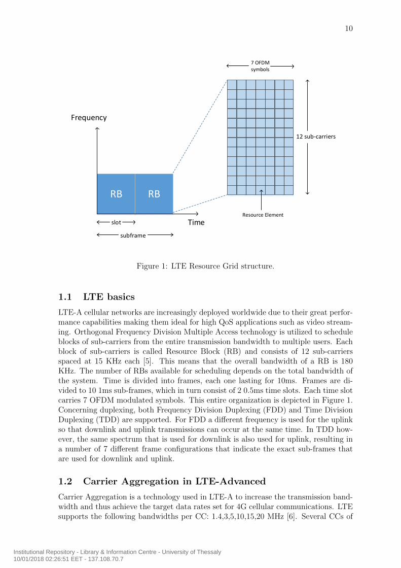
Figure 1: LTE Resource Grid structure.

1.1 LTE basics

LTE-A cellular networks are increasingly deployed worldwide due to their great perfor-mance capabilities making them ideal for high QoS applications such as video stream-ing. Orthogonal Frequency Division Multiple Access technology is utilized to scheduleblocks of sub-carriers from the entire transmission bandwidth to multiple users. Eachblock of sub-carriers is called Resource Block (RB) and consists of 12 sub-carriersspaced at 15 KHz each [5]. This means that the overall bandwidth of a RB is 180KHz. The number of RBs available for scheduling depends on the total bandwidth ofthe system. Time is divided into frames, each one lasting for 10ms. Frames are di-vided to 10 1ms sub-frames, which in turn consist of 2 0.5ms time slots. Each time slotcarries 7 OFDM modulated symbols. This entire organization is depicted in Figure 1.Concerning duplexing, both Frequency Division Duplexing (FDD) and Time DivisionDuplexing (TDD) are supported. For FDD a different frequency is used for the uplinkso that downlink and uplink transmissions can occur at the same time. In TDD how-ever, the same spectrum that is used for downlink is also used for uplink, resulting ina number of 7 different frame configurations that indicate the exact sub-frames thatare used for downlink and uplink.

1.2 Carrier Aggregation in LTE-Advanced

Carrier Aggregation is a technology used in LTE-A to increase the transmission band-width and thus achieve the target data rates set for 4G cellular communications. LTEsupports the following bandwidths per CC: 1.4,3,5,10,15,20 MHz [6]. Several CCs of

Institutional Repository - Library & Information Centre - University of Thessaly10/01/2018 02:26:51 EET - 137.108.70.7

11

LTE-A eNodeB

LTE-A UE

Band 1

Band 1

Band 1 Band 2

Intra-band, contiguous

Intra-band, non-contiguous

Inter-band, non-contiguous

Figure 2: Types of Carrier Aggregation.

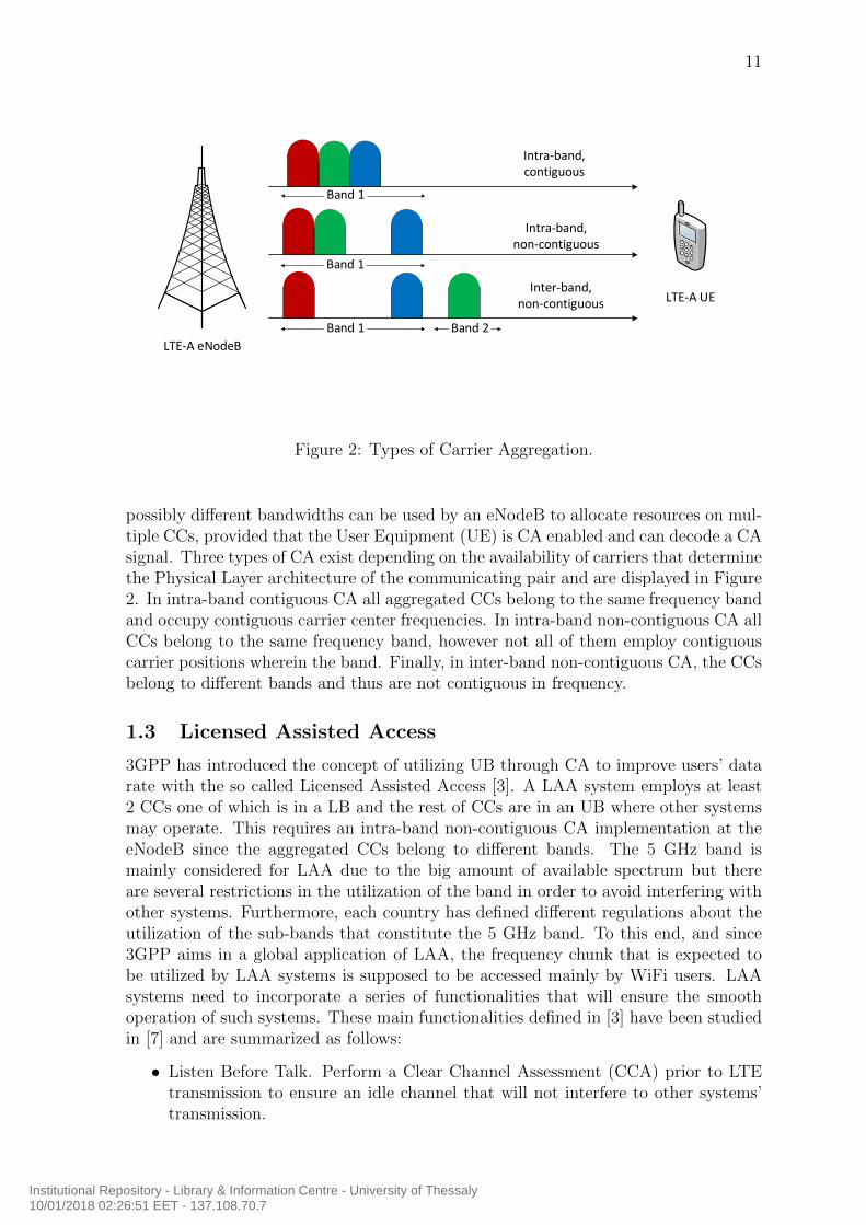
possibly different bandwidths can be used by an eNodeB to allocate resources on mul-tiple CCs, provided that the User Equipment (UE) is CA enabled and can decode a CAsignal. Three types of CA exist depending on the availability of carriers that determinethe Physical Layer architecture of the communicating pair and are displayed in Figure2. In intra-band contiguous CA all aggregated CCs belong to the same frequency bandand occupy contiguous carrier center frequencies. In intra-band non-contiguous CA allCCs belong to the same frequency band, however not all of them employ contiguouscarrier positions wherein the band. Finally, in inter-band non-contiguous CA, the CCsbelong to different bands and thus are not contiguous in frequency.

1.3 Licensed Assisted Access

3GPP has introduced the concept of utilizing UB through CA to improve users’ datarate with the so called Licensed Assisted Access [3]. A LAA system employs at least2 CCs one of which is in a LB and the rest of CCs are in an UB where other systemsmay operate. This requires an intra-band non-contiguous CA implementation at theeNodeB since the aggregated CCs belong to different bands. The 5 GHz band ismainly considered for LAA due to the big amount of available spectrum but thereare several restrictions in the utilization of the band in order to avoid interfering withother systems. Furthermore, each country has defined different regulations about theutilization of the sub-bands that constitute the 5 GHz band. To this end, and since3GPP aims in a global application of LAA, the frequency chunk that is expected tobe utilized by LAA systems is supposed to be accessed mainly by WiFi users. LAAsystems need to incorporate a series of functionalities that will ensure the smoothoperation of such systems. These main functionalities defined in [3] have been studiedin [7] and are summarized as follows:

• Listen Before Talk. Perform a Clear Channel Assessment (CCA) prior to LTEtransmission to ensure an idle channel that will not interfere to other systems’transmission.

Institutional Repository - Library & Information Centre - University of Thessaly10/01/2018 02:26:51 EET - 137.108.70.7

12

• Carrier Selection. The aggregated CC in the UB should be on a low traf-fic/interference condition concerning the activity of other systems.

• Discontinuous Transmission. LAA transmissions cannot occupy the UB indefi-nitely, and give the chance to other systems that compete for the same channelto transmit their data.

• Transmit Power Control. Regulations in different regions of the world impose amaximum transmit power level in unlicensed bands.

It is clear that all the above functionalities and their implementation puts theavailability of UB spectrum under question. A LAA system may schedule its usersin multiple CCs through CA but whether the UB CC will be available or not, highlydepends on other systems’ activity and implementation of the aforementioned func-tionalities.

1.4 Adaptive video streaming

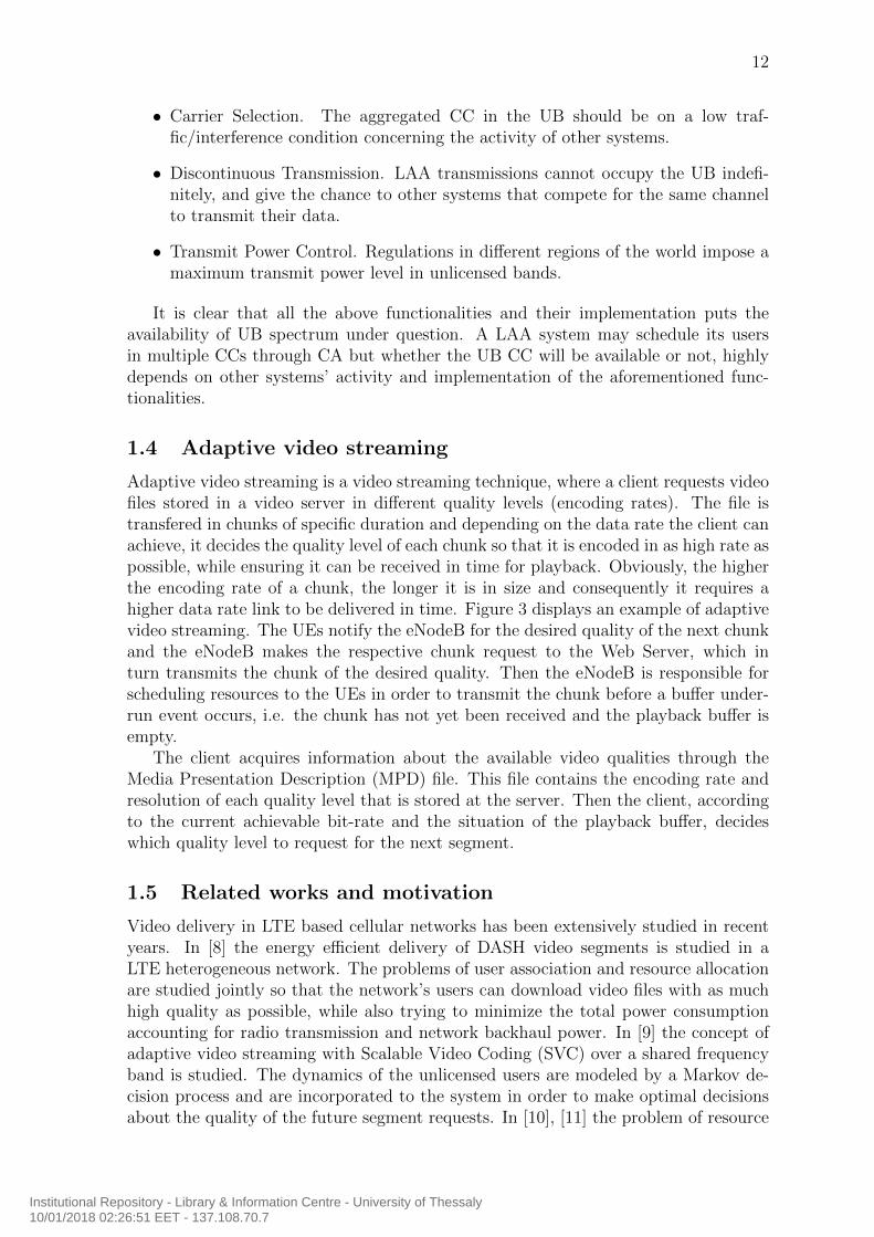
Adaptive video streaming is a video streaming technique, where a client requests videofiles stored in a video server in different quality levels (encoding rates). The file istransfered in chunks of specific duration and depending on the data rate the client canachieve, it decides the quality level of each chunk so that it is encoded in as high rate aspossible, while ensuring it can be received in time for playback. Obviously, the higherthe encoding rate of a chunk, the longer it is in size and consequently it requires ahigher data rate link to be delivered in time. Figure 3 displays an example of adaptivevideo streaming. The UEs notify the eNodeB for the desired quality of the next chunkand the eNodeB makes the respective chunk request to the Web Server, which inturn transmits the chunk of the desired quality. Then the eNodeB is responsible forscheduling resources to the UEs in order to transmit the chunk before a buffer under-run event occurs, i.e. the chunk has not yet been received and the playback buffer isempty.

The client acquires information about the available video qualities through theMedia Presentation Description (MPD) file. This file contains the encoding rate andresolution of each quality level that is stored at the server. Then the client, accordingto the current achievable bit-rate and the situation of the playback buffer, decideswhich quality level to request for the next segment.

1.5 Related works and motivation

Video delivery in LTE based cellular networks has been extensively studied in recentyears. In [8] the energy efficient delivery of DASH video segments is studied in aLTE heterogeneous network. The problems of user association and resource allocationare studied jointly so that the network’s users can download video files with as muchhigh quality as possible, while also trying to minimize the total power consumptionaccounting for radio transmission and network backhaul power. In [9] the concept ofadaptive video streaming with Scalable Video Coding (SVC) over a shared frequencyband is studied. The dynamics of the unlicensed users are modeled by a Markov de-cision process and are incorporated to the system in order to make optimal decisionsabout the quality of the future segment requests. In [10], [11] the problem of resource

Institutional Repository - Library & Information Centre - University of Thessaly10/01/2018 02:26:51 EET - 137.108.70.7

13

eNodeB

Encoder

High Quality

Low Quality

Video Input

Video Server

Figure 3: Adaptive video streaming illustration.

allocation in LTE CA systems is considered. The solution involves rate allocation ofmultiple CCs to the UEs of the network by maximizing logarithmic and sigmoidal likeutility functions that represent user satisfaction. In addition, a distributed versionof the resource allocation algorithm is presented, that is based on UE bidding for re-sources process. In [12] a scheduling framework (AVIS) for adaptive video streamingover cellular networks is presented. The authors propose a gateway level architecturefor AVIS by implementing it in two entities. The first one is responsible for decidingthe encoding rate for each user, while the second one allocates resources in a way thatthe users’ average data rate is kept stable so that segments are downloaded on time.While this framework is in many ways similar to the one proposed in this work, itlacks exploitation of UE buffer status as well as unlicensed band availability infor-mation. In [13] resource allocation is achieved by an interference mitigation schemefor Heterogeneous Networks. A stochastic scheduling algorithm is applied to scheduleresources probabilistically, that is also observed to increase femtocell capacity. Theworks in [14], [15] study admission/congestion control and transmission scheduling insmall cell networks for adaptive video streaming. More specifically in [14], a networkutility maximization problem is formulated in order to keep transmission queues ofhelper nodes stable. The admission control policy problem is tackled by choosingthe helper node as the one with the smallest queue backlog. Transmission schedulingrequires the maximization of sum rates with the queue backlogs serving as weights.Furthermore in [15], an algorithm is proposed that calculates the pre-buffering andre-buffering time for each user so that they can experience a smooth streaming servicewithout buffer under-run events. A similar work is also presented in [16], where usersare able to download from a number of base stations and decide which of them isbetter to serve them.

The main contribution of this work is that it combines the adaptive video stream-ing framework of DASH with opportunistic scheduling due to the existence of theunlicensed CC under the LAA concept. Although adaptive video streaming frame-works have been extensively studied before, there is no work studying the applicationof adaptive video streaming over a LAA system. Furthermore, since LAA is key forfuture 5G networks, the increased data rate performance it can offer is extremely im-portant for applications that require high data rates such as video streaming, thusmotivating this work.

Institutional Repository - Library & Information Centre - University of Thessaly10/01/2018 02:26:51 EET - 137.108.70.7

14

2 System model

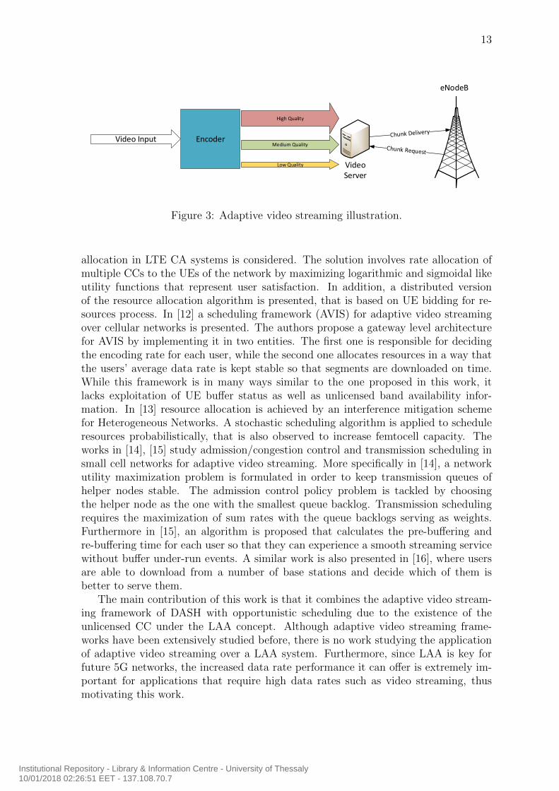
We consider a LTE-A eNodeB with LAA capabilities, i.e. the functionalities describedin Section 1.3, enabling it to monitor traffic in one or more unlicensed band CCs. Ateach scheduling interval t, the eNodeB can employ CA to schedule resources from alicensed primary CC and an unlicensed secondary CC, both in FDD mode, each oneof bandwidth WL and WU respectively. Depending on the values of WL and WU anumber of RBs ML and MU are available for scheduling. Each RB consists of 12 sub-carriers spaced at 15 KHz providing a total bandwidth of W = 180 KHz per RB. Aset of UEs K exists in the area of the eNodeB and each user k ∈ K requests DASHvideo files. A visual representation of the system is depicted in Figure 4. UEs are inthe coverage area of the licensed carrier (light blue color) and the unlicensed one (darkblue color), where WiFi systems also operate. The coverage area of the unlicensedcarrier is typically smaller because it is centered at a higher frequency.

eNodeB

UE

WiFi Access Point

WiFi user

Figure 4: The considered network topology.

2.1 Video streaming

The encoding rate of each video chunk is typically decided by the UE approximatelyevery 10 seconds (each chunk no matter its size corresponds to 10 seconds video dura-tion). We denote this time period as the Quality Selection Interval (QSI). The eNodeBdecides the quality for each UE depending on channel quality, secondary CC availabil-ity and buffer status of the UEs. Since the QSI is relatively long, it is reasonable toassume that each UE can communicate all necessary information such as buffer status

Institutional Repository - Library & Information Centre - University of Thessaly10/01/2018 02:26:51 EET - 137.108.70.7

15

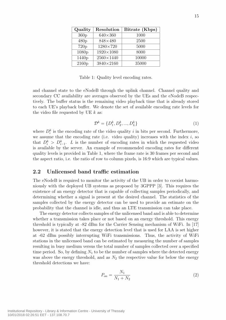
Quality Resolution Bitrate (Kbps)360p 640×360 1000480p 848×480 2500720p 1280×720 50001080p 1920×1080 80001440p 2560×1440 100002160p 3840×2160 35000

Table 1: Quality level encoding rates.

and channel state to the eNodeB through the uplink channel. Channel quality andsecondary CC availability are averages observed by the UEs and the eNodeB respec-tively. The buffer status is the remaining video playback time that is already storedto each UE’s playback buffer. We denote the set of available encoding rate levels forthe video file requested by UE k as:

Dk = {Dk1 , D

k2 , ..., D

kL} (1)

where Dki is the encoding rate of the video quality i in bits per second. Furthermore,

we assume that the encoding rate (i.e. video quality) increases with the index i, sothat Dk

i > Dki−1. L is the number of encoding rates in which the requested video

is available by the server. An example of recommended encoding rates for differentquality levels is provided in Table 1, where the frame rate is 30 frames per second andthe aspect ratio, i.e. the ratio of row to column pixels, is 16:9 which are typical values.

2.2 Unlicensed band traffic estimation

The eNodeB is required to monitor the activity of the UB in order to coexist harmo-niously with the deployed UB systems as proposed by 3GPPP [3]. This requires theexistence of an energy detector that is capable of collecting samples periodically, anddetermining whether a signal is present at the desired channel. The statistics of thesamples collected by the energy detector can be used to provide an estimate on theprobability that the channel is idle, and thus an LTE transmission can take place.

The energy detector collects samples of the unlicensed band and is able to determinewhether a transmission takes place or not based on an energy threshold. This energythreshold is typically at -82 dBm for the Carrier Sensing mechanism of WiFi. In [17]however, it is stated that the energy detection level that is used for LAA is set higherat -62 dBm possibly interrupting WiFi transmissions. Thus, the activity of WiFistations in the unlicensed band can be estimated by measuring the number of samplesresulting in busy medium versus the total number of samples collected over a specifiedtime period. So, by defining N1 to be the number of samples where the detected energywas above the energy threshold, and as N2 the respective value for below the energythreshold detections we have:

Pon =N1

N1 +N2

(2)

Institutional Repository - Library & Information Centre - University of Thessaly10/01/2018 02:26:51 EET - 137.108.70.7

16

being the probability that the unlicensed band is occupied and

Poff =N2

N1 +N2

(3)

the probability that the unlicensed band is idle at some random time instance.The works of Bianchi [18], [19] provide a solid mathematical framework for mod-

eling WiFi users’ channel access probability using a discrete time Markov chain areconsidered, in order to calculate Poff under several realistic scenarios. Particularlyin [19], the probability that a WiFi station transmits at a random slot is given as:

γ =2(1− 2p)

(1− 2p)(Win+ 1) + pWin(1− (2p)i)(4)

where Win is the minimum backoff window of 802.11 Distributed Coordination Func-tion (DCF), p is the probability that a transmitted packet collides and i is the maxi-mum number of times the backoff window is doubled after consecutive packet collisions.Assuming a number of n stations want to transmit a packet during a slot, p is givenby:

p = 1− (1− γ)n−1 (5)

since at least one of the remaining n−1 stations should also transmit so that a collisionoccurs. By solving (4) and (5) we obtain the values of γ and p and the probability ptxthat during a random WiFi slot there is at least one transmission that can be detectedby the LAA eNodeB (perfect detection is assumed) is given by :

ptx = 1− (1− γ)n (6)

We define Ψ to be the random variable that represents the number of consecutiveidle slots between two WiFi transmissions. Then the mean of Ψ is given by:

E{Ψ} =1

ptx− 1 (7)

where E{·} denotes the expectation of a random variable. One more thing is requiredfor the calculation of Poff . That is the average duration of a packet transmission inWiFi slots, since E{Ψ} is also calculated in WiFi slots. Assuming that this value isknown as E{P} then Poff is calculated as:

Poff =E{Ψ}

E{Ψ}+ E{P}(8)

Poff is therefore a function of Win, i, n and E{P}. From these parameters onlyn and E{P} are considered to vary during time and can affect the performance of ourLAA system. Of course these values are unknown to the eNodeB which in practice willperform energy detection based on (3). This model however is required to simulaterealistic WiFi traffic scenarios for the system’s performance analysis that will follow.

2.3 Solution approach

After quality selection decisions are made, resource allocation is handled by the eNodeBevery 10 milliseconds, i.e. the duration of one LTE frame. RBs are scheduled to the

Institutional Repository - Library & Information Centre - University of Thessaly10/01/2018 02:26:51 EET - 137.108.70.7

17

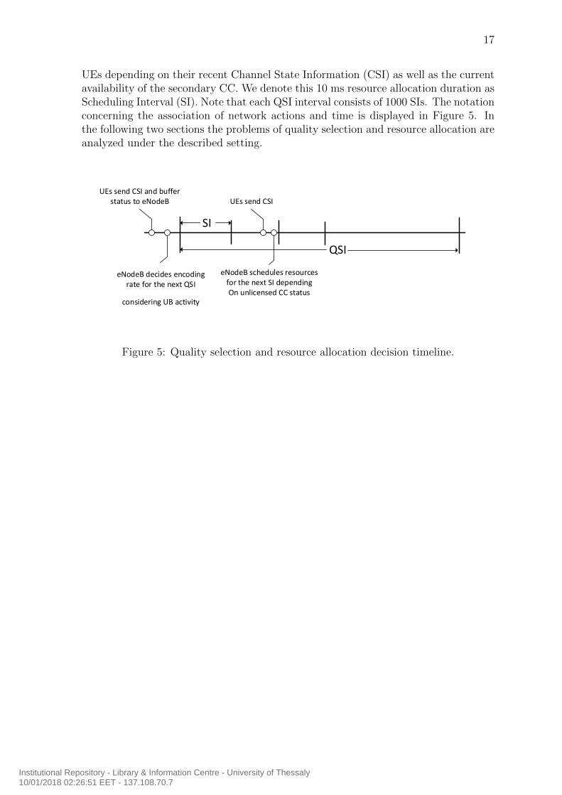
UEs depending on their recent Channel State Information (CSI) as well as the currentavailability of the secondary CC. We denote this 10 ms resource allocation duration asScheduling Interval (SI). Note that each QSI interval consists of 1000 SIs. The notationconcerning the association of network actions and time is displayed in Figure 5. Inthe following two sections the problems of quality selection and resource allocation areanalyzed under the described setting.

SI

QSI

UEs send CSI and buffer status to eNodeB

eNodeB decides encoding rate for the next QSI

considering UB activity

UEs send CSI

eNodeB schedules resourcesfor the next SI dependingOn unlicensed CC status

15-Nov-15

Figure 5: Quality selection and resource allocation decision timeline.

Institutional Repository - Library & Information Centre - University of Thessaly10/01/2018 02:26:51 EET - 137.108.70.7

18

3 Quality Selection

In order for the eNodeB to decide the video quality of the chunks to be delivered for thenext QSI, assuming that the current QSI is T , the following information is required.Each UE k ∈ K reports their average Signal to Noise Ratio (SNR) experienced ofQSI T . These values are denoted by SNRk

L(T ) and SNRkU(T ) for the licensed and

unlicensed CCs respectively. In addition, the UEs should provide their playback bufferstatus.

3.1 Buffer dynamics modeling

For the UE buffer we assume that during each QSI T , the downloading of the segmentto be displayed during the next QSI T + 1 occurs. The duration of buffered video atQSI T for UE k is given by Bk(T ) and is updated for the next QSI as:

Bk(T + 1) =

Sk(T )Rk(T )

, if Bk(T ) = 10

Bk(T ) + Sk(T )Rk(T )

, if Bk(T ) + Sk(T )Rk(T )

< 10

Bk(T ) + Sk(T )Rk(T )

− 10, if Bk(T ) + Sk(T )Rk(T )

≥ 10

(9)

where Bk(T ) is the video duration in seconds stored at QSI T and Sk(T )Rk(T )

is the

video duration downloaded at QSI T . Sk(T ) denotes the size of the segment(s) in bitsto be delivered during QSI T , while Rk(T ) denotes the average download rate duringQSI T . Differentiating from the work in [20], we assume that at the beginning of eachQSI T , the buffer empties by the amount of 10 seconds if the video segment of theprevious QSI T −1 has been downloaded. If that is not the case, the buffer occupancy

at the beginning of QSI T is Sk(T )Rk(T )

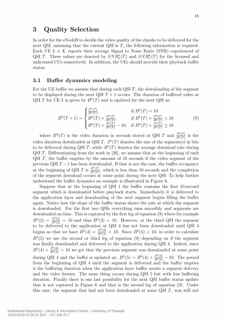
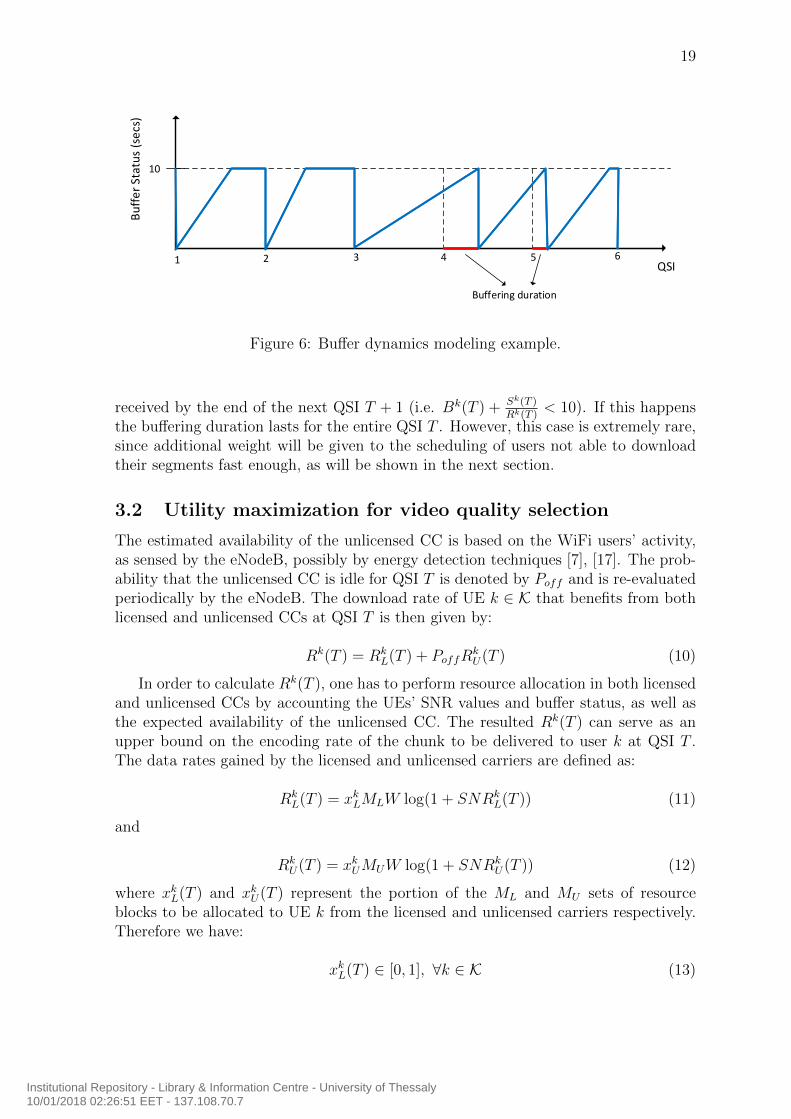
, which is less than 10 seconds and the completionof the segment download occurs at some point during the next QSI. To help furtherunderstand the buffer dynamics an example is illustrated in Figure 6.

Suppose that at the beginning of QSI 1 the buffer contains the first 10-secondsegment which is downloaded before playback starts. Immediately it is delivered tothe application layer and downloading of the next segment begins filling the bufferagain. Notice how the slope of the buffer status shows the rate at which the segmentis downloaded. For the first two QSIs everything runs smoothly and segments aredownloaded on time. This is captured by the first leg of equation (9) where for example

Bk(2) = Sk(2)Rk(2)

= 10 and thus Bk(3) = 10. However, at the third QSI the segmentto be delivered to the application at QSI 4 has not been downloaded until QSI 4

begins so that we have Bk(4) = Sk(3)Rk(3)

< 10. Since Bk(4) < 10, in order to calculate

Bk(5) we use the second or third leg of equation (9) depending on if the segmentwas finally downloaded and delivered to the application during QSI 4. Indeed, since

Bk(4) + Sk(4)Rk(4)

> 10 we get that the previous segment was downloaded at some point

during QSI 4 and the buffer is updated as: Bk(5) = Bk(4) + Sk(4)Rk(4)

− 10. The periodfrom the beginning of QSI 4 until the segment is delivered and the buffer emptiesis the buffering duration when the application layer buffer awaits a segment deliveryand the video freezes. The same thing occurs during QSI 5 but with less bufferingduration. Finally there is one last possibility for the next QSI buffer status updatethat is not captured in Figure 6 and that is the second leg of equation (9). Underthis case, the segment that had not been downloaded at some QSI T , was still not

Institutional Repository - Library & Information Centre - University of Thessaly10/01/2018 02:26:51 EET - 137.108.70.7

19

QSI

Bu

ffe

r St

atu

s (s

ecs

)

10

1 2 3 4 5 6

Buffering duration

Figure 6: Buffer dynamics modeling example.

received by the end of the next QSI T + 1 (i.e. Bk(T ) + Sk(T )Rk(T )

< 10). If this happensthe buffering duration lasts for the entire QSI T . However, this case is extremely rare,since additional weight will be given to the scheduling of users not able to downloadtheir segments fast enough, as will be shown in the next section.

3.2 Utility maximization for video quality selection

The estimated availability of the unlicensed CC is based on the WiFi users’ activity,as sensed by the eNodeB, possibly by energy detection techniques [7], [17]. The prob-ability that the unlicensed CC is idle for QSI T is denoted by Poff and is re-evaluatedperiodically by the eNodeB. The download rate of UE k ∈ K that benefits from bothlicensed and unlicensed CCs at QSI T is then given by:

Rk(T ) = RkL(T ) + PoffR

kU(T ) (10)

In order to calculate Rk(T ), one has to perform resource allocation in both licensedand unlicensed CCs by accounting the UEs’ SNR values and buffer status, as well asthe expected availability of the unlicensed CC. The resulted Rk(T ) can serve as anupper bound on the encoding rate of the chunk to be delivered to user k at QSI T .The data rates gained by the licensed and unlicensed carriers are defined as:

RkL(T ) = xkLMLW log(1 + SNRk

L(T )) (11)

and

RkU(T ) = xkUMUW log(1 + SNRk

U(T )) (12)

where xkL(T ) and xkU(T ) represent the portion of the ML and MU sets of resourceblocks to be allocated to UE k from the licensed and unlicensed carriers respectively.Therefore we have:

xkL(T ) ∈ [0, 1], ∀k ∈ K (13)

Institutional Repository - Library & Information Centre - University of Thessaly10/01/2018 02:26:51 EET - 137.108.70.7

20

and

xkU(T ) ∈ [0, 1], ∀k ∈ K (14)

Thus, we can define a utility function for each UE k based on Rk(T ) and Bk(T ),in order to decide the resource allocation that will provide a certain quality selectiondecision for QSI T as follows:

Uk(T ) = log(Rk(T ) + αBk(T )) (15)

where α is a biasing factor that will affect the impact of the UEs’ buffer status onresource allocation and therefore on quality selection decisions. Notice how the bufferstatus affects rate allocation. Due to the logarithmic function, UEs with smallerbuffer status will tend to be allocated more resources towards balancing their bufferstatus and will thus manage to download their segment on time. Equation (15) is aconcave function with respect to xkL(T ) and xkU(T ) so we can formulate the sum utilitymaximization problem P1 defined as:

P1 : maxxL,xU

∑k∈K

Uk(T ) (16)

subject to: ∑k∈K

xkL(T ) = 1 (17)

∑k∈K

xkU(T ) = 1 (18)

where xL contains variables xkL(T ), ∀k ∈ K, xU contains variables xkU(T ), ∀k ∈ K.The above problem can be solved with standard convex optimization techniques.

Let us define the augmented Lagrangian function by embedding the constraints (17)and (18) in the objective function:

L(xL,xU , λ, µ) = IkUk(T )− λ(Ikx

kL(T )− 1)− µ(Ikx

kU(T )− 1)−

ρ

2(Ikx

kL(T )− 1)2 − ρ

2(Ikx

kU(T )− 1)2

(19)

where λ, µ are Lagrangian multipliers for each of the two constraints, Ik is a unitaryrow vector of length |K| and ρ > 0.

In order to maximize L we perform the Alternating Direction Method of Multipli-ers (ADMM) [21], which involves optimizing L over each variable separately at eachiteration τ . Formally we have:

xτ+1L := arg max

xL

L(xL,xτU , λ

τ , µτ ) (20)

xτ+1U := arg max

xU

L(xτ+1L ,xU , λ

τ , µτ ) (21)

λτ+1 := λτ + ρ(Ikxτ+1L − 1) + ρ(Ikx

τ+1U − 1) (22)

Institutional Repository - Library & Information Centre - University of Thessaly10/01/2018 02:26:51 EET - 137.108.70.7

21

µτ+1 := µτ + ρ(Ikxτ+1L − 1) + ρ(Ikx

τ+1U − 1) (23)

Each of the equations (20) - (21) is solved by setting the partial derivative of L equalto zero, and solving for each variable, which is then used to obtain the Lagrangianvariables for iteration τ + 1 through (22) - (23). When ADMM converges, the optimalsolution of P1 is found and the achievable data rate of each UE can be calculated.This upper bound of data rate will determine the quality of the video segment to bedelivered to the UE as the maximum available from Dk which does not exceed theachievable data rate Rk(T ). The proposed Quality Selection Algorithm is described inAlgorithm 1.

Algorithm 1 Quality Selection

for each QSI T doRequire: SNRk

L(T ), SNRkU(T ), Bk(T ), ∀k ∈ K, Poff

Initialize x0L,x

0U , λ

0, µ0

τ ← 0repeat

Calculate xτ+1L ,xτ+1

U , λτ+1, µτ+1 by eq. (20)-(23)τ ← τ + 1

until Optimal solution foundfor each k ∈ K do

Calculate Rk(T ) by eq. (10)-(12)Dk(T )← maxDk, {Dk(T ) ≤ Rk(T )}

end forend for

The test for convergence is carried out as follows [21]. If x∗L, x∗U , λ∗ and µ∗ are theoptimal values obtained from the ADMM algorithm, the following conditions must besatisfied:

∂L(x∗L,x∗U , λ

∗, µ∗)

∂xL

= 0 (24)

∂L(x∗L,x∗U , λ

∗, µ∗)

∂xU

= 0 (25)

Ikx∗L = 1 (26)

Ikx∗U = 1 (27)

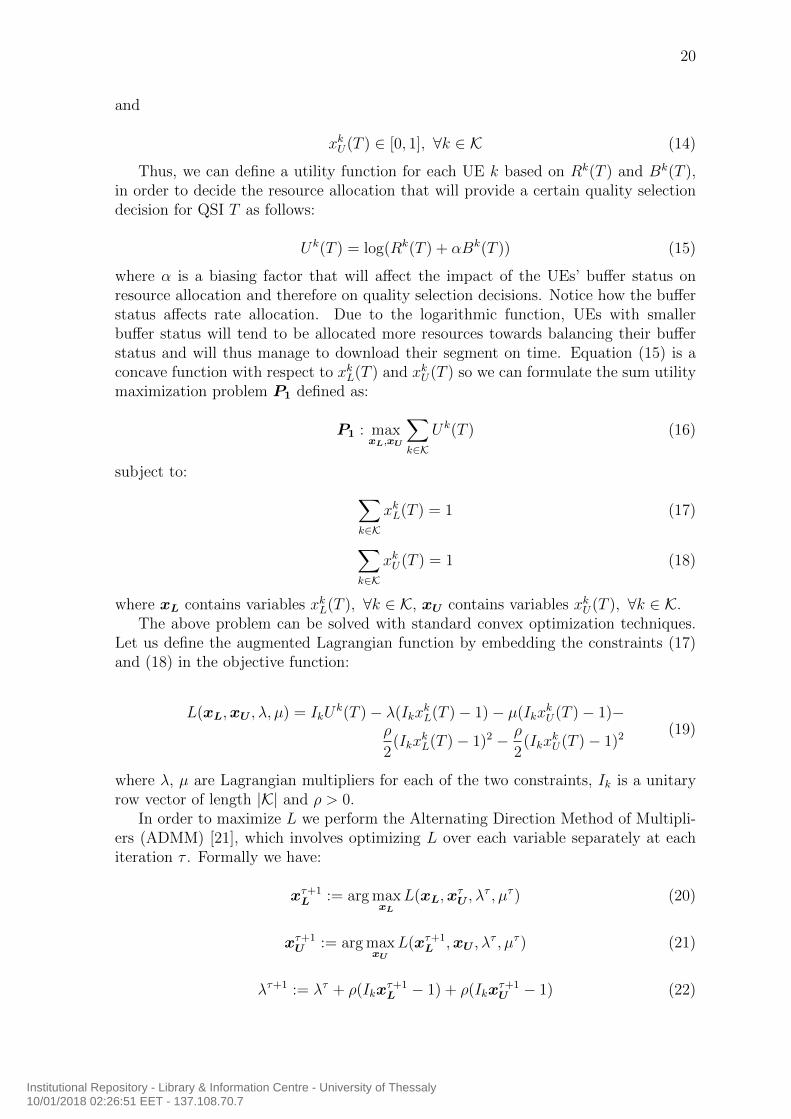
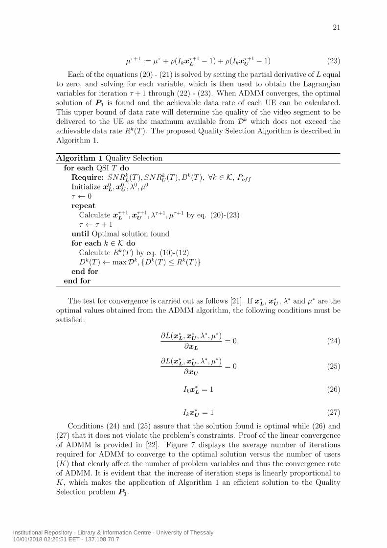
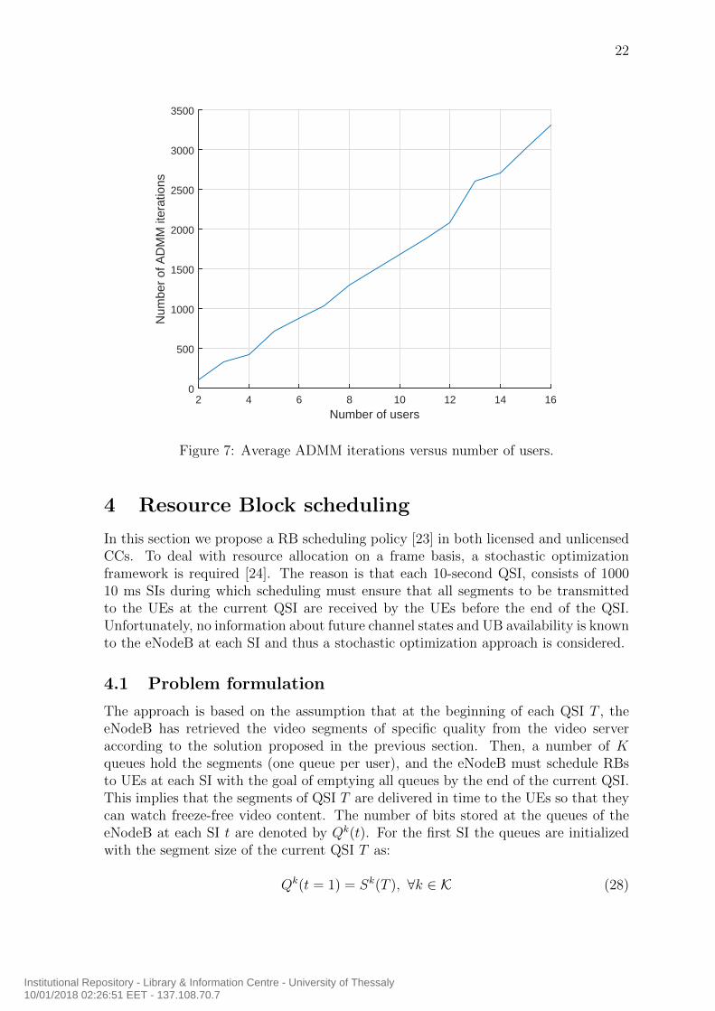
Conditions (24) and (25) assure that the solution found is optimal while (26) and(27) that it does not violate the problem’s constraints. Proof of the linear convergenceof ADMM is provided in [22]. Figure 7 displays the average number of iterationsrequired for ADMM to converge to the optimal solution versus the number of users(K) that clearly affect the number of problem variables and thus the convergence rateof ADMM. It is evident that the increase of iteration steps is linearly proportional toK, which makes the application of Algorithm 1 an efficient solution to the QualitySelection problem P1.

Institutional Repository - Library & Information Centre - University of Thessaly10/01/2018 02:26:51 EET - 137.108.70.7

22

Number of users2 4 6 8 10 12 14 16

Num

ber

of A

DM

M it

erat

ions

0

500

1000

1500

2000

2500

3000

3500

Figure 7: Average ADMM iterations versus number of users.

4 Resource Block scheduling

In this section we propose a RB scheduling policy [23] in both licensed and unlicensedCCs. To deal with resource allocation on a frame basis, a stochastic optimizationframework is required [24]. The reason is that each 10-second QSI, consists of 100010 ms SIs during which scheduling must ensure that all segments to be transmittedto the UEs at the current QSI are received by the UEs before the end of the QSI.Unfortunately, no information about future channel states and UB availability is knownto the eNodeB at each SI and thus a stochastic optimization approach is considered.

4.1 Problem formulation

The approach is based on the assumption that at the beginning of each QSI T , theeNodeB has retrieved the video segments of specific quality from the video serveraccording to the solution proposed in the previous section. Then, a number of Kqueues hold the segments (one queue per user), and the eNodeB must schedule RBsto UEs at each SI with the goal of emptying all queues by the end of the current QSI.This implies that the segments of QSI T are delivered in time to the UEs so that theycan watch freeze-free video content. The number of bits stored at the queues of theeNodeB at each SI t are denoted by Qk(t). For the first SI the queues are initializedwith the segment size of the current QSI T as:

Qk(t = 1) = Sk(T ), ∀k ∈ K (28)

Institutional Repository - Library & Information Centre - University of Thessaly10/01/2018 02:26:51 EET - 137.108.70.7

23

and are updated for the next SI by:

Qk(t+ 1) = Qk(t)− rk(t)

100, ∀k ∈ K (29)

where rk(t) is the data rate in bits per second experienced by UE k at SI t.The unlicensed carrier can either be available or unavailable at each SI according

to the UB activity as specified by LAA. The auxiliary variable au(t) indicates if theunlicensed carrier is available at SI t and thus, unlicensed carrier RBs can be allocatedat the specific SI.

au(t) =

{1, with probability Poff

0, with probability Pon(30)

The SNR experienced by each UE k ∈ K at each SI t is denoted by SNRkL(t) and

SNRkU(t) for the licensed and unlicensed band respectively. The maximum throughput

a UE can achieve at the licensed and unlicensed carriers is calculated using the currentSNR. We introduce the scheduling variable ymk(t) which is defined as:

ymk(t) =

{1, if RB m is allocated to user k

0, otherwise(31)

The data rate of UE k at each carrier is then calculated as:

rkL(t) =∑

m∈ML

ymk(t)W log(1 + SNRkL(t)) (32)

for the licensed carrier and:

rkU(t) =∑

m∈MU

ymk(t)W log(1 + SNRkU(t)) (33)

for the unlicensed carrier. The total achievable data rate of user k at SI t is thencalculated as:

rk(t) = rkL(t) + au(t)rkU(t) (34)

The goal is to schedule resources at each SI t so that by the end of the QSI T ,each UE k will have downloaded the Sk(T ) bits of the video chunk. The problem isformally expressed as:

maxymk(t)

∑k∈K

1000∑t=1

rk(t) (35)

subject to:

1000∑t=1

rk(t)

100≥ Sk(T ), ∀k ∈ K (36)

where rk(t)100

denotes the amount of bits downloaded by user k during SI t, since eachSI lasts for 10 milliseconds and rk(t) is given in bits per second.

Institutional Repository - Library & Information Centre - University of Thessaly10/01/2018 02:26:51 EET - 137.108.70.7

24

4.2 Backlog and Channel Aware Scheduling Policy

The calculation of ymk(t) ∀t ∈ [1, ..., 1000] in (35), requires prior knowledge of SNRkL(t),

SNRkU(t) and au(t) ∀t ∈ [1, ..., 1000], which is unavailable at the beginning of QSI T .

To tackle this problem we propose a scheduling policy for each SI t. It accounts for thecurrent channel conditions and unlicensed CC availability: SNRk

L(t), SNRkU(t), au(t)

as well as the users’ current backlogs Qk(t). The proposed algorithm is based on themax-weight algorithm of [24] where scheduling decisions are made based on currentqueue backlogs and channel states without the need of channel probability knowledge.

There are several scheduling policies for LTE systems in the literature [23] both fortime and frequency domain scheduling. Leveraging the Orthogonal Frequency DivisionMultiple Access (OFDMA) technology of LTE we allocate LTE RBs to different UEs ateach SI t, applying thus frequency domain scheduling. Under this type of scheduling,a metric function δ(m, k) is calculated and then each RB m is iteratively allocatedto the UE for which the metric function obtains the highest value. Proportional FairScheduling (PFS) for example, considers the users instant data rate on each RB as wellas the average rate experienced by each user in order to formulate the metric function.In our case however, each UE reports one SNR value for each CC, SNRk

L(t), SNRkU(t)

respectively. It is possible though to require sub-band instead of wide-band levelfeedback reports and thus acquire feedback in the form of SNRk

L(m, t), SNRkU(m, t),

where SNRkL(m, t) is the SNR experienced by UE k on SI t for RB m of the licensed

CC and SNRkU(m, t) is the respective value for the unlicensed CC. Whichever the case,

rk(t) can be decomposed to a series of data rates given by the different reported SNRs,whether they differ per RB or they are the same for RBs of the same CC as:

rk(t) =∑

m∈ML

ymk(t)rkL(m, t) + au(t)

∑m∈MU

ymk(t)rkU(m, t) (37)

where rkL(m, t) is given by:

rkL(m, t) = W log(1 + SNRkL(m, t)) (38)

and rkU(m, t) by:

rkU(m, t) = W log(1 + SNRkU(m, t)) (39)

which are the data rates in bits per second experienced by UE k on SI t and on RBm if m belongs to the licensed and unlicensed bands respectively. For simplicity infurther analysis we assume a wide-band feedback report system and thus equations(38) and (39) reduce to:

rkL(m, t) = W log(1 + SNRkL(t)) (40)

and

rkU(m, t) = W log(1 + SNRkU(t)) (41)

After defining the users’ instant data rate per RB we proceed by calculating theaverage throughput experienced by UE k until SI t as:

rk(t) =

∑tn=1 r

k(n)

t(42)

Institutional Repository - Library & Information Centre - University of Thessaly10/01/2018 02:26:51 EET - 137.108.70.7

25

With standard PFS [23] the metric function δ(m, k) is calculated as:

δ(m, k) =

rkL(m,t)

rk(t), if m ∈ML

rkU (m,t)

rk(t), if m ∈MU

(43)

It is evident from the form of δ(m, k) that it is maximized for UEs that experi-ence high instant data rate for RB m and low average data rate, providing thus theproportional fairness characteristic of the metric function. Equation (43) is calculatediteratively for each RB and each UE and RB m is allocated to UE k∗ that maximizesδ(m, k). Formally k∗ is given as:

k∗ = arg maxkδ(m, k), ∀m ∈ML ∪MU (44)

In our system, proportional fairness is implemented with the logarithmic functionin the objective function of the Utility maximization problem P1. At this stage,the designed scheduling policy should empty all backlog queues by the end of eachQSI. Since each QSI consists of 1000 SIs the desired scheduling policy must result in:Qk(1000) = 0, ∀k ∈ K. Driven by the results of the max-weight algorithm [24], thescheduling metric is given by the data rate experienced by each UE for the current SImultiplied (weighted) by user’s queue backlog and the scheduling decision is based onwhich UE maximizes the newly defined metric:

δ(m, k) =

{Qk(t)rkL(m, t), if m ∈ML

Qk(t)rkU(m, t), if m ∈MU

(45)

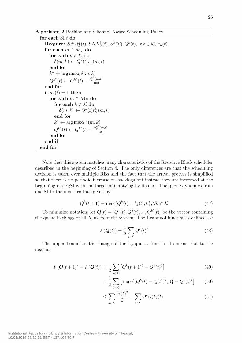
Each RB is iteratively assigned to the UE that maximizes (45). Its respective queuebacklog is updated and the procedure continues until all RBs are allocated. Next,we present the proposed Backlog and Channel Aware Scheduling Policy (BCASP) inAlgorithm 2.

4.3 BCASP analysis

For the remainder of this section we provide an insight about the conditions, underwhich the proposed BCASP manages to deliver the DASH video segments of a QSI Ton time, without the UEs experiencing any buffer under-run events which will resultin video freezes.

The max weight based BCASP algorithm utilizes the technique of Lyapunov driftminimization, which is briefly explained next. Consider a system with K queues, eachof which stores bits to be transmitted to the K users of the system. Each queue kis supplied with an arrival process that adds a number of Ak(t) bits at each SI t.The system’s scheduler must decide which user to serve at each SI t depending onthe current queue backlogs Qk(t) as well as current channel states. Suppose that thenumber of bits that can be transmitted to user k at SI t and is dependent on the

channel state is given by rk(t)100

. The number of bits that are actually transmitted touser k, depending on the scheduler’s decision is given by bk(t) which is defined as:

bk(t) =

{rk(t)100

, if k is scheduled at SI t

0, otherwise(46)

Institutional Repository - Library & Information Centre - University of Thessaly10/01/2018 02:26:51 EET - 137.108.70.7

26

Algorithm 2 Backlog and Channel Aware Scheduling Policy

for each SI t doRequire: SNRk

L(t), SNRkU(t), Sk(T ), Qk(t), ∀k ∈ K, au(t)

for each m ∈ML dofor each k ∈ K doδ(m, k)← Qk(t)rkL(m, t)

end fork∗ ← arg maxk δ(m, k)

Qk∗(t)← Qk∗(t)− rk∗

L (m,t)

100

end forif au(t) = 1 then

for each m ∈MU dofor each k ∈ K doδ(m, k)← Qk(t)rkU(m, t)

end fork∗ ← arg maxk δ(m, k)

Qk∗(t)← Qk∗(t)− rk∗

U (m,t)

100

end forend if

end for

Note that this system matches many characteristics of the Resource Block schedulerdescribed in the beginning of Section 4. The only differences are that the schedulingdecision is taken over multiple RBs and the fact that the arrival process is simplifiedso that there is no periodic increase on backlogs but instead they are increased at thebeginning of a QSI with the target of emptying by its end. The queue dynamics fromone SI to the next are thus given by:

Qk(t+ 1) = max{Qk(t)− bk(t), 0},∀k ∈ K (47)

To minimize notation, let Q(t) = [Q1(t), Q2(t), ..., QK(t)] be the vector containingthe queue backlogs of all K users of the system. The Lyapunof function is defined as:

F (Q(t)) =1

2

∑k∈K

Qk(t)2 (48)

The upper bound on the change of the Lyapunov function from one slot to thenext is:

F (Q(t+ 1))− F (Q(t)) =1

2

∑k∈K

[Qk(t+ 1)2 −Qk(t)2

](49)

=1

2

∑k∈K

[max{(Qk(t)− bk(t))2, 0} −Qk(t)2

](50)

≤∑k∈K

bk(t)2

2−∑k∈K

Qk(t)bk(t) (51)

Institutional Repository - Library & Information Centre - University of Thessaly10/01/2018 02:26:51 EET - 137.108.70.7

27

where (51) results from the fact that:

max{(A−B)2, 0} ≤ A2 +B2 − 2AB (52)

The conditional Lyapunov drift for slot t is defined as:

∆(Q(t)) = E{F (Q(t+ 1))− F (Q(t))|Q(t)

}(53)

≤ E{∑

k∈K

bk(t)2

2|Q(t)

}− E

{∑k∈K

Qk(t)bk(t)|Q(t)

}(54)

The first of the two terms in (54) is independent of Q(t) and is bounded by the valueobtained if the scheduler allocates all resources to the user with the highest rk(t) atSI t. Assuming this value is denoted as C we get:

∆(Q(t)) ≤ C − E{∑

k∈K

Qk(t)bk(t)|Q(t)

}(55)

Now, in order to minimize ∆(Q(t)), we only need to opportunistically maximize:

E{∑

k∈K

Qk(t)bk(t)|Q(t)

}(56)

which, according to the max weight algorithm in [24], is achieved by making schedul-

ing decisions that maximize Qk(t) rk(t)100

. Since scheduling decisions are taken for eachindividual RB of licensed and unlicensed CCs the scheduling metric in (45) complieswith the max weight opportunistic scheduling results.

The BCASP is designed to guarantee the stability of the transmission queues inthe long term, meaning that all video segments will be downloaded at some point, butit provides no guarantees about the short term delivery of each individual segmentduring a QSI. Channel conditions may deteriorate for all users and unlicensed carrierutilization by WiFi users may increase dramatically during a 10 second period, allowingfewer access opportunities and decreased data rates. Consequently the eNodeB mightnot be able to provide the promised data rates so that the UEs can download theirsegments on time for playback. Is there something we can do to minimize the chancesof buffer under-run events? First, the total data rate that the eNodeB must provideis mostly much lower than the one it can provide. Remember that the encodingrate of the segments to be delivered to the UEs is selected as the highest availablethat does not exceed the UE data rate calculated by equations (10)-(12) after theutility maximization problem is solved. This difference between required and availabledata rate is in most cases enough to minimize video freezes as will be shown in thenext section. In addition, a simple pre-buffering technique is proposed in [16] wherethe pre-buffering time (the time between the request of the first video segment untilplayback starts) is calculated as the maximum delay of the transmission queues of theusers. This implies that UEs can request more segments before the current segmentsare downloaded in order to get a head-start in preventing a buffer under-run eventdue to the factors already mentioned. Although such technique may even eliminatethe chances of buffer under-run events, it might also add a significant delay at thebeginning of playback which will most certainly degrade Quality of Experience (QoE)for the users.

Institutional Repository - Library & Information Centre - University of Thessaly10/01/2018 02:26:51 EET - 137.108.70.7

28

CRC Attachment

Channel Coding

Scrambling ModulationTransport Block Precoding

Layer Mapping

OFDM Modulation

Antenna

Channel Decoding

DescramblingDeprecoding

Layer Demapping

EqualizerChannel

Estimation

OFDM Demodulation

Channel

DemodulationCRC

Check

Transmitter

Receiver

Figure 8: LTE Physical Layer downlink processing chain.

5 Performance evaluation

In this section extensive simulation results on the considered LAA video streamingframework are provided. In the first two sub-sections, the simulation setup is explainedboth in link level (LTE physical layer) as well as in system level, in order to lay thefoundation for the upcoming simulations and the explanation of results in the followingsub-section.

5.1 Link level simulation setup

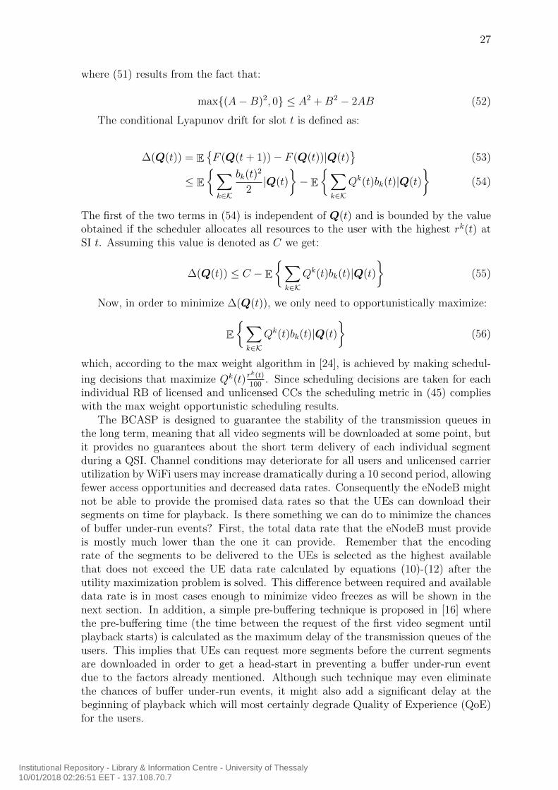
The link level simulation consists of the implementation of LTE Physical Layer inMATLAB in order to obtain performance metrics of the downlink transmission ofLTE under different channel conditions and transmission modes. The LTE downlinkprocessing chain is provided in Figure 8. The functionality of the blocks depicted inFigure 8 is briefly described as follows:

• CRC Attachment. Cyclic Redundancy Check (CRC) is used for error detectionof the transport blocks. A number of parity bits are attached to the end of thetransport block.

• Channel Coding. Turbo coding with a rate of 1/3 is usually employed to protectthe transmission of data against channel fading.

• Scrambling. The input bit streams are combined to scrambling sequences inorder to produce pseudo-random codewords.

• Modulation. The scrambled bits are used to generate complex valued modulationsymbols. The constellations supported by LTE are QPSK, 16QAM and 64QAMin order to provide adaptive modulation.

• Precoding and Layer Mapping. This functionality is employed in case of a multi-antenna transmission scheme. It involves the mapping of the input symbols oneach layer for transmission on the available antenna ports.

• OFDM Modulation. Orthogonal Frequency Division Multiplexing modulation isapplied by utilizing Inverse Fast Fourier Transform (IFFT) in order to converta frequency selective fading channel to a number of flat fading orthogonal sub-channels of narrower bandwidth.

Institutional Repository - Library & Information Centre - University of Thessaly10/01/2018 02:26:51 EET - 137.108.70.7

29

Parameter ValueBandwidth 1.4,3,5,10,15,20 MHzTx/Rx Antennas 1,2,4Modulation QPSK, 16QAM, 64QAMTx Scheme Single port, Tx Diversity, Spatial MultiplexingChannel Model EPA, EVA, ETU

Table 2: Physical layer simulation setup parameters.

The reverse actions are made at the receiver side with the addition of Channel Es-timation which is used to counteract the effects of the wireless channel on the receivedsignal and improve Bit Error Rate (BER). The procedure involves the reception ofknown pilot symbols in specific Resource Elements of the LTE Resource Grid. Thereceiver can then estimate the effect of the channel by observing the difference betweenthe known and received pilot symbols.

The simulation environment developed to model the physical layer described abovesets system parameters such as the number of frames, bandwidth, transmission schemeetc and passes the OFDM modulated signals through a fading channel for a series ofSNR values. The receiver decodes the received signals and the throughput perfor-mance of the link is calculated. A complete list of the parameters and possible valuessupported by the simulator are given in Table 2.

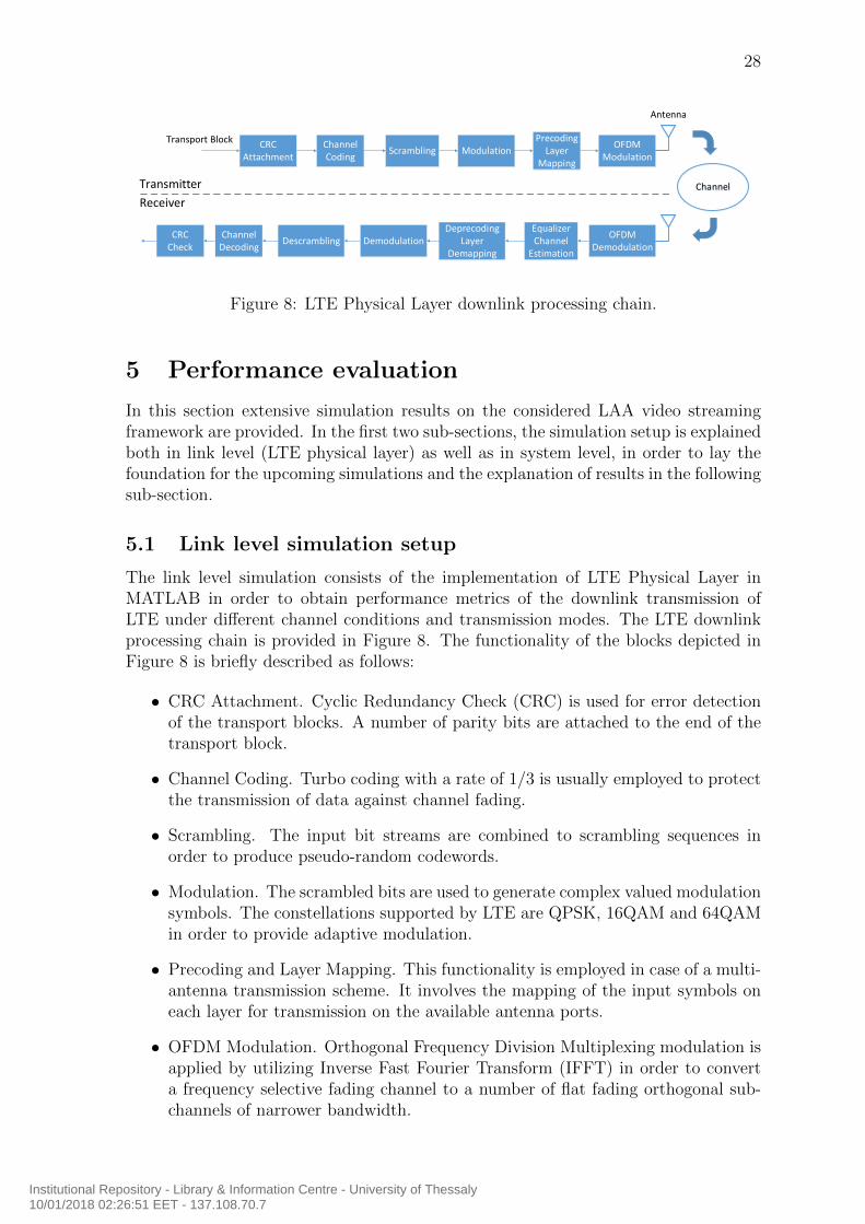
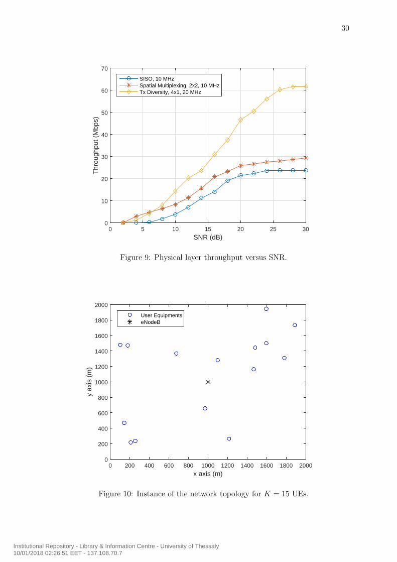
Some typical results provided by the simulator are shown in Figure 9. The durationof the simulations was 100 LTE frames and the channel model used was the ExtendedPedestrian A model. Adaptive modulation was employed according to [25]. Thefigure depicts all supported transmission schemes for different bandwidth and Tx/Rxantenna setups. In the following sections a specific setup will be used for all links inthe cellular network in order to provide system level results of the UE scheduling forvideo streaming application.

5.2 System level simulation setup

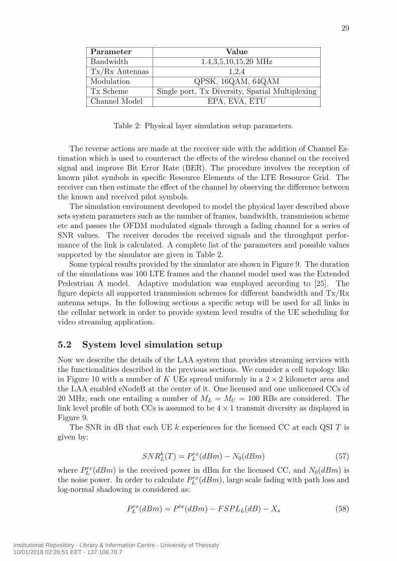
Now we describe the details of the LAA system that provides streaming services withthe functionalities described in the previous sections. We consider a cell topology likein Figure 10 with a number of K UEs spread uniformly in a 2× 2 kilometer area andthe LAA enabled eNodeB at the center of it. One licensed and one unlicensed CCs of20 MHz, each one entailing a number of ML = MU = 100 RBs are considered. Thelink level profile of both CCs is assumed to be 4× 1 transmit diversity as displayed inFigure 9.

The SNR in dB that each UE k experiences for the licensed CC at each QSI T isgiven by:

SNRkL(T ) = P rx

L (dBm)−N0(dBm) (57)

where P rxL (dBm) is the received power in dBm for the licensed CC, and N0(dBm) is

the noise power. In order to calculate P rxL (dBm), large scale fading with path loss and

log-normal shadowing is considered as:

P rxL (dBm) = P tx(dBm)− FSPLL(dB)−Xs (58)

Institutional Repository - Library & Information Centre - University of Thessaly10/01/2018 02:26:51 EET - 137.108.70.7

30

SNR (dB)0 5 10 15 20 25 30

Thr

ough

put (

Mbp

s)

0

10

20

30

40

50

60

70

SISO, 10 MHzSpatial Multiplexing, 2x2, 10 MHzTx Diversity, 4x1, 20 MHz

Figure 9: Physical layer throughput versus SNR.

x axis (m)0 200 400 600 800 1000 1200 1400 1600 1800 2000

y ax

is (

m)

0

200

400

600

800

1000

1200

1400

1600

1800

2000

User EquipmentseNodeB

Figure 10: Instance of the network topology for K = 15 UEs.

Institutional Repository - Library & Information Centre - University of Thessaly10/01/2018 02:26:51 EET - 137.108.70.7

31

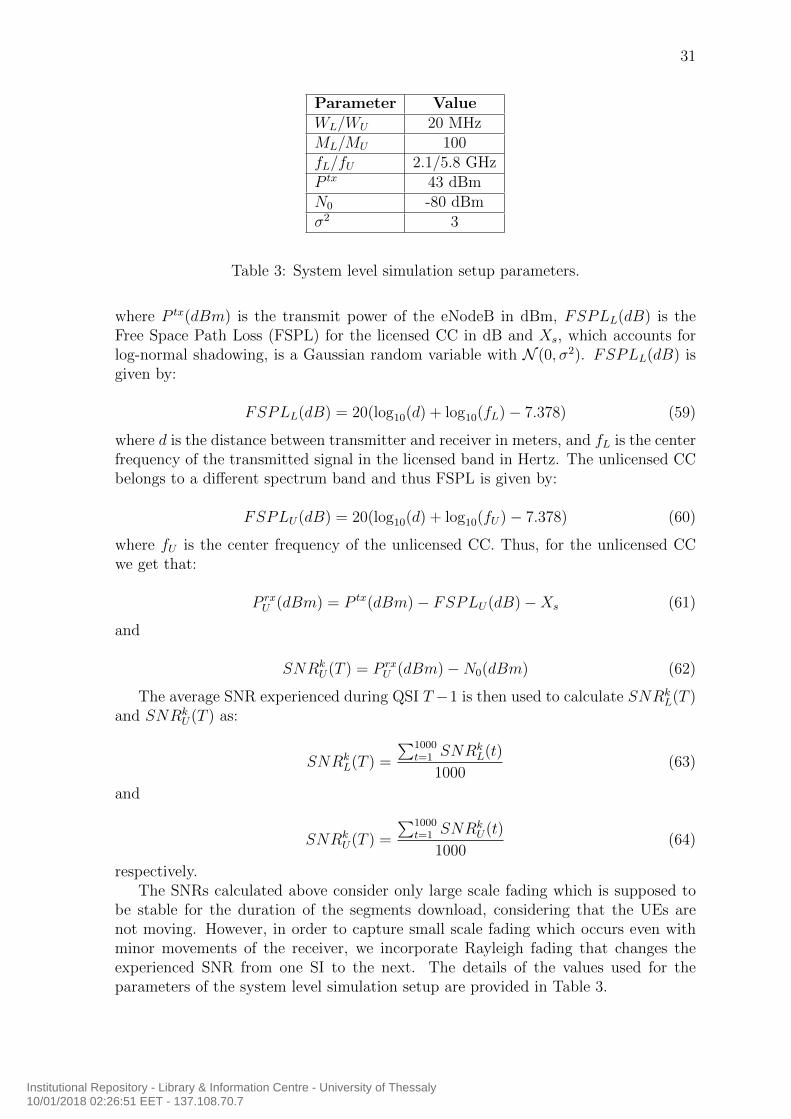
Parameter ValueWL/WU 20 MHzML/MU 100fL/fU 2.1/5.8 GHzP tx 43 dBmN0 -80 dBmσ2 3

Table 3: System level simulation setup parameters.

where P tx(dBm) is the transmit power of the eNodeB in dBm, FSPLL(dB) is theFree Space Path Loss (FSPL) for the licensed CC in dB and Xs, which accounts forlog-normal shadowing, is a Gaussian random variable with N (0, σ2). FSPLL(dB) isgiven by:

FSPLL(dB) = 20(log10(d) + log10(fL)− 7.378) (59)

where d is the distance between transmitter and receiver in meters, and fL is the centerfrequency of the transmitted signal in the licensed band in Hertz. The unlicensed CCbelongs to a different spectrum band and thus FSPL is given by:

FSPLU(dB) = 20(log10(d) + log10(fU)− 7.378) (60)

where fU is the center frequency of the unlicensed CC. Thus, for the unlicensed CCwe get that:

P rxU (dBm) = P tx(dBm)− FSPLU(dB)−Xs (61)

and

SNRkU(T ) = P rx

U (dBm)−N0(dBm) (62)

The average SNR experienced during QSI T −1 is then used to calculate SNRkL(T )

and SNRkU(T ) as:

SNRkL(T ) =

∑1000t=1 SNR

kL(t)

1000(63)

and

SNRkU(T ) =

∑1000t=1 SNR

kU(t)

1000(64)

respectively.The SNRs calculated above consider only large scale fading which is supposed to

be stable for the duration of the segments download, considering that the UEs arenot moving. However, in order to capture small scale fading which occurs even withminor movements of the receiver, we incorporate Rayleigh fading that changes theexperienced SNR from one SI to the next. The details of the values used for theparameters of the system level simulation setup are provided in Table 3.

Institutional Repository - Library & Information Centre - University of Thessaly10/01/2018 02:26:51 EET - 137.108.70.7

32

Concerning the video files that the UEs request for downloading, we consider avideo file encoded in 6 different quality levels as described in Table 1. Formally wehave that:

Dk = {1000, 2500, 5000, 8000, 10000, 35000}Kbps, ∀k ∈ K (65)

Moving on to the WiFi system setup, suppose that a random number of n WiFistations are involved in packet transmissions during each QSI. Each packet is consid-ered to have a fixed size of 1.5 KB and can be transmitted at a set of physical datarates supported by 802.11n that is operational in the 5GHz spectrum. This set Rw ofphysical WiFi data rates is as follows:

Rw = {7.2, 14.4, 21.7, 28.9, 43.3, 57.8, 65, 72.2} Mbps (66)

The rate which will be selected derives from WiFi’s rate adaptation mechanism anddepends on each station’s channel conditions. For a fixed packet size one can calculatethe transmission duration for each possible data rate and by accounting that eachWiFi slot lasts for 9 µs the set of possible transmission durations in number of WiFislots is given by:

Tw = {186, 94, 62, 47, 32, 24, 22, 19} slots (67)

Assuming that in each WiFi slot there is a number of n WiFi stations that want totransmit a packet, we can calculate Poff for each QSI by equations (4)-(8) and (67).However, since the number of competing WiFi stations during a QSI is variable, andin order to simplify WiFi operation during simulation by explicitly manipulating Poffso that its effect is evident, we assume that it follows a Gaussian distribution overQSIs as G(µ, φ2).

5.3 Simulation results

For the remainder of this section, the performance of the proposed quality selection andscheduling algorithms will be tested through indicative simulations performed usingthe setup described above. These simulations aim to highlight the effect of severalnetwork parameters such as the number of users and the unlicensed band availability,on crucial performance metrics such as average segment quality and number of videofreezes. The proposed solution that consists of Algorithms 1 and 2, both implementedon the eNodeB are compared to standard PFS and the AVIS framework [12].

With PFS, the eNodeB allocates resources according to the scheduling metric in(43). Each UE experiences an average data rate, according to which it requests theappropriate quality for the next segment using the same rule as in Algorithm 1, i.e.it requests the maximum available segment encoding rate that does not exceed theaverage experienced data rate. Since PFS is a general solution and is not specificallydesigned to address the complex problem of adaptive video streaming, the AVIS frame-work is also employed for comparison. AVIS consists of two entities. The allocator,which considers the resource requirements of the UEs and decides the encoding rate ofthe segments to be delivered to each UE, and the enforcer which allocates resourcesin a similar to PFS manner so that UEs can download the desired segments in time.This framework is very similar to the one proposed in this work with the allocator

Institutional Repository - Library & Information Centre - University of Thessaly10/01/2018 02:26:51 EET - 137.108.70.7

33

Number of users4 6 8 10 12 14

Ave

rage

Dat

a ra

te (

Mbp

s)

0

5

10

15

20

25

30

35

µ=0.2µ=0.5µ=0.8

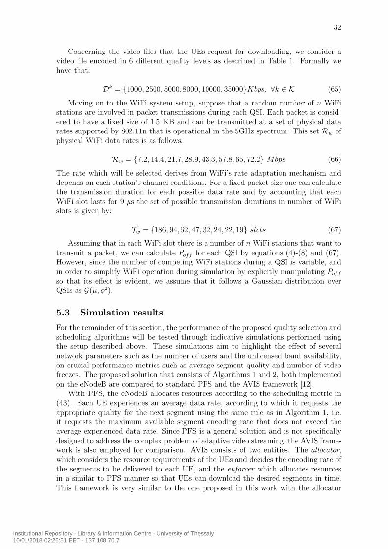
Figure 11: Average data rate vs number of UEs for different cases of unlicensed CCavailability.

matching with Algorithm 1 and the enforcer matching with Algorithm 2. Further-more, the allocator is designed to operate every 10 seconds and the enforcer every 10milliseconds which is exactly as defined in Figure 5.

5.3.1 Video Segment Quality

The chosen segment quality depends on the data rate that the network can provideto each UE. Furthermore, data rate is a function of the number of UEs associatedwith the eNodeB as well as the number of available resources which directly links tounlicensed CC availability. To highlight the impact of the above parameters on averagedata rate, Figure 11 is provided.

Unlicensed CC availability is affected by the mean value µ of Poff which varies inFigure 11 while its standard deviation remains fixed at φ2 = 0.1. As the number of UEsK increases the average data rate decreases since more UEs share the same numberof resources. The effect of unlicensed CC utilization can be seen for the three cases ofµ depicted in Figure 11. For higher values of µ the unlicensed CC access probabilityis higher, UEs can be allocated with more resources and thus enjoy higher data ratesthat can lead to better video quality and/or fewer video freezes. The increased datarate effect is stronger when the number of UEs is small and deteriorates as K increases.However, between different cases of µ the percentile drop in average data rate remainssteady. For example, the average data rate is increased by approximately 40% fromµ = 0.2 to µ = 0.8 for all values of K. This indicates that even when K is high andthe average data rate is relatively small, the increased performance due to unlicensedCC utilization is far from negligible.

Institutional Repository - Library & Information Centre - University of Thessaly10/01/2018 02:26:51 EET - 137.108.70.7

34

Segment Encoding Rate (Mbps)1 2.5 5 8 10 35

CD

F

0

0.1

0.2

0.3

0.4

0.5

0.6

0.7

0.8

0.9

1

K=3K=5K=8K=10K=12K=15

Figure 12: Segment quality CDF for different number of UEs.

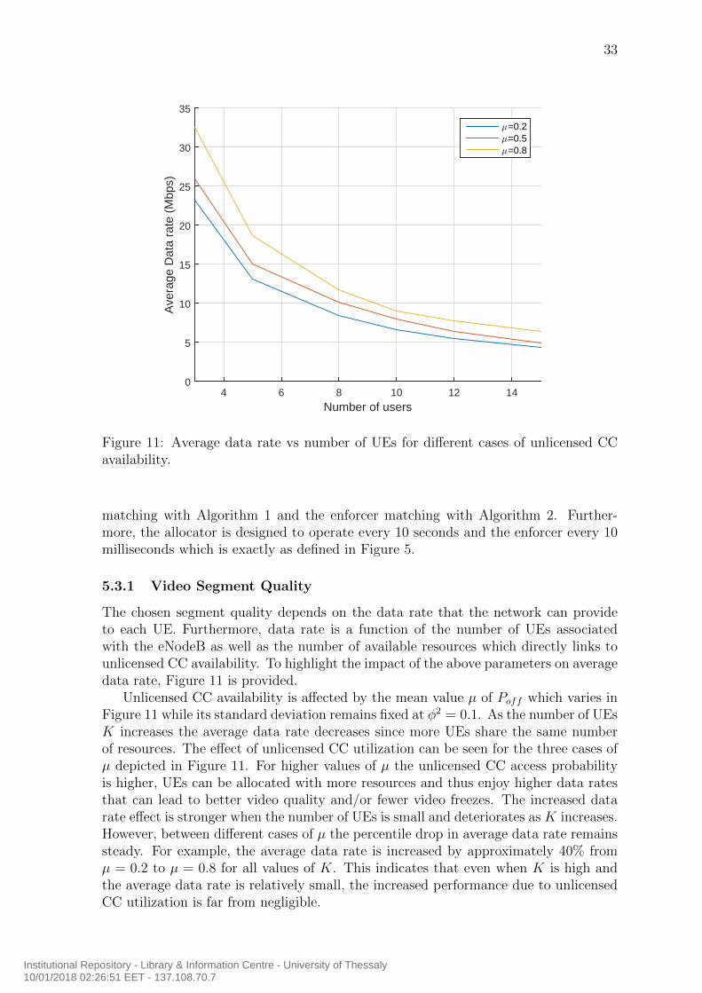
As stated before, the average segment quality mainly depends on the number ofUEs, since the more UEs are active in the network, the less resources are allocated toeach one, and thus they generally experience less throughput which leads the designedquality selection algorithm to choose lower quality segments. Figure 12 displays theCumulative Distribution Function (CDF) of the different segment qualities of (65)for several cases of number of UEs K and for a number of 100 QSIs. Probability ofunlicensed CC availability Poff is Gaussian with mean value of µ = 0.5 and standarddeviation φ2 = 0.1.

Intuition is validated through Figure 12 since CDFs for more UEs are above thosewith less UEs, meaning that they end up with more low quality segments. Morespecifically for K = 15, more than 90% of segments are delivered in the 3 lowestquality levels of 1, 2.5 and 5 Mbps and the rest of them in just 8 Mbps. On the otherhand, for K = 3, very few segments are delivered in the 4 lowest qualities, while mostof them are delivered in 10 Mbps and a small portion of under 10% is even deliveredin the highest quality of 35 Mbps.

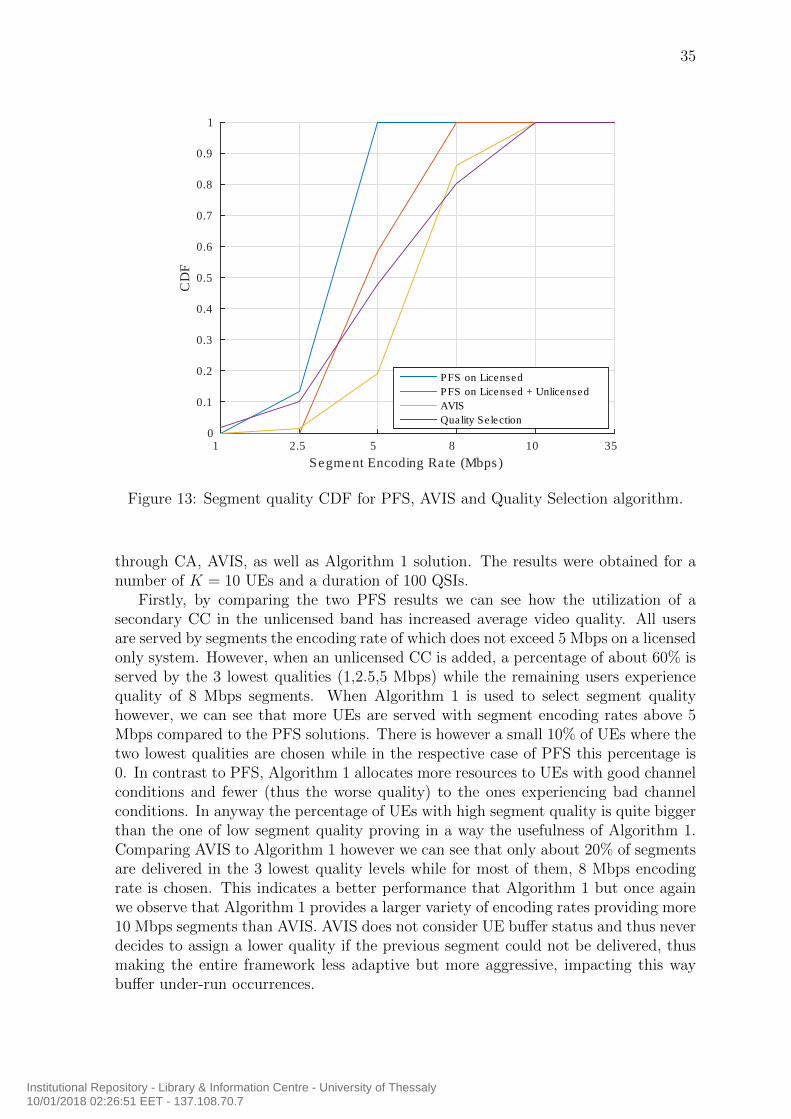
In addition to the proposed Algorithms 1 and 2 a standard PFS solution as well asthe AVIS framework are also considered for comparison. It is expected that PFS willtry to provide approximately the same QoS to all UEs and it is interesting to observethe effect of such scheduling policy on segment quality, since there is no knowledgeabout the unlicensed CC availability to the UEs that request the segments dependingon average data rate performance. On the other hand, since AVIS quality selectionis implemented on the eNodeB, there is knowledge about the number of availableresources but the scheduling is handled just like in PFS. Figure 13 displays the averagesegment quality CDF for PFS only on a licensed CC, on a licensed plus unlicensed CC

Institutional Repository - Library & Information Centre - University of Thessaly10/01/2018 02:26:51 EET - 137.108.70.7

35

Segment Encoding Rate (Mbps)

1 2.5 5 8 10 35

CD

F

0

0.1

0.2

0.3

0.4

0.5

0.6

0.7

0.8

0.9

1

PFS on Licensed

PFS on Licensed + Unlicensed

AVIS

Quality Selection

Figure 13: Segment quality CDF for PFS, AVIS and Quality Selection algorithm.

through CA, AVIS, as well as Algorithm 1 solution. The results were obtained for anumber of K = 10 UEs and a duration of 100 QSIs.

Firstly, by comparing the two PFS results we can see how the utilization of asecondary CC in the unlicensed band has increased average video quality. All usersare served by segments the encoding rate of which does not exceed 5 Mbps on a licensedonly system. However, when an unlicensed CC is added, a percentage of about 60% isserved by the 3 lowest qualities (1,2.5,5 Mbps) while the remaining users experiencequality of 8 Mbps segments. When Algorithm 1 is used to select segment qualityhowever, we can see that more UEs are served with segment encoding rates above 5Mbps compared to the PFS solutions. There is however a small 10% of UEs where thetwo lowest qualities are chosen while in the respective case of PFS this percentage is0. In contrast to PFS, Algorithm 1 allocates more resources to UEs with good channelconditions and fewer (thus the worse quality) to the ones experiencing bad channelconditions. In anyway the percentage of UEs with high segment quality is quite biggerthan the one of low segment quality proving in a way the usefulness of Algorithm 1.Comparing AVIS to Algorithm 1 however we can see that only about 20% of segmentsare delivered in the 3 lowest quality levels while for most of them, 8 Mbps encodingrate is chosen. This indicates a better performance that Algorithm 1 but once againwe observe that Algorithm 1 provides a larger variety of encoding rates providing more10 Mbps segments than AVIS. AVIS does not consider UE buffer status and thus neverdecides to assign a lower quality if the previous segment could not be delivered, thusmaking the entire framework less adaptive but more aggressive, impacting this waybuffer under-run occurrences.

Institutional Repository - Library & Information Centre - University of Thessaly10/01/2018 02:26:51 EET - 137.108.70.7

36

φ2

0.05 0.1 0.15

Vid

eo fr

eeze

pro

babi

lity

0

0.05

0.1

0.15

0.2

0.25

0.3

0.35

0.4

0.45

0.5PFSAVISBCASP

Figure 14: Video freeze probability comparison between PFS, AVIS and BCASP.

5.3.2 Video freezes

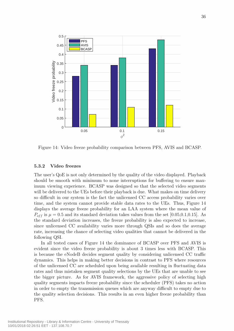
The user’s QoE is not only determined by the quality of the video displayed. Playbackshould be smooth with minimum to none interruptions for buffering to ensure max-imum viewing experience. BCASP was designed so that the selected video segmentswill be delivered to the UEs before their playback is due. What makes on time deliveryso difficult in our system is the fact the unlicensed CC access probability varies overtime, and the system cannot provide stable data rates to the UEs. Thus, Figure 14displays the average freeze probability for an LAA system where the mean value ofPoff is µ = 0.5 and its standard deviation takes values from the set [0.05,0.1,0.15]. Asthe standard deviation increases, the freeze probability is also expected to increase,since unlicensed CC availability varies more through QSIs and so does the averagerate, increasing the chance of selecting video qualities that cannot be delivered in thefollowing QSI.

In all tested cases of Figure 14 the dominance of BCASP over PFS and AVIS isevident since the video freeze probability is about 3 times less with BCASP. Thisis because the eNodeB decides segment quality by considering unlicensed CC trafficdynamics. This helps in making better decisions in contrast to PFS where resourcesof the unlicensed CC are scheduled upon being available resulting in fluctuating datarates and thus mistaken segment quality selections by the UEs that are unable to seethe bigger picture. As for AVIS framework, the aggressive policy of selecting highquality segments impacts freeze probability since the scheduler (PFS) takes no actionin order to empty the transmission queues which are anyway difficult to empty due tothe quality selection decisions. This results in an even higher freeze probability thanPFS.

Institutional Repository - Library & Information Centre - University of Thessaly10/01/2018 02:26:51 EET - 137.108.70.7

37

φ2

0.05 0.1 0.15

Vid

eo fr

eeze

dur

atio

n (s

)

0

0.2

0.4

0.6

0.8

1

1.2

1.4

1.6PFSAVISBCASP

Figure 15: Video freeze duration comparison between PFS, AVIS and BCASP.

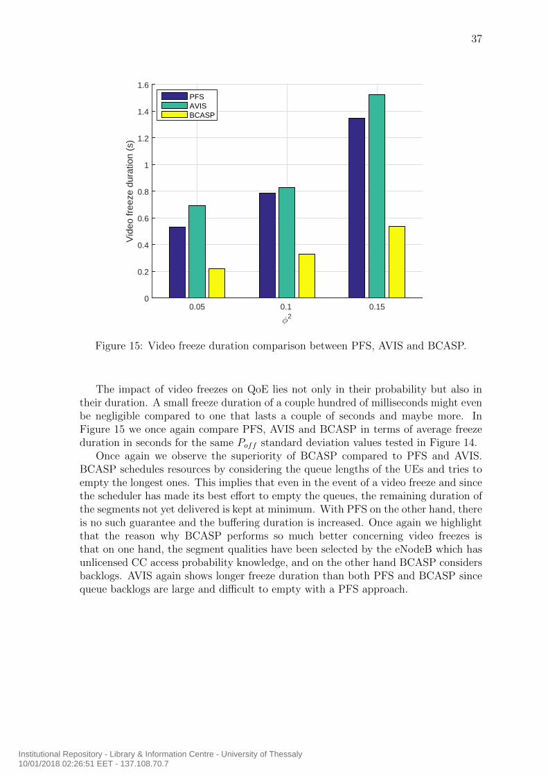
The impact of video freezes on QoE lies not only in their probability but also intheir duration. A small freeze duration of a couple hundred of milliseconds might evenbe negligible compared to one that lasts a couple of seconds and maybe more. InFigure 15 we once again compare PFS, AVIS and BCASP in terms of average freezeduration in seconds for the same Poff standard deviation values tested in Figure 14.

Once again we observe the superiority of BCASP compared to PFS and AVIS.BCASP schedules resources by considering the queue lengths of the UEs and tries toempty the longest ones. This implies that even in the event of a video freeze and sincethe scheduler has made its best effort to empty the queues, the remaining duration ofthe segments not yet delivered is kept at minimum. With PFS on the other hand, thereis no such guarantee and the buffering duration is increased. Once again we highlightthat the reason why BCASP performs so much better concerning video freezes isthat on one hand, the segment qualities have been selected by the eNodeB which hasunlicensed CC access probability knowledge, and on the other hand BCASP considersbacklogs. AVIS again shows longer freeze duration than both PFS and BCASP sincequeue backlogs are large and difficult to empty with a PFS approach.

Institutional Repository - Library & Information Centre - University of Thessaly10/01/2018 02:26:51 EET - 137.108.70.7

38

6 Conclusion

This work provides a framework for the application of adaptive video streaming overa LAA system. LAA is a key enabler for 5G radio communications towards increas-ing subscribers’ data rates and satisfying data rate demanding applications such asadaptive video streaming. To this end, the presented analysis exploits the extra un-licensed spectrum by placing segment quality decisions to the eNodeB, which hasunlicensed band activity knowledge. Quality selection is accomplished by employinga utility maximization problem at the eNodeB under resource allocation constraints.The problem is solved using the ADMM in linear to the number of users complex-ity and its solution determines the segment qualities to be delivered to the users forthe next interval. Furthermore, a scheduling policy that is ideal for delivering thepredetermined amount of payload under specific time constraints is employed. Thepolicy is based on Lyapunov optimization and its advantage is that it tries to scheduleresources to the users that not only experience high instant data rate, but also haveincreased queue backlogs, meaning that there are a lot of bits to be transmitted yet,for the segment download completion. This method is found to optimize performancecompared to a standard PFS approach as in two ways. Firstly, the users experiencehigher quality video with respect to the selected segment encoding rates and secondlythe amount and duration of video freezes, due to buffer under-run events that greatlyaffect viewing experience, is minimized. An existing adaptive video streaming frame-work that shares many similarities with the one proposed in this work is also employedfor comparison. The results indicate that although it generally provides higher seg-ment quality to the users, it is too aggressive resulting in increased buffer under-runprobability that causes disturbing and longer video freezes.

Institutional Repository - Library & Information Centre - University of Thessaly10/01/2018 02:26:51 EET - 137.108.70.7

39

References

[1] Qualcomm, “LTE Advanced-evolving and expanding in to new frontiers,” tech.rep., August, 2014.

[2] S. Han, Y.-C. Liang, and B.-H. Soong, “Spectrum refarming: A new paradigm ofspectrum sharing for cellular networks,” in Global Communications Conference(GLOBECOM), 2014 IEEE, pp. 893–898, Dec 2014.

[3] 3GPP, TR 36.889 TSG RAN, “Study on Licensed-Assisted Access to unlicensedspectrum,” Rel.13 v13.0.0, June 2015.

[4] T. Stockhammer, “Dynamic adaptive streaming over HTTP –: Standards anddesign principles,” in Proceedings of the Second Annual ACM Conference on Mul-timedia Systems, MMSys ’11, (New York, NY, USA), pp. 133–144, ACM, 2011.

[5] J. Zyren, “Overview of the 3GPP Long Term Evolution physical layer,” Tech.Rep. 3GPPEVOLUTIONWP, Freescale Semiconductor, Inc, July 2007.

[6] 3GPP, TS 36.106, “FDD repeater radio transmission and reception,” Release 8v8.3.0, 2009-2010.

[7] A. Galanopoulos, T. Tsiftsis, and F. Foukalas, “Licensed Assisted Access: Keyenabling functionalities and initial results,” in 2015 International Symposium onWireless Communication Systems (ISWCS), pp. 171–175, Aug 2015.

[8] A. Galanopoulos, G. Iosifidis, A. Argyriou, and L. Tassiulas, “Green video deliveryin LTE-based heterogeneous cellular networks,” in World of Wireless, Mobile andMultimedia Networks (WoWMoM), 2015 IEEE 16th International Symposium ona, pp. 1–9, June 2015.

[9] X. Wang, J. Chen, A. Dutta, and M. Chiang, “Adaptive video streaming overwhitespace: SVC for 3-tiered spectrum sharing,” in Computer Communications(INFOCOM), 2015 IEEE Conference on, pp. 28–36, April 2015.

[10] A. Abdel-Hadi and T. C. Clancy, “An optimal resource allocation with jointcarrier aggregation in 4G-LTE,” CoRR, vol. abs/1405.6448, 2014.

[11] T. Erpek, A. Abdel-Hadi, and T. C. Clancy, “An optimal application-aware re-source block scheduling in LTE,” CoRR, vol. abs/1405.7446, 2014.

[12] J. Chen, R. Mahindra, M. A. Khojastepour, S. Rangarajan, and M. Chiang,“A scheduling framework for adaptive video delivery over cellular networks,” inProceedings of the 19th Annual International Conference on Mobile Computing&#38; Networking, MobiCom ’13, (New York, NY, USA), pp. 389–400, ACM,2013.

[13] S. Wang, Q. Yang, W. Shi, and C. Wang, “Interference mitigation and resourceallocation in cognitive radio-enabled heterogeneous networks,” in Global Commu-nications Conference (GLOBECOM), 2013 IEEE, pp. 4560–4565, Dec 2013.

Institutional Repository - Library & Information Centre - University of Thessaly10/01/2018 02:26:51 EET - 137.108.70.7

40

[14] D. Bethanabhotla, G. Caire, and M. J. Neely, “Utility optimal scheduling andadmission control for adaptive video streaming in small cell networks,” CoRR,vol. abs/1305.3586, 2013.

[15] D. Bethanabhotla, G. Caire, and M. J. Neely, “Joint transmission scheduling andcongestion control for adaptive video streaming in small-cell networks,” CoRR,vol. abs/1304.8083, 2013.

[16] D. Bethanabhotla, G. Caire, and M. J. Neely, “Adaptive video streaming forwireless networks with multiple users and helpers,” IEEE Transactions on Com-munications, vol. 63, pp. 268–285, Jan 2015.

[17] Y. Li, F. Baccelli, J. G. Andrews, T. D. Novlan, and J. C. Zhang, “Modelingand analyzing the coexistence of Wi-Fi and LTE in unlicensed spectrum,” CoRR,vol. abs/1510.01392, 2015.

[18] G. Bianchi, “Performance analysis of the IEEE 802.11 distributed coordinationfunction,” IEEE Journal on Selected Areas in Communications, vol. 18, pp. 535–547, March 2000.

[19] G. Bianchi, “IEEE 802.11-saturation throughput analysis,” IEEE Communica-tions Letters, vol. 2, pp. 318–320, Dec 1998.

[20] X. Yin, A. Jindal, V. Sekar, and B. Sinopoli, “A control-theoretic approach fordynamic adaptive video streaming over HTTP,” SIGCOMM Comput. Commun.Rev., vol. 45, pp. 325–338, Aug. 2015.

[21] S. Boyd, N. Parikh, E. Chu, B. Peleato, and J. Eckstein, “Distributed optimiza-tion and statistical learning via the alternating direction method of multipliers,”Found. Trends Mach. Learn., vol. 3, pp. 1–122, Jan. 2011.

[22] R. Nishihara, L. Lessard, B. Recht, A. Packard, and M. I. Jordan, “A generalanalysis of the convergence of ADMM,” International Conference on MachineLearning, 2015.

[23] M. Carpin, A. Zanella, J. Rasool, K. Mahmood, O. Grøndalen, and O. N. Østerbø,“Scheduling policies for the LTE downlink channel: A performance comparison,”CoRR, vol. abs/1409.8633, 2014.

[24] M. J. Neely, Stochastic Network Optimization with Application to Communicationand Queueing Systems. Morgan & Claypool, 2010.

[25] M. T. Kawser, N. I. B. Hamid, M. N. Hasan, M. S. Alam, and M. M. Rahman,“Downlink SNR to CQI mapping for different multiple antenna techniques inLTE,” International Journal of Information and Electronics Engineering, vol. 2,no. 5, 2012.

Institutional Repository - Library & Information Centre - University of Thessaly10/01/2018 02:26:51 EET - 137.108.70.7