Measure Theory and Probability Theory

Stéphane Dupraz

In this chapter, we aim at building a theory of probabilities that extends to any set the theory of probability

we have for finite sets (with which you are assumed to be familiar). For a finite set with N elements Ω =

ω1, ..., ωN, a probability P takes any n positive numbers p1, ..., pN that sum to one, and attributes to any

subset S of Ω the number P(S) =∑i/ωi∈S pi. Extending this definition to infinitely countable sets such as N

poses no difficulty: we can in the same way assign a positive number to each integer n ∈ N and require that∑∞n=1 pn = 1.1 We can then define the probability of a subset S ⊆ N as P(S) =

∑n∈S pn.

Things get more complicated when we move to uncountable sets such as the real line R. To be sure, it is

possible to assign a positive number to each real number. But how to get from these positive numbers to the

probability of any subset of R?2 To get a definition of a probability that applies without a hitch to uncountable

sets, we give in the strategy we used for finite and countable sets and start from scratch.

The definition of a probability we are going to use was borrowed from measure theory by Kolmogorov in 1933,

which explains the title of this chapter. What do probabilities have to do with measurement? Simple: assigning

a probability to an event is measuring the likeliness of this event. What we mean by likeliness actually does

not matter much for the mathematics of probabilities, and various interpretations can be used: the objective

fraction of times an event occurs if we repeat some experiment an infinity of times, my subjective belief about

the outcome of the experiment, etc. From a mathematical perspective, what matters is that a probability is

just a particular case of a measure, and the mathematical theory of probabilities will at first be quite indifferent

to our craving to apply it to the measurement of hazard.

Although our main interest in measure theory is its application to probability theory, we will also be con-

cerned with one other application: the definition of the Lebesgue measure on R (and Rn), meant to correspond

for an interval [a, b] to its length b− a.

1The infinite sum is to be understood as the limit of the sequence∑N

n=1 pn. There is a subtlety because is not obvious thatthe limit is the same regardless of the ordering of the sequence, but it turns out that the invariance is guaranteed because the pn

are positive.2You may be thinking of using an integral, but we have not defined integrals in the class yet—we will do so in this very chapter

after defining probabilities on R. There is more to this than my poor organization of chapters: the integral that we could havebuilt before starting this chapter is the Riemann integral. But the Riemann integral is only defined on intervals of R, so that itcould only have helped us defining the probability of intervals. The integral we will build in this chapter from the definition of ameasure is the Lebesgue integral, a considerable extension of the Riemann integral.

1

1 Measures, probabilities, and sigma-algebras

We are looking for a notion to tell how big a set is, and whether it is bigger than another set. Note that we

already have one such notion: cardinalities. Indeed, for finite sets, we can compare the size of sets through

the number of elements they contain, and the notion of countability and uncountability extends the notion to

comparing the “size of infinite sets”.

Cardinalities have two limitations however. First, it restricts to a specific way of measuring the size of a

subset. Instead, maybe we want to put different weights on different elements, for instance in the context of

probabilities because some outcomes are deemed more likely than others. We are aiming at a more general

notion. Second, even restricting to some “uniform” measure, as soon as we reach the uncountable infinity,

cardinality makes very coarse distinctions between sizes: for instance R and [0, 1] have the same “size” according

to cardinality since they are in bijection. We would like to be able to say that R is bigger than [0, 1].

So let us build a new notion, that of a measure. In essence, what we want a measure on a set Ω to do is to

assign a positive number (or infinity) to subsets of Ω. Really, there is only one property that we wish to impose:

that the union of two disjoint subsets be the sum of the measures of the two subsets—additivity. By induction,

additivity for 2 disjoint subsets is equivalent to additivity for a finite number of pairwise disjoint subsets. What

about infinite unions? Well, why not, but note that we have no clue what the sum of an uncountable infinity

of positive numbers is—we have never defined such a notion. So we require additivity for pairwise disjoint

countable collection of subsets—sigma-additivity.

Definition (provisory). Let Ω be a set. A measure µ on Ω is a function defined on P(Ω) which:

1. Takes values in R+ ∪ +∞, and such that µ(∅) = 0.

2. Is sigma-additive (countably-additive): for any countable collection of subsets (An)n∈N of Ω that

are pairwise disjoint (Ai ∩Aj = ∅ for all i 6= j),

µ

( ∞⋃n=1

An

)=∞∑n=1

µ(An).

Now there is a reservation, which is why the definition has been labeled “provisory”. For some sets, such

as finite and countable sets, this definition would be quite good. But as it is, it would quickly put us in

trouble when dealing with uncountable sets such as the real line R. To understand why, and to understand

the little detour that we are going to make before giving the proper definition of a measure—the definition

of sigma-algebras—it is useful to consider the problem Lebesgue was trying to solve in 1902. Lebesgue was

trying to extend the notion of the length of an interval to all subsets of R. To this end, he asked whether there

2

exists a positive function µ on the power set of R that is sigma-additive—a measure according to our provisory

definition, invariant by translation (meaning µ(S + x) = µ(S) for all subset S ⊂ R and vector x ∈ R), and

normalized by µ([0, 1]) = 1. This does not sound like asking for much, but unfortunately, in 1905, Vitali showed

that there is no such function.

The way mathematicians reacted to this drawback has been to allow for a measure to be defined on only a

collection of subsets smaller than the entire power set, restricting the subsets that can be measured. But not

on any collection of subsets of Ω; only on collections that satisfy a few properties: sigma-algebras.

1.1 Sigma-algebras

We are willing to restrict the collection of measurable sets, but there are things on which we are not ready

to negotiate. First, if a set is measurable, we want its complement to be measurable too. (In the case of a

probability, if we give a probability to an event happening, we want to be able to give a probability to the event

not happening). Second, since we want our measures to be sigma-additive, we want the countable union of

measurable sets to be measurable. These requirements define a sigma-algebra.

Definition 1.1. Let Ω be a non-empty set. A collection A of subset of Ω is a sigma-algebra if:

1. Ω ∈ A.

2. It is close under complementation: A ∈ A ⇒ Ac ∈ A.

3. It is close under countable union: (An)n∈N ∈ A ⇒⋃n∈NAn ∈ A.

Elements of a sigma-algebra A are called measurable sets.

The couple (Ω,A) is called a measurable space.

Note that a sigma-algebra also necessarily:

• Contains the empty-set (since ∅ = Ωc).

• Is close under countable intersection (using Morgan’s law and closeness under countable union and com-

plementation).

It is easy to build sigma-algebras. For instance, in the set Ω = 1, 2, 3, ∅,Ω is a sigma-algebra, as

are ∅, 1, 2, 3,Ω and P(Ω). More generally, on any set Ω, the collection Ω, ∅ is a sigma-algebra—it

is the coarsest sigma-algebra since it is the one that allows to measure the fewer subsets. Also, P(Ω) is a

sigma-algebra—it is the finest sigma-algebra since it allows to measure all subsets. The whole point of defining

3

sigma-algebras however is to end up with a collection of sets that is smaller than P(Ω). On this account, be

careful that only countable unions (intersections) of measurable sets are required to be measurable: asking for

sigma-algebra to be close under any union would considerably restrict the number of sigma-algebras we can

define on a set. For instance, were we to require all singletons of a set Ω to me measurable, we would fall back

on P(Ω).

How to generate sigma-algebras? Let us import a trick we used in linear algebra to create vector subspaces.

There, we saw that given any subset S of a vector space, we can always define the vector subspace generated

by S as the smallest vector subspace containing S—the intersection of all vector subspaces containing S. What

allowed us to do this was that any (possibly infinite) intersection of vector subspaces is a vector subspace. It is

easy to check that similarly, any (possibly infinite—possibly uncountably infinite for that matter) intersection

of sigma-algebras is a sigma-algebra. So that we can define the sigma-algebra generated by any subset S of

P(Ω).

Definition 1.2. Let S be a collection of subset of the set Ω.

The sigma-algebra generated by S, noted σ(S), is the smallest sigma-algebra that contains S, or:

σ(S) =⋂A,A is a sigma-algebra and S ⊆ A

We are now ready to define the sigma-algebra that we will use in practice to define all our measures on

R: the Borel sigma-algebra. The logic behind the definition is simple: we want our measures to be able to

measure the open intervals (a, b) of R. However, this is not a sigma-algebra—just consider the union of two

disjoint open intervals—so we take the sigma-algebra generated by the open intervals of R. It is easy to check

that the sigma-algebra generated by the open intervals of R is equivalently the sigma-algebra generated by the

open set of R (you are asked to check it in the problem-set), so that the definition of the Borel sigma-algebra

is frequently phrased as the sigma-algebra generated by the open sets of R.

Definition 1.3.

The Borel sigma-algebra on R, noted B(R), is the sigma-algebra generated by the open sets of R.

Equivalently, it is the sigma-algebra generated by the open intervals (a, b) of R.

The Borel sigma-algebra on Rn, noted B(Rn), is the sigma-algebra generated by the open sets of Rn.

Equivalently, it is the sigma-algebra generated by the setsn∏i=1

(ai, bi) of Rn.

A measurable set of the Borel sigma-algebra is called a Borel set.

(To be clear: we are referring to the open sets for the Euclidian distance in Rn—the absolute value in R). The

open sets of R do not form more of a sigma-algebra than the set of finite open intervals of R—if so, it would

4

need to include all closed sets, and it does not—so the Borel set is a bigger collection of sets than the collection

of open sets of R. Actually, finding a non-measurable set according to the Borel sigma-algebra is rather hard,

but Vitali showed such sets exist (the counterexamples he used are now called Vitali sets). Simply put, the

Borel sigma-algebra is quite huge but is not the whole power set of R, so that it makes it a perfect candidate

to define measures on. From now on, anytime we talk of R and Rn, it is to be understood as the measurable

space (R,B(R)) and (Rn,B(Rn)).

1.2 Measures

We are now ready to give the proper definition of a measure: it only generalizes the provisory definition given

above to allow probabilities to be defined on a sigma-algebra of Ω that is not necessary the power set of Ω.

Definition 1.4. Let (Ω,A) be a measurable set. A measure µ on (Ω,A) is a function defined on A which:

1. Takes values in R+ ∪ +∞, and such that µ(∅) = 0.

2. Is sigma-additive: for any countable collection (An)n∈N of A that are pairwise disjoint:

µ

( ∞⋃n=1

An

)=∞∑n=1

µ(An).

The triple (Ω,A, µ) is called a measure space.

It is easy to check that on any finite set Ω, the number of elements in a subset is a measure on (Ω,P(Ω)). It

can be generalized to countably infinite sets: on N, the measure that associates the number of elements in a

subset, or ∞ if the set is infinite, is a measure on (N,P(N)). It is called the counting measure.

Below are three essential properties of a measure.

Proposition 1.1. A measure µ on (Ω,A) satisfies the following properties:

1. Monotonicity: Let A,B ∈ A. A ⊆ B ⇒ µ(A) ≤ µ(B).

2. Sigma-sub-additivity: for any countable collection (An)n∈N ∈ A, µ( ∞⋃n=1

An

)≤∞∑n=1

µ(An).

3. “Continuity property”: If An is an increasing sequence for ⊆ (meaning An ⊆ An+1 for all n),

then µ( ∞⋃n=1

An

)= limn→∞ µ(An).

Proof. All three proofs consist in re-partitioning the sets so as to end up with disjoint sets, and use sigma-

additivity.

5

• Monotonicity: write B = A∪ (B−A). Since A and B −A are disjoint, µ(B) = µ(A) + µ(B−A) ≥ µ(A).

• Sigma-sub-additivity: define the disjoint sequence of sets (Bn)n as Bn = An −⋃n−1k=1 Ak. We have that

∞⋃n=1

An =∞⋃n=1

Bn and µ(Bn) ≤ µ(An) for all n, so µ( ∞⋃n=1

An

)= µ

( ∞⋃n=1

Bn

)=∞∑n=1

µ(Bn) ≤∞∑n=1

µ(An).

• Define the pairwise disjoint collection of sets Bn = An − An−1 (and B1 = A1), so that An =n⋃i=1

Bi and

∞⋃i=1

Ai =∞⋃i=1

Bi. Then using sigma-additivity twice:

µ(An) = µ

(n⋃i=1

Bi

)=

n∑i=1

µ(Bi)→∞∑i=1

µ(Bi) = µ

( ∞⋃i=1

Bi

)= µ

( ∞⋃i=1

Ai

).

The continuity property is really a particular application of sigma-additivity, but a very useful one to find the

measure of a set. To find the measure of a set A, if we can write A as the limit of an increasing sequence of sets

An the measure of which we know, then we can find µ(A) as the limit of the real-valued sequence (µ(An))n.

Finally, just a piece of vocabulary. We think of sets of measure zero as negligible. So if a property is true

everywhere except on a set of measure zero, we want to say that it is “almost true”. To make such statements

rigorous, we define the notion of true almost everywhere.

Definition 1.5. A property is true almost everywhere, abbreviated a.e., if the set on which it is false

has measure zero.

1.3 Probabilities

Let us come back to our main interest: probabilities. From a mathematical perspective, a probability is just a

particular case of a measure on a set: one such that the whole set has size one. There is nothing in the definition

of a probability that stresses that we will apply such measures to measuring the likeliness of events.

Definition 1.6.

• A measure such that µ(Ω) is finite is called a finite measure.

(If so, using monotonicity, any measurable subset has finite measure).

• A (finite) measure such that µ(Ω) = 1 is called a probability.

6

When dealing with a probability:

• we call events the measurable sets of the associated sigma-algebra.

• we call the measure space a probability space.

• we say that a property is true almost surely (a.s.) if it is true on a set of probability 1.

The only difference between a finite measure and a probability is the cosmetic additional requirement of the

normalization of µ(Ω) to 1. There is nothing more complicated, but also nothing to gain, in studying finite

measures that are not normalized to one, and so we restrict to probabilities only. Let us just add one definition,

which is not nearly as important as finite measure, but will show up as a technical requirement in theorems

below.

Definition 1.7. Let µ be a measure on a measurable set (X,A).

µ is sigma-finite if there exists a countable family of subsets (Ak)k ∈ A of finite measure µ(Ak) <∞

for all k, such that X ⊆∞⋃k=1

Ak.

A probability—a finite measure—is necessarily sigma-finite.

7

2 Defining measures by extension on Rn

To define probabilities on a countable set, we usually take the sigma-algebra on Ω to be the entire power set

P(Ω). On such a measurable space, a probability P is entirely characterized by the probabilities pω = P(ω)

that it assigns to each singleton ω—equivalently to each element ω. Indeed, given positive numbers (pω)

for all singletons, sigma-additivity allows to recover the probability of all subsets of Ω, since any subset is the

countable union of its elements. The only requirement is that P(Ω) = 1: that the pω’s sum to one. Thus, our

definition of a probability chimes with the one we gave in the introduction for finite and countably infinite sets.

The benefit of our new definition is that it also applies to uncountable sets such as the real line R, where we

would have no way to extend a probability from singletons to Borel sets.

But our general definition of a probability—and more generally of a measure—is not constructive: in practice,

how to define a measure on R and Rn? The strategy we are going to adopt is not so different from the one we

used for countable sets: we are going to define our measures on a simple collection of subsets of R or Rn, and

then extend it to the whole Borel sigma-algebra.

2.1 Carathéodory’s extension theorem

Two questions then. First, what simple collection of sets? Simple: remember that we defined the Borel sigma-

algebra as the one generated by open intervals (a, b) of R. So we are going to pick intervals as our simple

collection of sets. There is one technical subtlety however. For technical reasons, it is more practical to use

right-semiclosed intervals (a, b]. As is easily checked, they too generate the Borel sigma-algebra. In this course—

the notation is not universal—we will note I the set of all right-semiclosed intervals (a, b], and more generally

In for the corresponding set on Rn.

I = (a, b], a, b ∈ R ∪ ±∞, a < b ∪ ∅

In =

n∏i=1

(ai, bi], ai, bi ∈ R ∪ ±∞, ai < bi for all i∪ ∅

Note that we impose a < b since (a, a] would not make sense, and that we allow a and b to be ±∞; in particular

Rn belong to In. Also, note that we add the empty set to In.

Second, how to extend our measure? We will not dig too much into the details here, and instead admit the

following theorem, that gives the existence and uniqueness of an extension of a measure from I to B(R).

8

Theorem 2.1. (Carathéodory’s extension theorem on Rn). Let µ be a function from In to R. If:

1. µ is a “measure” on In (“measure” is a bit abusive since In is not a sigma-algebra), that is:

(a) µ takes values in R+ ∪ +∞, and µ(∅) = 0.

(b) µ is sigma-additive on In: for all (Ak)k∈N ∈ In pairwise disjoint, if⋃k∈NAk ∈ In,

µ

( ∞⋃k=1

Ak

)=∞∑k=1

µ(Ak).

2. µ is sigma-finite.

Then there exists a unique measure µ∗ on (Rn,B(Rn)) such that µ(A) = µ∗(A) on all A ∈ In.

Proof. Admitted.

The uniqueness part of the Carathéodory theorem tells us that a measure is characterized by its values on In:

if two measures coincide on In, then they are equal on the whole Borel set B(Rn). The existence part of the

Carathéodory theorem tells us that it is possible to extend a measure from In to Rn. Thus, when defining a

measure, it is enough to define the values the measure takes on In. We turn to two applications of this: defining

probabilities on R, and defining the Lebesgue measure on Rn.

2.2 Application 1: defining probabilities on R through their CDF

Let us consider the case of probabilities on R. Because a probability is a finite measure, we can simplify the

problem further: it is enough to define a probability P on the set J ⊆ I of intervals of the form (−∞, x], x ∈ R.

Indeed, for a < b, (−∞, b] = (−∞, a]∪ (a, b], so P((a, b]) = P((−∞, b])−P((−∞, a]). Thus, from the knowledge

of P on J , we can back out the values of P on I.3 Why is J an improvement with respect to I? Because,

since the intervals (−∞, x] are indexed by a single number x, we can sum up all the information that we need

to define P through a single-variable function. (For x = ±∞, we always have P((−∞,−∞)) = P(∅) = 0 and

P((−∞,+∞)) = P(R) = 1). Given a probability P defined on B(R), we call this function the cumulative

distribution function of P.

Definition 2.1. The cumulative distribution function (CDF) F of a probability P is the function

3The fact that P is finite intervenes in excluding the possibility of an indeterminate form P((a, b]) =∞−∞.

9

from R to [0, 1] defined as:

∀x ∈ R, F (x) = P((−∞, x])

As an immediate corollary of the uniqueness part of the Carathéodory theorem, we know that the CDF of a

probability P characterizes P: two probabilities that have the same CDF define the same function on J , hence

on I, hence on B(R), thus are equal. The existence part of the theorem can help us to characterize the functions

F that correspond to a probability.

Proposition 2.1. A function F from R to [0, 1] is a CDF of a probability P on R if and only if it is:

1. Increasing.

2. Right-continuous (everywhere): ∀x0,∀ε > 0,∃δ > 0/0 ≤ x− x0 < δ ⇒ |f(x)− f(x0)| < ε.

3. With limit 0 in −∞ and limit 1 in +∞.

Proof. We are going to skip to proof, but roughly: F increasing parallels the monotonicity of P, F right-

continuous parallels the continuity property of P, and the limits in ±∞ parallel the measure of the empty set

and the whole real line.

Be careful that a CDF does not need to be left-continuous (hence continuous). For instance if we flit a coin and

gain one dollar with probability 1/2, and lose one dollar with probability 1/2, that associated CDF on R will

be discontinuous at 0 and 1, jumping from 0 to 1/2, and from 1/2 to 1.

2.3 Application 2: the Lebesgue measure on Rn

We now turn to the only infinite measure—meaning that it assigns an infinite measure to some sets—that we

will be concerned with in this chapter: the Lebesgue measure. The Lebesgue measure is meant to capture the

“natural” measure on the real line R. What we mean by natural is that it corresponds for an interval (a, b] to its

length b−a (and if the interval is unbounded—a = −∞ or b = +∞—the measure is infinite). It is easy to check

that this measure defined on I is sigma-additive on I and sigma-finite (R =⋃n∈Z(n, n+ 1]), so Carathéodory

theorem tells us that it extends uniquely to a measure defined on B(R).

Definition 2.2.

10

The Lebesgue measure λ on R is the unique extension to B(R) of the function defined on I as:

λ((a, b]) = b− a (and +∞ if a = −∞ or b = +∞).

The Lebesgue measure λ on Rn is the unique extension to B(Rn) of the function defined on In as:

λ

(n∏i=1

(ai, bi])

=n∏i=1

(bi − ai) (and +∞ if ai = −∞ or bi = +∞ for some i).

The notation λ for the Lebesque measure is standard, although be careful that λ if sometimes used to designate

other measures as well.

One remark: the Lebesgue measure is actually slightly extended in the following way. Define N as the

collection of all subsets of R (not necessarily Borel-measurable) that are included in a Borel set of Lebesgue

measure zero: A ⊆ B, λ(B) = 0. It is possible to show that B(R) ∪ N is a sigma-algebra. We add N to the

collection of sets on which we define the Lebesgue measure, and define the measure of the subsets in N to be

zero.

Another remark, as names may be intriguing you: does the Lebesgue measure on R solve the Lebesgue

problem? Yes: it is sigma-additive and normalized to 1, and can be shown to be invariant by translation (that

it is invariant by translation on I is straightforward). It can also be shown to be the only measure that satisfy

these three properties.

Here are some results that are useful to get a better sense of the Lebesgue measure.

Proposition 2.2.

• Any singleton of R has Lebesgue-measure zero.

• Any countable set of R—in particular N and Q—has Lebesgue-measure zero.

• There are also uncountable sets of R that have a zero Lebesgue-measure.

Proof.

• Let a be a singleton. Since (a − 1, a] = (a − 1, a) ∪ a, which are disjoint sets, if we show that

λ((a − 1, a)) = 1 we are done since then λ(a) = λ((a − 1, a]) − λ((a − 1, a)) = 1 − 1 = 0. Write

(a − 1, a) =⋃∞n=1(a − 1, a − 1

n ]. The sets (a − 1, a − 1n ] are increasing so by the continuity property,

λ((a− 1, a)) = limn→∞ λ((a− 1, a− 1n )] = limn→∞ 1− 1

n = 1. QED.

• It is then a direct consequence of sigma-additivity that countable sets have measure zero.

11

• You will see an example in the problem-set.

Note that the fact that countable sets have zero Lebesgue measure seems reminiscent of the insight from

cardinality theory that countable infinity is “negligible” in front of uncountable infinity. But the last item in

the proposition warns us against the perils of the analogy between cardinality and the Lebesgue measure: the

Lebesgue measure also sees as “negligible”—meaning of measure zero—some uncountable sets.

12

3 Defining measures by image

An alternative way to define a measure on a measurable space (Y,B) is by importing a measure µ from another

measurable space (X,A) where µ is defined. Consider the example of playing (European) roulette. We can

model it through a sample space Ω consisting of the 37 outcomes:

Ω = the ball falls into 0, the ball falls into 1, ..., the balls falls into 36

We can turn Ω into a measurable space by coupling it with the sigma-algebra P(Ω), and into a measured space

by adding for instance the uniform probability P that assigns 1/37 to each outcome. Now Roulette is only fun

if there is something at stake, so let us assume we bet $1 on number 25 so that we win $35 if the ball falls into

25, and lose $1 if it falls into anything else. It is natural to define the payoff function f from Ω to R:

f : Ω→ R

the ball falls into 25 7→ 35

any other outcome 7→ −1

You may have already calculated that our probability of getting $35 is 1/37, and our probability of getting -$1

is 36/37. But do note how we come up with these numbers. To come up with 1/37, we sum up the probabilities

of all the outcomes that lead to a payoff of 35—there is only one. To come up with 36/37, we sum up the

probabilities of all the outcomes that lead to a payoff of -$1. We could also calculate the probability of getting

any other real number x as a payoff: there is no outcome that leads to such payoff, so the probability would be

P(∅) = 0. We could also get the probability of getting less than $50 dollar, or of any event—any measurable

subset S of R. In all cases, the logic would be to sum the probabilities of all the outcomes of Ω such that the

payoff is in S. In other words, we define a probability Q on the real line as the probability of its inverse image.

∀B ∈ B(R),Q(B) = P(f−1(B))

This way of defining a measure is very general: given any two measurable sets (X,A) and (Y,B), we can define

a new measure on (Y,B) from a measure µ on (X,A) as long as we have a function f such that the inverse

image of any measurable set of Y is a measurable set of X. This leads us to define measurable functions.

3.1 Measurable functions

13

Definition 3.1. Let (X,A) and (Y,B) be two measurable spaces, and f : X → Y a function.

f is a measurable function if the inverse images by f of a measurable set of Y is a measurable set of X:

∀B ∈ B, f−1(B) ∈ A

Note that the definition of a measurable function makes no reference to the existence of a measure on either

set.

3.2 Image measure

So now, here is our general result:

Proposition 3.1.

Let (X,A, µ) be a measure space, (Y,B) be a measurable space, and f : X → Y a measurable function.

The function µf on (Y,B) defined by:

µf (B) = µ(f−1(B)) for all B ∈ B

is a measure on (Y,B), called image measure of µ under f .

Proof. The function µf is positive and µf (∅)=µ(f−1(∅)) = µ(∅) = 0. As for sigma-additivity, let (Bn) be a

countable family of pairwise disjoint measurable sets:

µf

( ∞⋃n=1

Bn

)= µ

(f−1

( ∞⋃n=1

Bn

))= µ

( ∞⋃n=1

f−1(Bn))

=∞∑n=1

µ(f−1(Bn)) =∞∑n=1

µf (Bn)).

3.3 Random variables

As always, probability theory is ashamed of just being a particular case of measure theory, and insists on having

its own vocabulary.

Definition 3.2. Let (Ω,A) and (Y,B) be two measurable spaces.

When the measures we deal with on (Ω,A) and (Y,B) are probabilities:

• We call a measurable function a random variable and usually note it X.

14

• When (Y,B) is (R,B(R)), we call X a real random variable.

• When (Y,B) is (Rn,B(Rn)), we call X a random vector.

• We call the image probability of a probability P on Ω under X the probability of the random

variable X, and note it PX .

Remember that a probability on R is characterized by its CDF. Noting FX the CDF of PX , we have:

∀x ∈ R, FX(x) = PX((−∞, x]) = P(X−1((−∞, x]) = P(ω ∈ Ω/X(ω) ∈ (−∞, x]) = P(ω ∈ Ω/X(ω) ≤ x)

FX(x) = P(X ≤ x)

So the vocabulary is different when we deal with probabilities. But also, the vocabulary is weird: the term

variable is not very descriptive of what it names—a function. And the practice of probability theory adds to

the confusion: theorems and exercises often start with “Let X be a random variable with CDF given by...”,

while remaining silent on what the domain Ω of the function X is, and not really using at any point that X is

a function.

Here is why we can do so: very often, we do not really care about the set Ω and the function X. They are

only instrumental objects in defining a probability on (Y,B). Once we have used them to define PX , we can just

as well toss them aside. Actually, we could as well start by defining a probability on (Y,B) directly through its

CDF, without any reference to a set Ω or a function X. For instance, in the roulette example above, we could

have started by directly defining the probability Q on the real line.

Why we do keep referring to our probability Q as the one associated to a function X defined of an implicit

set Ω is just because it is a convenient way of thinking about it in our application of probability theory to

hazard. We like to think of our probability Q on the real line as resulting—through a function—from some

source of randomness in some set Ω. What is Ω? The roulette, the world, the universe: it is not very clear—but

also it does not need to be very clear since only the image probability Q matters. And it is why we do not

bother stating what Ω is.

15

4 Lebesgue Integral and expectations

You have seen a theory of integration—the Riemann integral—defined for continuous functions on a segment

[a, b] of the real line. Measure theory allows to build a theory of integration—the Lebesgue integral—that fits

the Riemann integral when integrating a continuous function on a segment of the real line with respect to

the Lebesgue measure. But the Lebesgue integral is a considerable generalization: it is defined for (almost)

any measurable function from a measurable subset of a measure space to R, and can be defined for different

measures, not only the Lebesgue measure. (Don’t be confused by vocabulary: the Lebesgue integral does not

need to be taken with respect to the Lebesgue measure).

4.1 Sketch of the construction of the integral

We will note enter the details of the construction of the Lebesgue integral, but simply sketch the steps. Fist,

some definitions:

Definition 4.1. Let (X,A) be a measurable space.

• The indicator function of a measurable set A ∈ A, noted 1A is the real function defined on X as

1A(x) = 1 if x ∈ A and f(x) = 0 if x 6∈ A.

• A simple function is a finite linear combination of indicator functions of measurable sets:

f =n∑i=1

ai1Ai, ai ∈ R, Ai ∈ A,∀i = 1, ..., n.

Consider a measure space (X,A, µ). We will note the integral of a function f ,∫fdµ, or

∫f(x)dµ(x), which

makes explicit the dependence of the integral in the measure with respect to which the integral is taken. The

construction of the Lebesgue integral is in three steps.

1. Define the integral of a positive simple function f =n∑i=1

ai1Ai, ai ≥ 0 for all i, with respect to µ as:

∫fdµ =

n∑i=1

aiµ(Ai).

2. Extend the definition to positive measurable functions. To do so, we show that any positive measurable

function can be approximated as the (pointwise) limit of a (pointwise) increasing sequence (fn) of positive

simple functions. We show that the sequence (∫fndµ) converges in R ∪ +∞, and that the limit is

16

independent of the choice of the approximating sequence (fn). We define the integral of f as the common

limit. We say that f is integrable if its integral is finite:∫fdµ < +∞.

3. Extend the definition to (almost) all measurable function, not necessarily positive. To do so, we define

two measurable positive functions f+ and f− as: f+(x) = f(x) if f(x) ≥ 0 and f(x) = 0 otherwise;

f−(x) = −f(x) if f(x) ≤ 0 and f(x) = 0 otherwise. We can therefore decompose f = f+ − f−. When∫f+dµ <∞ or

∫f−dµ <∞, we define the integral of f as:

∫fdµ =

∫f+dµ−

∫f−dµ

(We cannot define the integral when both∫f+dµ =∞ and

∫f−dµ =∞). We say that f is integrable

if both f+ and f− are finite, or equivalently if |f | is integrable (∫|f |dµ <∞).

The Lebesgue integral generalizes the Riemann integral when the measure space is the real line endowed with the

Borel sigma-algebra and the Lebesgue measure. We therefore often note∫f(x)dx for the integral with respect

to the Lebesgue measure∫f(x)dλ(x). But the Lebesgue integral is not restricted to the Lebesgue measure,

not even the measurable space (R,B(R)). For instance, consider the measure space (N,P(N), µ), where µ is

the counting measure. Then any function from N to R—any real sequence—is measurable, and the Lebesgue

integral of an integrable sequence (xn) is∞∑n=1

xn. Some basic properties of the Lebesgue integral:

Proposition 4.1. Let (X,A, µ) be a measure space.

• The integral is linear: if f and g are integrable, and α, β ∈ R, then αf + βg is integrable and:

∫(αf + βg)dµ = α

∫fdµ+ β

∫gdµ.

• The integral is monotonic: for f and g integrable, if f ≤ g, then∫fdµ ≤

∫gdµ.

• If two integrable functions f and g are equal almost everywhere, then∫fdµ =

∫gdµ.

Proof. Admitted.

4.2 Monotone convergence theorem and Dominated convergence theorem

In this section, we gather results that allow to “permute the integral and the limit”, or “permute the integral

and differentiation”. Let us start with the limit. In parallel with the construction of the integral, there are two

17

results: one for positive measurable functions—the monotone convergence theorem—and one for any integrable

function—the dominated convergence theorem.

Theorem 4.1. Monotone Convergence Theorem

If (fn) is an increasing sequence of positive measurable functions that tends almost everywhere to f

(which may be defined as +∞ in some points), then f is measurable and limn→∞∫fndµ =

∫fdµ.

Proof. Admitted.

Theorem 4.2. Dominated Convergence Theorem

If (fn) is a sequence of measurable functions that tends almost everywhere to f , and there exists an

integrable function g such that |fn| ≤ g for all n, then f is integrable and limn→∞∫fndµ =

∫fdµ.

(Note that the fn are guaranteed to be integrable by the monotonicity of the integral).

Proof. Admitted.

Given that the derivative of a function from R to R is defined as a limit, it may not be too surprising that

we can deduce from the dominated convergence theorem a theorem that allows us to permute integration and

differentiation. To state it, consider the Borel sigma-algebra and the Lebesgue measure on the real line, and

consider a function f of two real variables: one with respect to which we integrate—t—and one with respect to

which we differentiate—x. When integrating over t, we obtain a function h(x) of the single variable x.

Proposition 4.2. Let f : R2 → R such that t 7→ f(t, x) is integrable for all x ∈ R.

Note h(x) =∫f(t, x)dt.

If x 7→ f(t, x) is differentiable for all t, and there exists an integrable function g such that | ∂∂xf(t, x)| ≤ g(t),

then h is differentiable and:

h′(x) = d

dx

∫f(t, x)dt =

∫f ′x(t, x)dt

Proof. Admitted.

4.3 Double integrals and Fubini theorem in R2

One way in which the Lebesgue integral is more general than the Riemann integral is that it painlessly defines

an integral on Rn, with respect to the Lebesgue measure of Rn. For instance in R2, we can consider a function

18

f(x1, x2) of two variables, and take its integral with respect to the Lebesgue measure of R2. Now, you might

also want to consider the real number obtained by first, for each value of x2, integrating f with respect to its

first variable x1 (with respect to the Lebesgue measure in R), and second integrating the resulting function of

x2 with respect to x2 (with respect to the Lebesgue measure in R). Or you might want to do the same thing

permuting the order of x1 and x2. Thus we can calculate three real numbers. Fubini’s theorem guarantees that

these three numbers are equal (if f is integrable). The result is twofold. First it gives us a way to calculate the

integral of a function of two variables in practice, integrating along each variable successively. Second, it allows

us to permute the order of integration when facing double integrals.

Theorem 4.3. (Fubini’s theorem) Let f : (R2,B(R2))→ (R,B(R)) be a measurable function.

If f is integrable (with respect to the Lebesgue measure in R2), then:

∫R2f(x1, x2)dλ(x1, x2) =

∫R

(∫Rf(x1, x2)dλ(x1)

)dλ(x2)

=∫R

(∫Rf(x1, x2)dλ(x2)

)dλ(x1).

(The theorem implicitly guarantees that the one-variable functions on the right-hand sides are integrable).

Proof. Admitted.

Fubini theorem is easily extended to integration in Rn, except that the notations get messier. In particular, we

can permute the order of integration in any way.

4.4 Integral wrt. an image measure

Consider the case of a measure ν on a measurable space (Y,B) defined as the image measure of a measure µ on

a measurable space (X,A) under the measurable function φ : X → Y . The integral with respect to ν can be

expressed as an integral with respect to µ.

Proposition 4.3. Let (X,A) and (Y,B) be two measurable spaces.

Let φ be a measurable function from X to Y , µ a measure on (X,A), ν the image measure of µ under φ.

Then for any integrable function f : Y → R,

∫Y

fdν =∫X

(f φ)dµ.

Proof. This is easy to check for indicator function:∫Y1Bdν = ν(B) = µ(φ−1(B) =

∫X1φ−1(B)dµ =

∫X

(1φ)dµ.

The proof—that we admit—then generalizes the result to any measurable function.

19

4.5 Expectations

Once again, probability theory has its own vocabulary: if (Ω,A,P) is a probability space, we call the integral

of a real random variable X from Ω to R the expectation of X, noted E(X).

Definition 4.2. Let (Ω,A,P) be a probability space, and X a real random variable from Ω to R. If X is

integrable, we call its integral the expectation of X, and note it E(X):

E(X) =∫

ΩX(ω)dP(ω)

Now remember that from the random variable X we can define the probability PX of X on R as the measure

image of P under X. Then, simply applying proposition 4.3 for f = Id, we get that:

E(X) =∫RxdPX(x)

It follows that the expectation of a random variable depends only on the probability PX . This is no surprise:

we have seen that once we have defined PX from P and X, we could just as well get rid of P, X and Ω. More

generally, for any function f : R→ R, f X is integrable wrt. P if and only if f is integrable wrt. PX , and:

E(f(X)) =∫

Ωf X(ω)dP(ω) =

∫Rf(x)dPX(x).

The expectation of f(X) when f is a power function plays an important role:

Definition 4.3. Provided they exist, we define for a real random variable X:

• The raw moment of order p: E(Xp).

• The central moment of order p: E((X − E(X))p).

We call the central moment of order 2 the variance: V (X) = E((X − E(X))2). Note the two following results

about the variance:

• V (X) = E(X2)− E(X)2.

(V (X) = E((X − E(X))2) = E(X2 − 2XE(X)− E(X)2) = E(X2)− 2E(X)2 − E(X)2 = E(X2)− E(X)2).

• V (X) = 0 if and only if X is almost surely constant.

(Admitted).

20

5 Densities

5.1 Defining measures trough densities

From any measure µ on a measurable set (X,A), we can define a new measure for any positive measurable

function f .

Definition 5.1. Let (X,A, µ) be a measure space. The function:

ν : A → R+ ∪ +∞

A 7→∫1Afdµ

is a measure on (X,A), called measure induced by the density f with respect to µ.

If∫fdµ = 1, f induces a probability; f is then also called a probability density function (PDF).

Proof. We admit that this defines a measure.

The integral of a function g with respect to ν can be expressed as an integral with respect to µ:

Proposition 5.1. Let ν be the measure induced by the density f wrt. µ.

For any measurable function g from (X,A) to (R,B(R)),

∫gdν =

∫g × fdµ.

Proof. Admitted.

For this reason, the density f is sometimes noted dνdµ .

5.2 The Radon-Nikodyn theorem

Given two measures µ and ν on (X,A), can we always find a measurable positive function f such that ν has

density f with respect to µ? The following reasoning shows that we cannot: if there exists a measurable set

A such that ν(A) > 0 but µ(A) = 0, then no f will do. Indeed, for all f ,∫1Afdµ = 0 6= ν(A). However,

the Radon-Nikodyn theorem guarantees that except for these measures ν that attribute measure zero to sets of

positive µ-measure, we can. Let us first give a name to the measures that will work.

21

Definition 5.2. Let (X,A, µ) be a measure space.

A second measure ν on (X,A) is absolutely continuous wrt. µ if:

∀A ∈ A, µ(A) = 0⇒ ν(A) = 0.

Theorem 5.1. (Radon-Nikodyn theorem)

Let (X,A) be a measurable space and µ and ν two measures on (X,A).

If µ and ν are both sigma-finite, and ν is absolutely continuous wrt. µ, then ν has a density wrt. µ.

The density is unique up to a µ-null set, i.e. any two densities are equal except on a set of measure zero.

Proof. Admitted.

5.3 Application to probabilities on R

Consider the application of densities to probabilities on the real line (endowed with the Borel sigma-algebra).

We take the Lebesgue measure as the reference measure, and a probability P, with CDF F , as the second

measure. Relying on section 2.2, we know that for f to be a density of P wrt. to the Lebesgue measure, it

suffices that f satisfy:

∀x ∈ R, F (x) =∫

(−∞,x]f(t)dt

Relying on the fundamental theorem of calculus (that you proved using the Riemann theory of integration):

Theorem 5.2. Fundamental theorem of calculus

Let f : [a, b]→ R be a continuous function.

For any function F s.t. F ′ = f—a indefinite integral, primitive integral, or antiderivative of f ,

∫ b

a

f(t)dt = F (b)− F (a).

we deduce that whenever the CDF F of P is C1, the density of P wrt. the Lebesgue measure is the derivative

f = F ′ of the CDF.

Proposition 5.2. Let P be a probability on (R,B(R)); note F its CDF.

If F is C1, then it has density f = F ′ with respect to the Lebesgue measure.

22

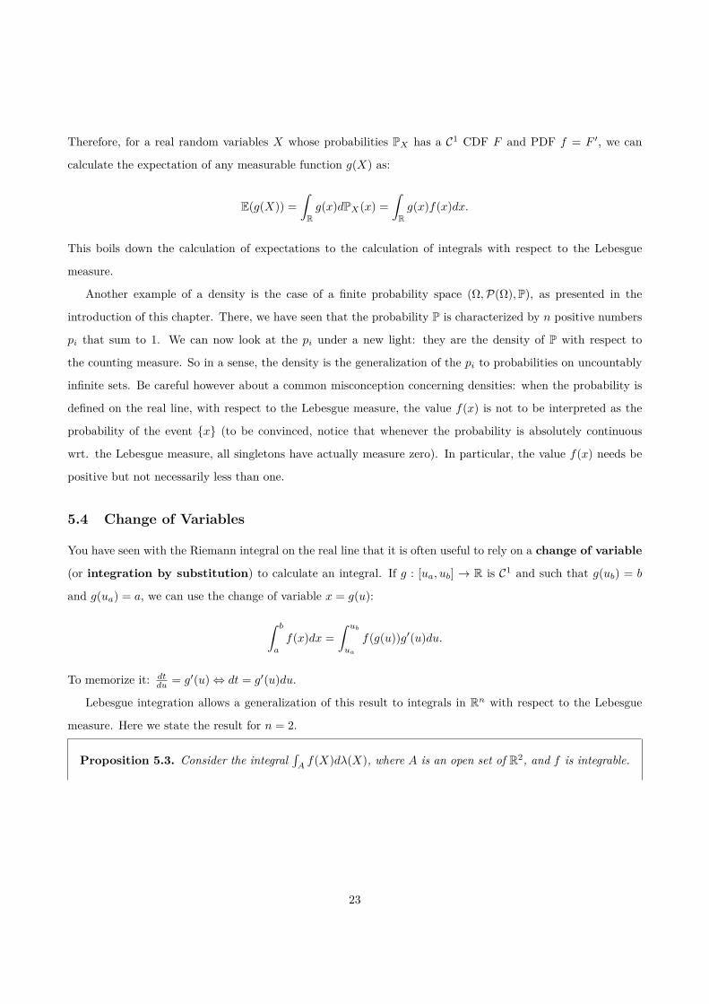
Therefore, for a real random variables X whose probabilities PX has a C1 CDF F and PDF f = F ′, we can

calculate the expectation of any measurable function g(X) as:

E(g(X)) =∫Rg(x)dPX(x) =

∫Rg(x)f(x)dx.

This boils down the calculation of expectations to the calculation of integrals with respect to the Lebesgue

measure.

Another example of a density is the case of a finite probability space (Ω,P(Ω),P), as presented in the

introduction of this chapter. There, we have seen that the probability P is characterized by n positive numbers

pi that sum to 1. We can now look at the pi under a new light: they are the density of P with respect to

the counting measure. So in a sense, the density is the generalization of the pi to probabilities on uncountably

infinite sets. Be careful however about a common misconception concerning densities: when the probability is

defined on the real line, with respect to the Lebesgue measure, the value f(x) is not to be interpreted as the

probability of the event x (to be convinced, notice that whenever the probability is absolutely continuous

wrt. the Lebesgue measure, all singletons have actually measure zero). In particular, the value f(x) needs be

positive but not necessarily less than one.

5.4 Change of Variables

You have seen with the Riemann integral on the real line that it is often useful to rely on a change of variable

(or integration by substitution) to calculate an integral. If g : [ua, ub] → R is C1 and such that g(ub) = b

and g(ua) = a, we can use the change of variable x = g(u):

∫ b

a

f(x)dx =∫ ub

ua

f(g(u))g′(u)du.

To memorize it: dtdu = g′(u)⇔ dt = g′(u)du.

Lebesgue integration allows a generalization of this result to integrals in Rn with respect to the Lebesgue

measure. Here we state the result for n = 2.

Proposition 5.3. Consider the integral∫Af(X)dλ(X), where A is an open set of R2, and f is integrable.

23

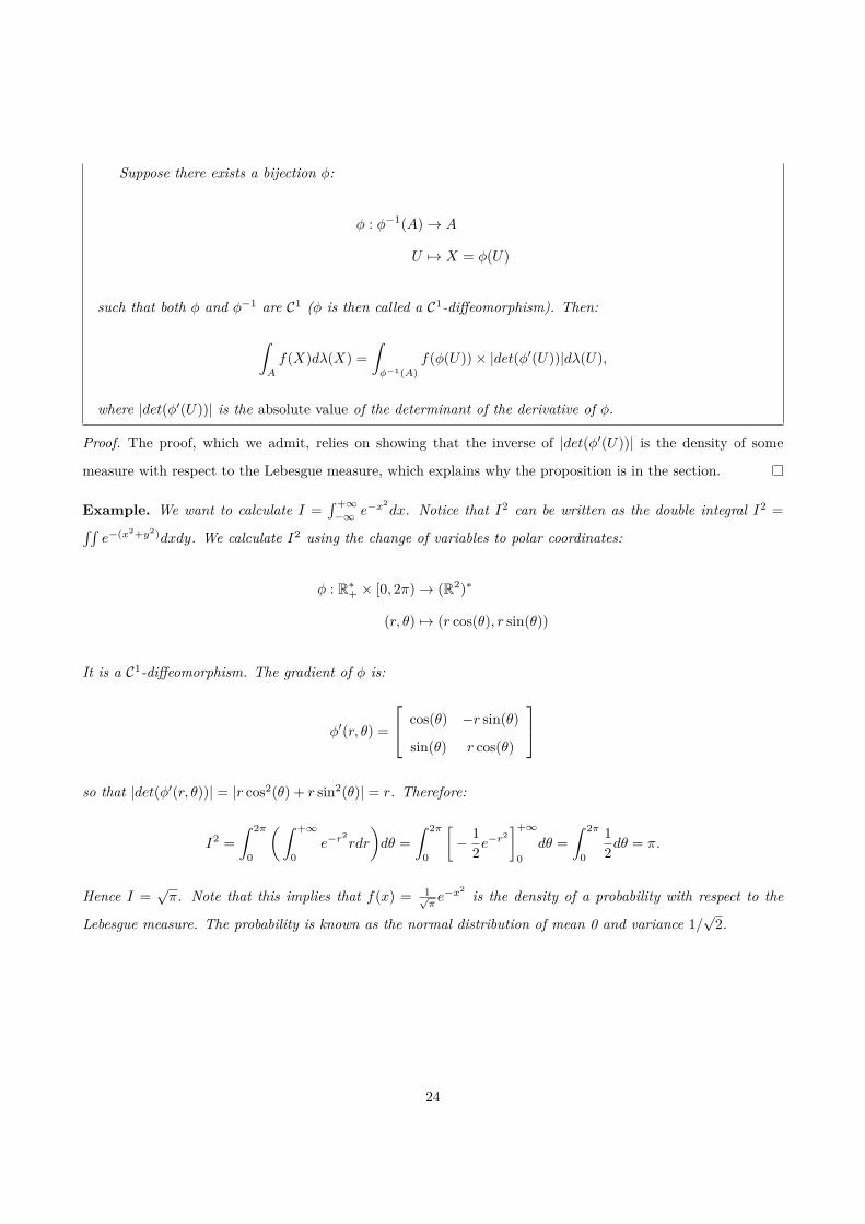
Suppose there exists a bijection φ:

φ : φ−1(A)→ A

U 7→ X = φ(U)

such that both φ and φ−1 are C1 (φ is then called a C1-diffeomorphism). Then:

∫A

f(X)dλ(X) =∫φ−1(A)

f(φ(U))× |det(φ′(U))|dλ(U),

where |det(φ′(U))| is the absolute value of the determinant of the derivative of φ.

Proof. The proof, which we admit, relies on showing that the inverse of |det(φ′(U))| is the density of some

measure with respect to the Lebesgue measure, which explains why the proposition is in the section.

Example. We want to calculate I =∫ +∞−∞ e−x

2dx. Notice that I2 can be written as the double integral I2 =∫∫

e−(x2+y2)dxdy. We calculate I2 using the change of variables to polar coordinates:

φ : R∗+ × [0, 2π)→ (R2)∗

(r, θ) 7→ (r cos(θ), r sin(θ))

It is a C1-diffeomorphism. The gradient of φ is:

φ′(r, θ) =

cos(θ) −r sin(θ)

sin(θ) r cos(θ)

so that |det(φ′(r, θ))| = |r cos2(θ) + r sin2(θ)| = r. Therefore:

I2 =∫ 2π

0

(∫ +∞

0e−r

2rdr

)dθ =

∫ 2π

0

[− 1

2e−r2]+∞

0dθ =

∫ 2π

0

12dθ = π.

Hence I =√π. Note that this implies that f(x) = 1√

πe−x

2 is the density of a probability with respect to the

Lebesgue measure. The probability is known as the normal distribution of mean 0 and variance 1/√

2.

24

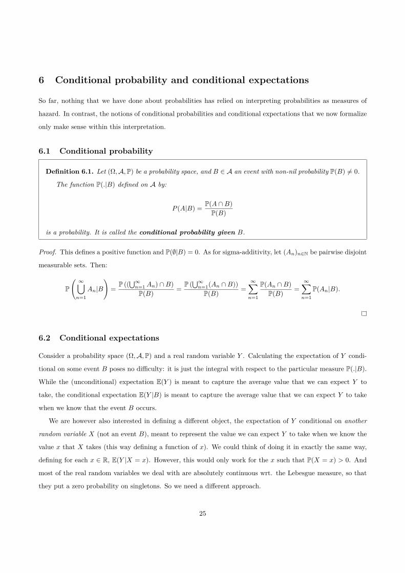
6 Conditional probability and conditional expectations

So far, nothing that we have done about probabilities has relied on interpreting probabilities as measures of

hazard. In contrast, the notions of conditional probabilities and conditional expectations that we now formalize

only make sense within this interpretation.

6.1 Conditional probability

Definition 6.1. Let (Ω,A,P) be a probability space, and B ∈ A an event with non-nil probability P(B) 6= 0.

The function P(.|B) defined on A by:

P (A|B) = P(A ∩B)P(B)

is a probability. It is called the conditional probability given B.

Proof. This defines a positive function and P(∅|B) = 0. As for sigma-additivity, let (An)n∈N be pairwise disjoint

measurable sets. Then:

P

( ∞⋃n=1

An|B

)=

P ((⋃∞n=1An) ∩B)P(B) =

P (⋃∞n=1(An ∩B))P(B) =

∞∑n=1

P(An ∩B)P(B) =

∞∑n=1

P(An|B).

6.2 Conditional expectations

Consider a probability space (Ω,A,P) and a real random variable Y . Calculating the expectation of Y condi-

tional on some event B poses no difficulty: it is just the integral with respect to the particular measure P(.|B).

While the (unconditional) expectation E(Y ) is meant to capture the average value that we can expect Y to

take, the conditional expectation E(Y |B) is meant to capture the average value that we can expect Y to take

when we know that the event B occurs.

We are however also interested in defining a different object, the expectation of Y conditional on another

random variable X (not an event B), meant to represent the value we can expect Y to take when we know the

value x that X takes (this way defining a function of x). We could think of doing it in exactly the same way,

defining for each x ∈ R, E(Y |X = x). However, this would only work for the x such that P(X = x) > 0. And

most of the real random variables we deal with are absolutely continuous wrt. the Lebesgue measure, so that

they put a zero probability on singletons. So we need a different approach.

25

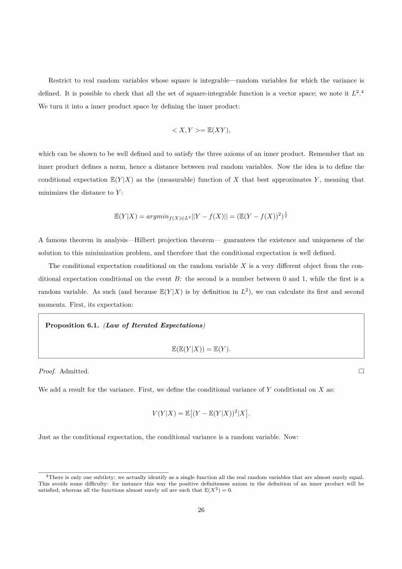
Restrict to real random variables whose square is integrable—random variables for which the variance is

defined. It is possible to check that all the set of square-integrable function is a vector space; we note it L2.4

We turn it into a inner product space by defining the inner product:

< X,Y >= E(XY ),

which can be shown to be well defined and to satisfy the three axioms of an inner product. Remember that an

inner product defines a norm, hence a distance between real random variables. Now the idea is to define the

conditional expectation E(Y |X) as the (measurable) function of X that best approximates Y , meaning that

minimizes the distance to Y :

E(Y |X) = argminf(X)∈L2 ||Y − f(X)|| = (E(Y − f(X))2) 12

A famous theorem in analysis—Hilbert projection theorem— guarantees the existence and uniqueness of the

solution to this minimization problem, and therefore that the conditional expectation is well defined.

The conditional expectation conditional on the random variable X is a very different object from the con-

ditional expectation conditional on the event B: the second is a number between 0 and 1, while the first is a

random variable. As such (and because E(Y |X) is by definition in L2), we can calculate its first and second

moments. First, its expectation:

Proposition 6.1. (Law of Iterated Expectations)

E(E(Y |X)) = E(Y ).

Proof. Admitted.

We add a result for the variance. First, we define the conditional variance of Y conditional on X as:

V (Y |X) = E[(Y − E(Y |X))2|X

].

Just as the conditional expectation, the conditional variance is a random variable. Now:

4There is only one subtlety: we actually identify as a single function all the real random variables that are almost surely equal.This avoids some difficulty: for instance this way the positive definiteness axiom in the definition of an inner product will besatisfied, whereas all the functions almost surely nil are such that E(X2) = 0.

26

Proposition 6.2.

V (E(Y |X)) = V (Y )− E(V (Y |X))

Proof. Admitted.

This decomposes the variance of Y between the variance of its conditional expectation and the expectation of its

conditional variance (this decomposition can be made for any random variable X). Note that the decomposition

implies V (Y ) ≥ V (E(Y |X)): we are less uncertain about Y when we know X.

27