
γλώσσες
Σελίδες
Νομικός

CSE598GRobert Collins
Mean-Shift Blob Trackingthrough Scale Space
Robert Collins, CVPR’03
CSE598GRobert Collins
Abstract
• Mean-shift tracking
• Choosing scale of kernel is an issue
• Scale-space feature selection provides inspiration
• Perform mean-shift with scale-space kernel to
optimize for blob location and scale
CSE598GRobert Collins
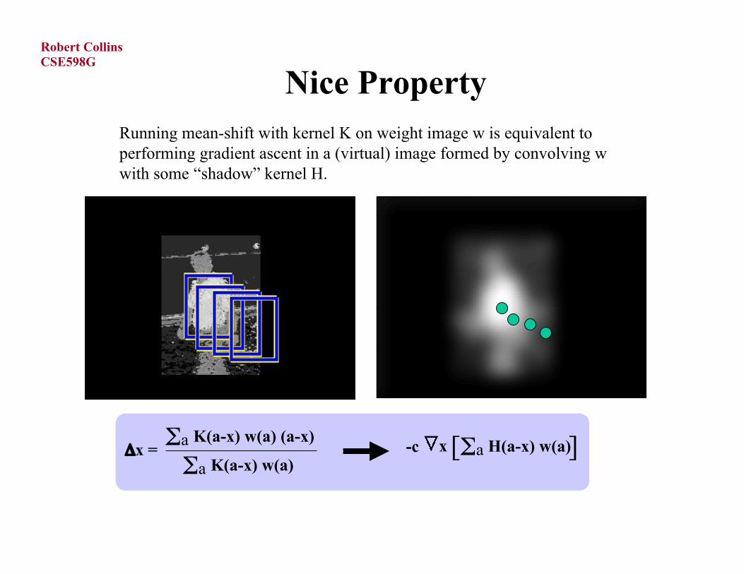
Nice Property
Δx = Σa K(a-x) w(a) (a-x)
Σa K(a-x) w(a)[Σa ]H(a-x) w(a)x
Running mean-shift with kernel K on weight image w is equivalent toperforming gradient ascent in a (virtual) image formed by convolving wwith some “shadow” kernel H.
-c
CSE598GRobert Collins
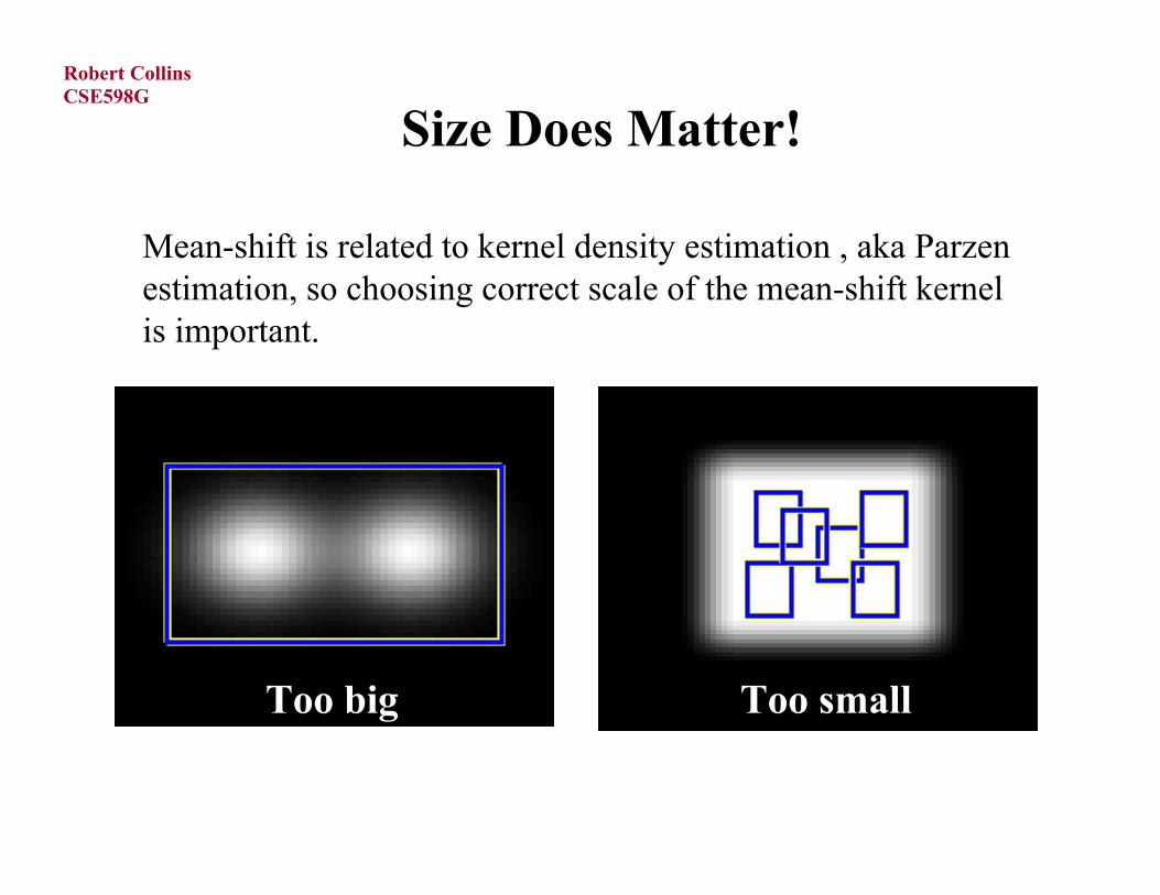
Size Does Matter!
Mean-shift is related to kernel density estimation , aka Parzenestimation, so choosing correct scale of the mean-shift kernel is important.
Too big Too small
CSE598GRobert Collins
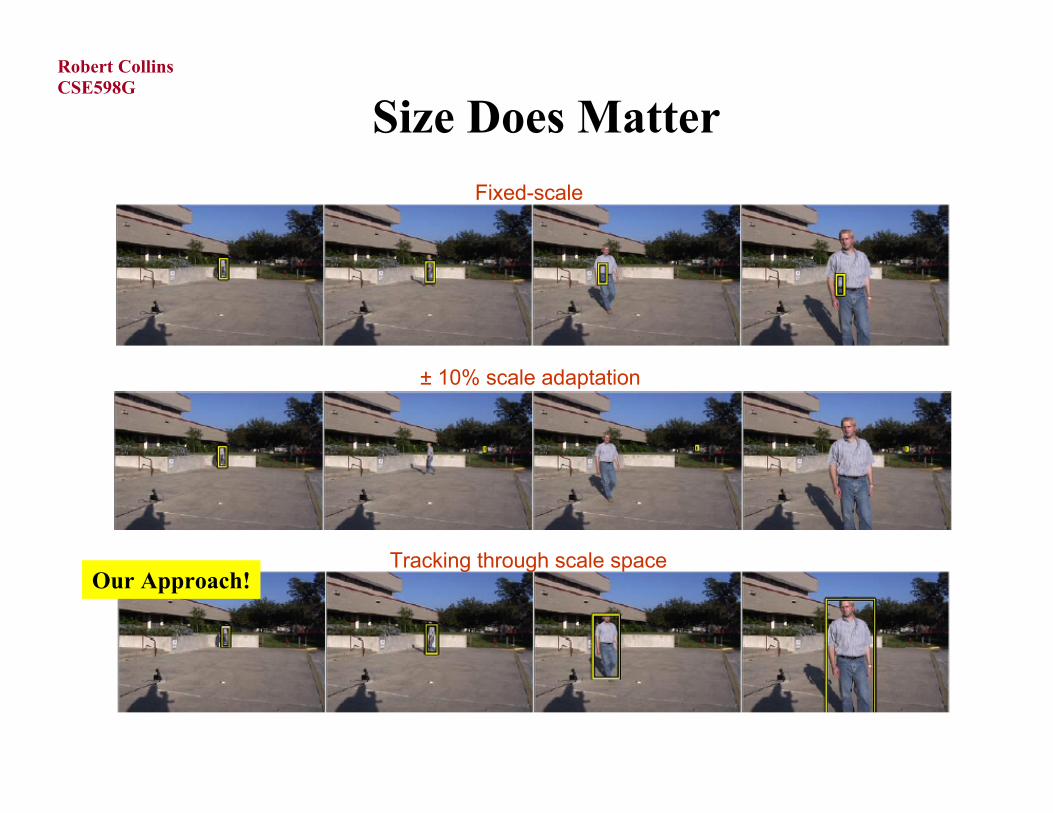
Size Does MatterFixed-scale
Tracking through scale space
± 10% scale adaptation
Our Approach!
CSE598GRobert Collins
Some Approaches to Size Selection
•Choose one scale and stick with it.
•Bradski’s CAMSHIFT tracker computes principal axes and scales from the secondmoment matrix of the blob. Assumes one blob, little clutter.
•CRM adapt window size by +/- 10% and evaluate using Battacharyya coefficient.Although this does stop the window from growing too big, it is not sufficient tokeep the window from shrinking too much.
•Comaniciu’s variable bandwidth methods. Computationally complex.
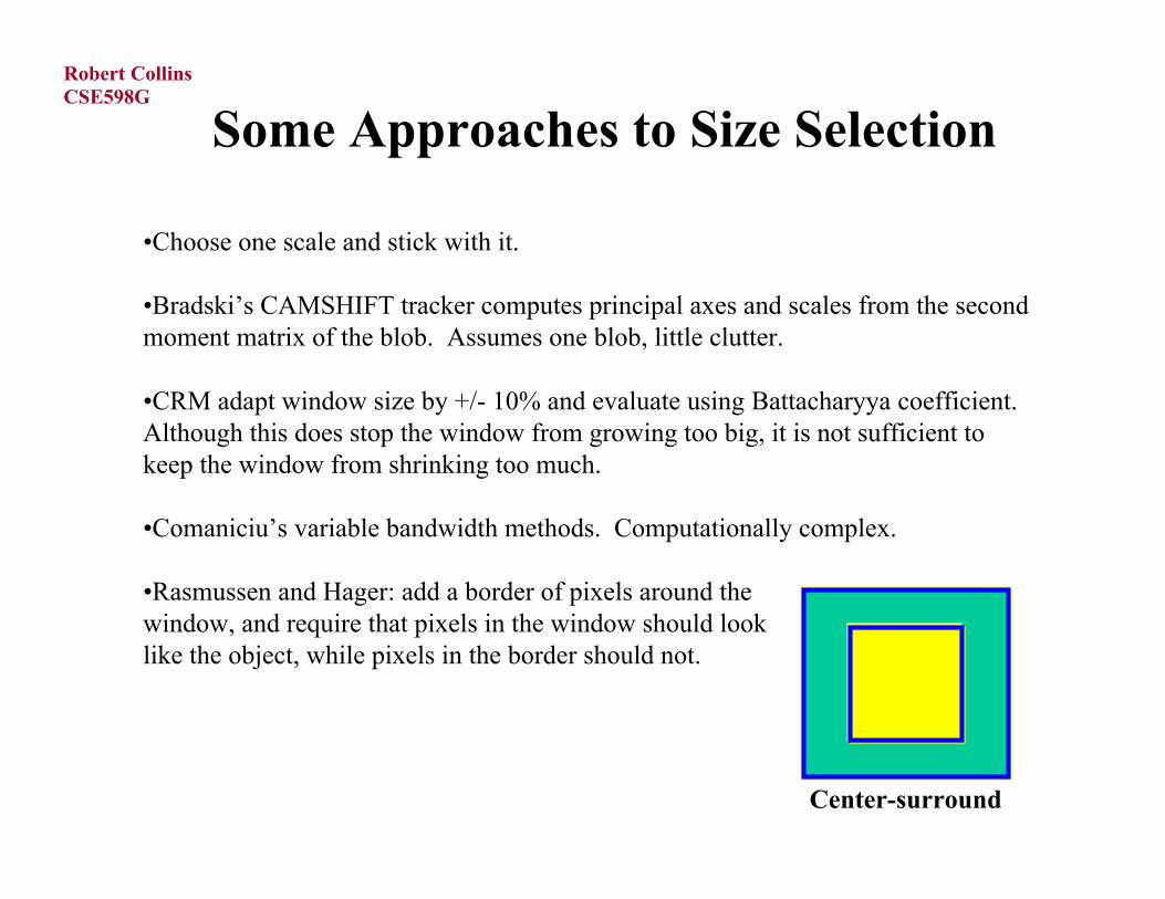
•Rasmussen and Hager: add a border of pixels around thewindow, and require that pixels in the window should looklike the object, while pixels in the border should not.
Center-surround
CSE598GRobert Collins
Scale-Space Theory
CSE598GRobert Collins
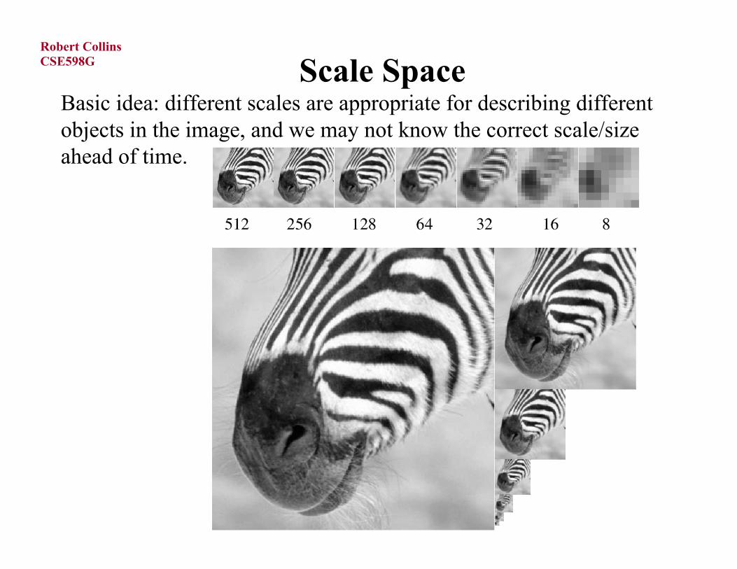
Basic idea: different scales are appropriate for describing differentobjects in the image, and we may not know the correct scale/sizeahead of time.
Scale Space
CSE598GRobert Collins
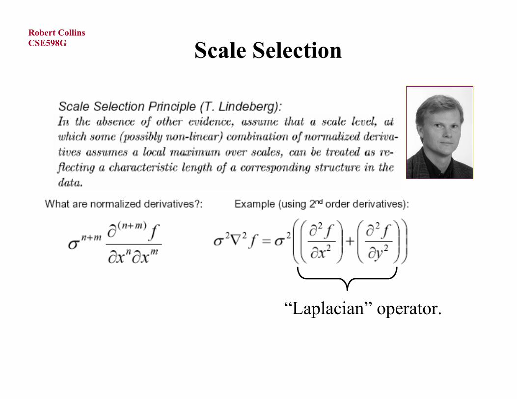
Scale Selection
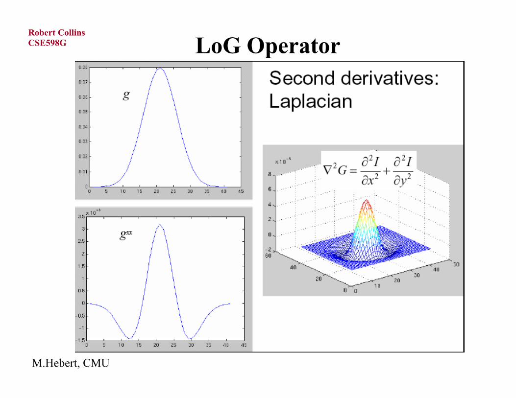
“Laplacian” operator.
CSE598GRobert Collins
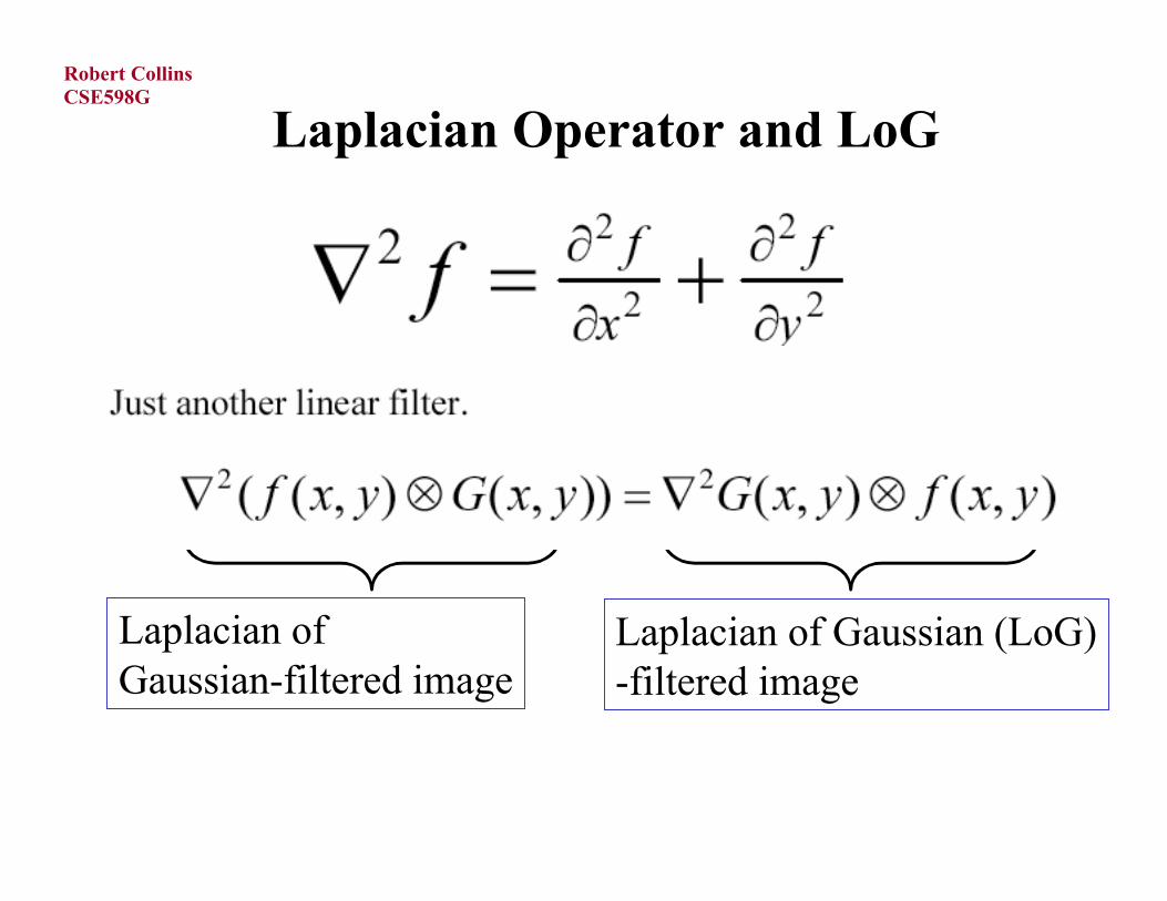
Laplacian Operator and LoG
Laplacian of Gaussian-filtered image
Laplacian of Gaussian (LoG)-filtered image
CSE598GRobert Collins
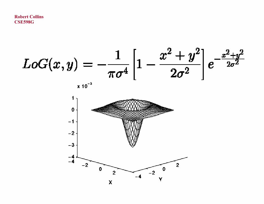
LoG Operator
M.Hebert, CMU
CSE598GRobert Collins
CSE598GRobert Collins
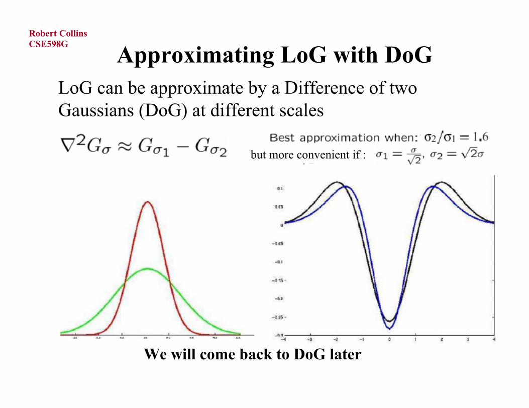
Approximating LoG with DoGLoG can be approximate by a Difference of two Gaussians (DoG) at different scales
We will come back to DoG later
but more convenient if :
CSE598GRobert Collins
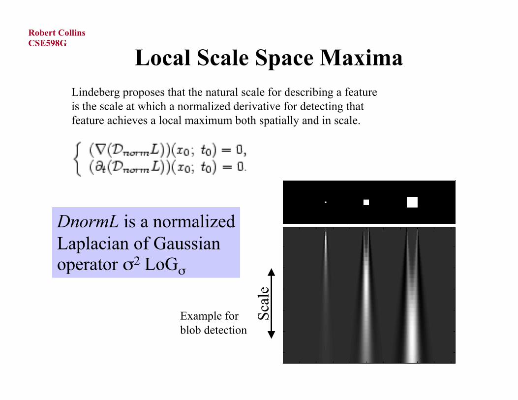
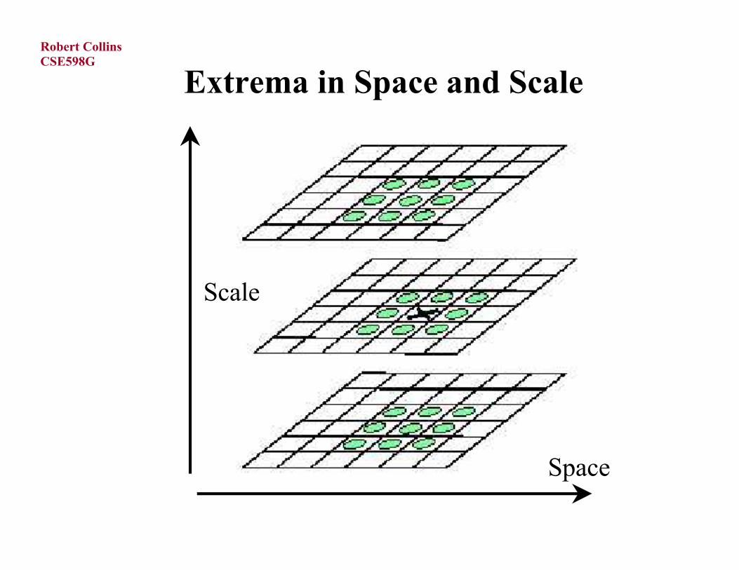
Local Scale Space MaximaLindeberg proposes that the natural scale for describing a featureis the scale at which a normalized derivative for detecting thatfeature achieves a local maximum both spatially and in scale.
Scal
e
Example forblob detection
DnormL is a normalizedLaplacian of Gaussianoperator σ2 LoGσ
CSE598GRobert Collins
Extrema in Space and Scale
Scale
Space
CSE598GRobert Collins
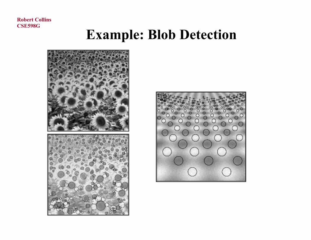
Example: Blob Detection
CSE598GRobert Collins
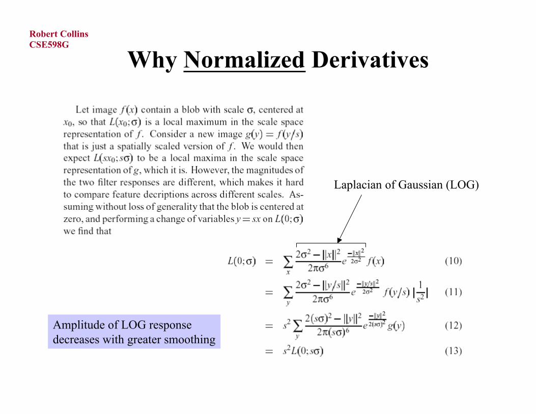
Why Normalized Derivatives
Laplacian of Gaussian (LOG)
Amplitude of LOG responsedecreases with greater smoothing
CSE598GRobert Collins
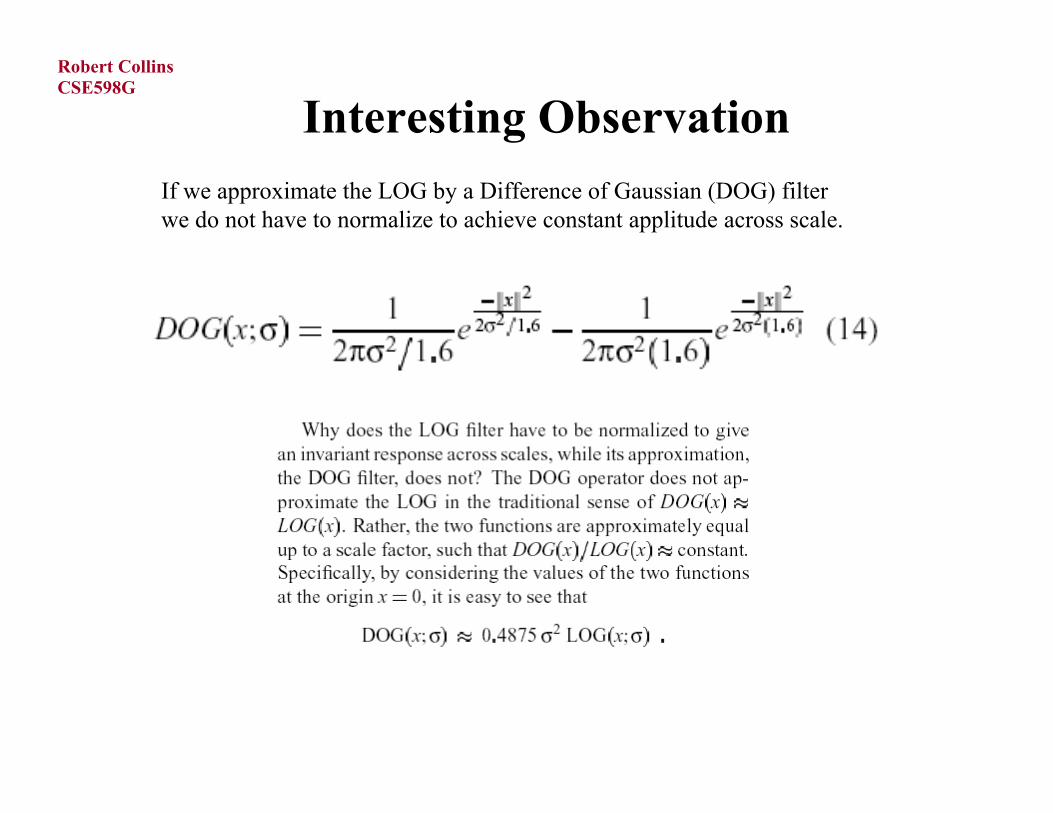
Interesting ObservationIf we approximate the LOG by a Difference of Gaussian (DOG) filterwe do not have to normalize to achieve constant applitude across scale.
CSE598GRobert Collins
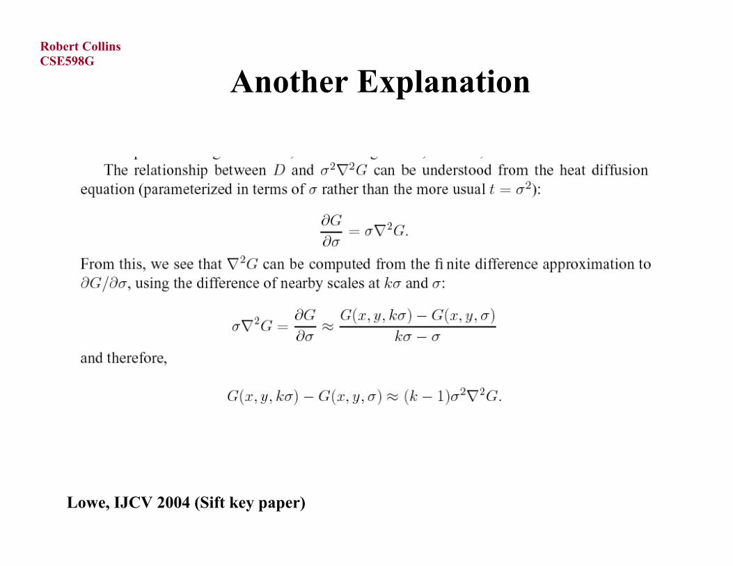
Another Explanation
Lowe, IJCV 2004 (Sift key paper)
CSE598GRobert Collins
Anyhow...
Scale space theory says we should look for modes ina DoG - filtered image volume. Let’s just think ofthe spatial dimensions for now
We want to look for modes in DoG-filtered image,meaning a weight image convolved with a DoG filter.
Insight: if we view DoG filter as a shadow kernel, wecould use mean-shift to find the modes. Of course, we’dhave to figure out what mean-shift kernel correspondsto a shadow kernel that is a DoG.
CSE598GRobert Collins
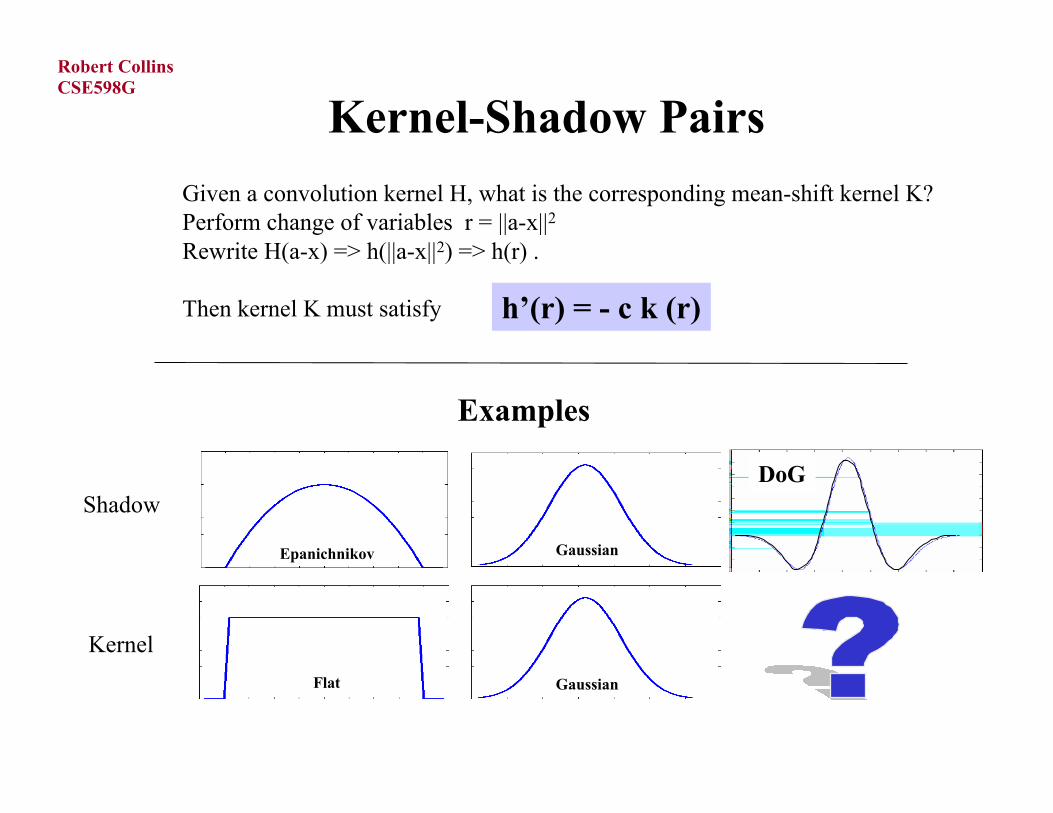
Kernel-Shadow Pairs
h’(r) = - c k (r)
Given a convolution kernel H, what is the corresponding mean-shift kernel K?Perform change of variables r = ||a-x||2 Rewrite H(a-x) => h(||a-x||2) => h(r) .
Then kernel K must satisfy
Examples
Shadow
Kernel
Epanichnikov
Flat
Gaussian
Gaussian
DoG
CSE598GRobert Collins
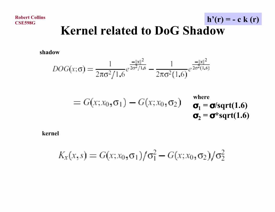
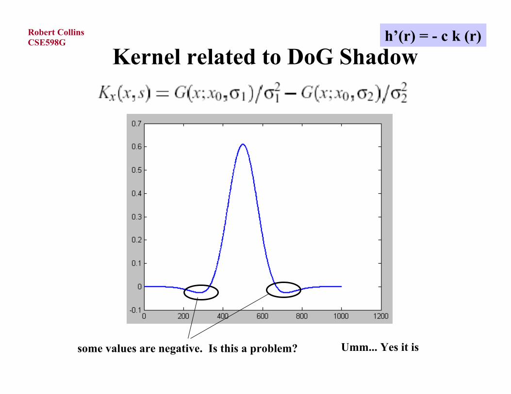
Kernel related to DoG Shadow
shadow
kernel
h’(r) = - c k (r)
where
σ1 = σ/sqrt(1.6)σ2 = σ*sqrt(1.6)
CSE598GRobert Collins
Kernel related to DoG Shadowh’(r) = - c k (r)
some values are negative. Is this a problem? Umm... Yes it is

CSE598GRobert Collins
Dealing with Negative Weights
CSE598GRobert Collins
Show little demo with neg weights
mean-shift will sometimes converge to a valley rather than a peak.
The behavior is sometimes even stranger than that (step size becomesway too big and you end up in another part of the function).
CSE598GRobert Collins
Why we might want negative weights
iii dmw /=
i
ii d
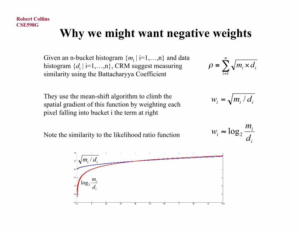
mw 2log≈
Given an n-bucket histogram {mi | i=1,…,n} and datahistogram {di | i=1,…,n}, CRM suggest measuringsimilarity using the Battacharyya Coefficient
∑=
×≡n
iii dm
1
ρ
They use the mean-shift algorithm to climb thespatial gradient of this function by weighting eachpixel falling into bucket i the term at right
Note the similarity to the likelihood ratio function
i
i
d
m2log
ii dm /
CSE598GRobert Collins
Why we might want negative weights
i
ii d
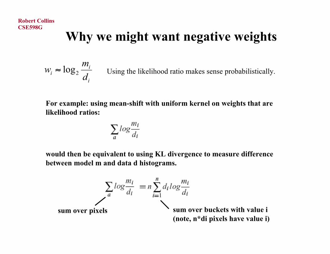
mw 2log≈ Using the likelihood ratio makes sense probabilistically.
For example: using mean-shift with uniform kernel on weights that arelikelihood ratios:
would then be equivalent to using KL divergence to measure differencebetween model m and data d histograms.
sum over pixels sum over buckets with value i(note, n*di pixels have value i)
CSE598GRobert Collins
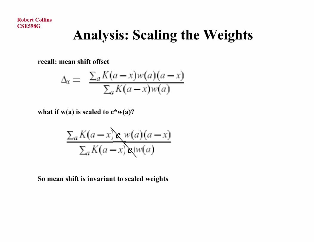
Analysis: Scaling the Weights
recall: mean shift offset
what if w(a) is scaled to c*w(a)?
cc
So mean shift is invariant to scaled weights
CSE598GRobert Collins
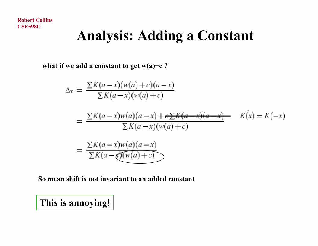
Analysis: Adding a Constant
what if we add a constant to get w(a)+c ?
So mean shift is not invariant to an added constant
This is annoying!
CSE598GRobert Collins
Adding a Constant
result: It isn’t a good idea to just add a large positive number toour weights to make sure they stay positive.
show little demo again, adding a constant.
CSE598GRobert Collins
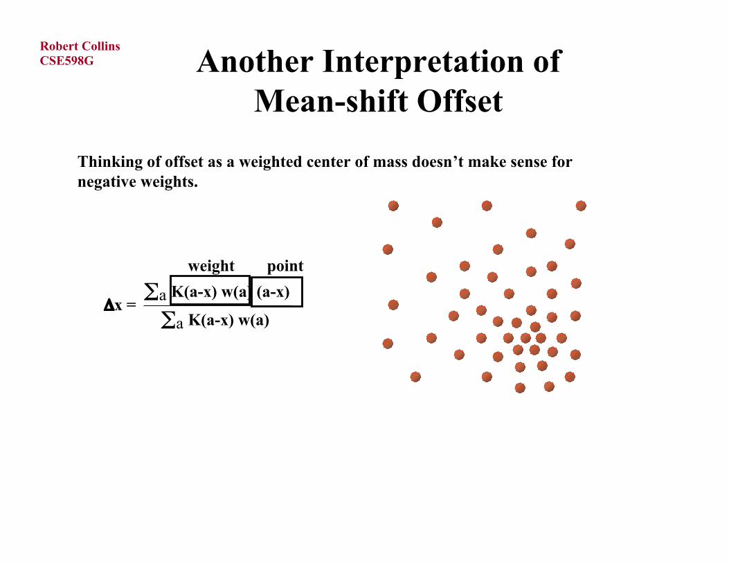
Another Interpretation ofMean-shift Offset
Thinking of offset as a weighted center of mass doesn’t make sense fornegative weights.
Δx = Σa K(a-x) w(a) (a-x)
Σa K(a-x) w(a)
pointweight
CSE598GRobert Collins
Another Interpretation ofMean-shift Offset
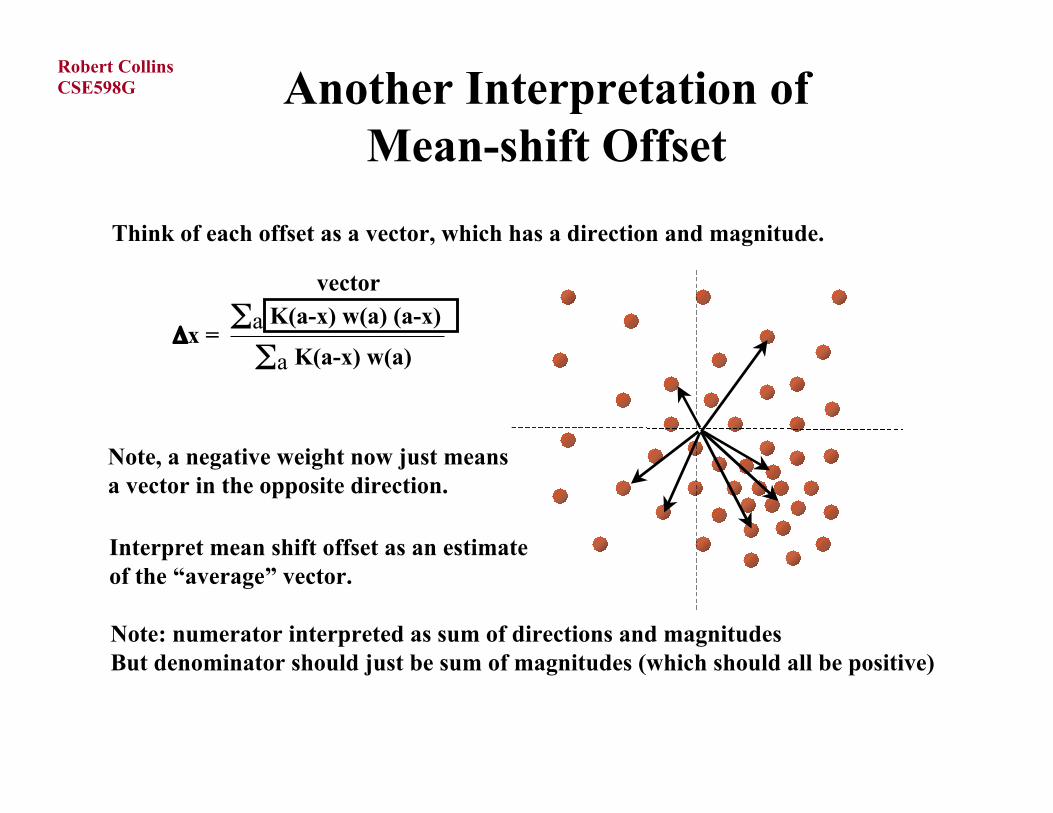
Think of each offset as a vector, which has a direction and magnitude.
Δx = Σa K(a-x) w(a) (a-x)
Σa K(a-x) w(a)
Interpret mean shift offset as an estimateof the “average” vector.
vector
Note, a negative weight now just meansa vector in the opposite direction.
Note: numerator interpreted as sum of directions and magnitudesBut denominator should just be sum of magnitudes (which should all be positive)
CSE598GRobert Collins
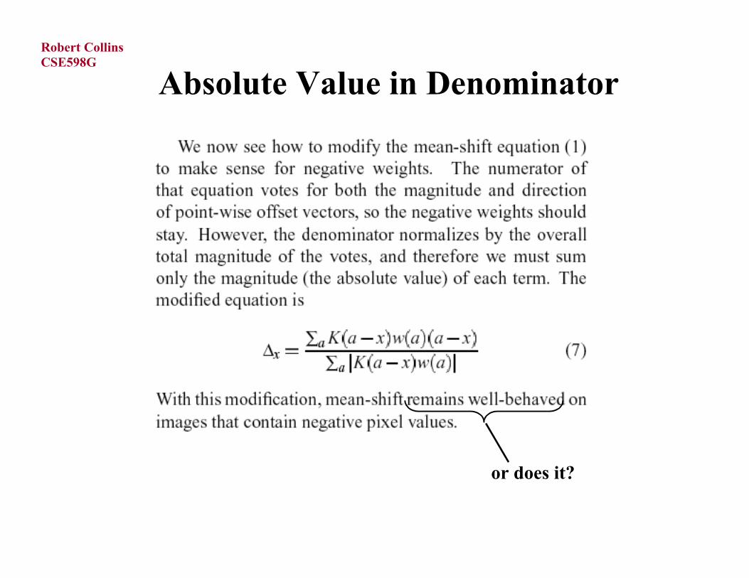
Absolute Value in Denominator
or does it?
CSE598GRobert Collins
back to the demo
There can be oscillations when there are negative weights.I’m not sure what to do about that.
CSE598GRobert Collins
Outline of Scale-Space Mean Shift
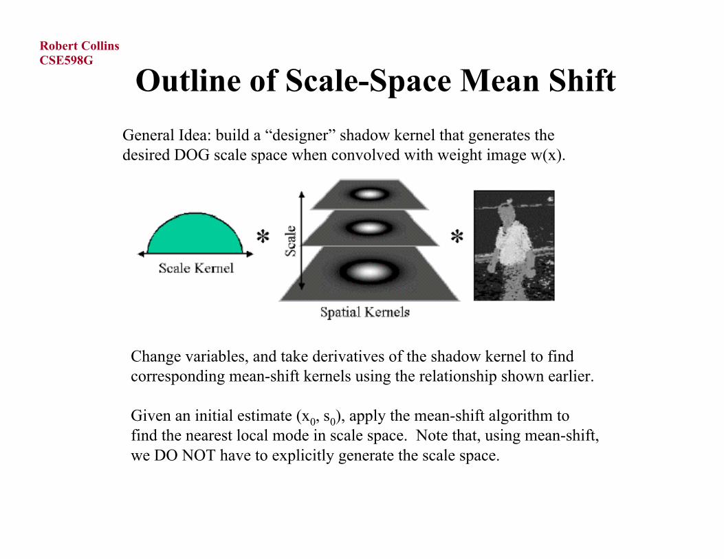
General Idea: build a “designer” shadow kernel that generates thedesired DOG scale space when convolved with weight image w(x).
Change variables, and take derivatives of the shadow kernel to findcorresponding mean-shift kernels using the relationship shown earlier.
Given an initial estimate (x0, s0), apply the mean-shift algorithm to find the nearest local mode in scale space. Note that, using mean-shift,we DO NOT have to explicitly generate the scale space.
CSE598GRobert Collins
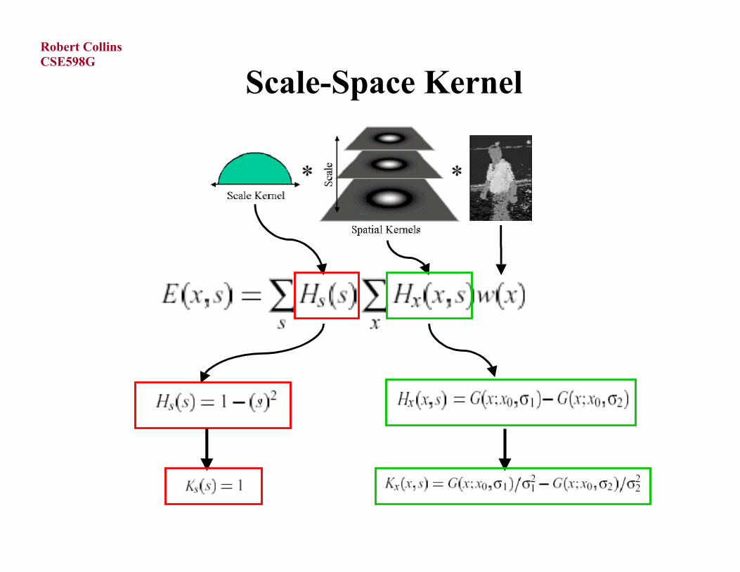
Scale-Space Kernel
CSE598GRobert Collins
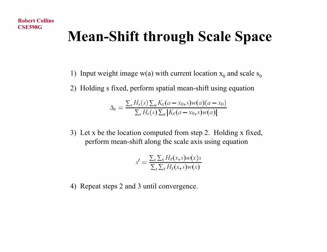
Mean-Shift through Scale Space
1) Input weight image w(a) with current location x0 and scale s0
2) Holding s fixed, perform spatial mean-shift using equation
3) Let x be the location computed from step 2. Holding x fixed,perform mean-shift along the scale axis using equation
4) Repeat steps 2 and 3 until convergence.
CSE598GRobert Collins
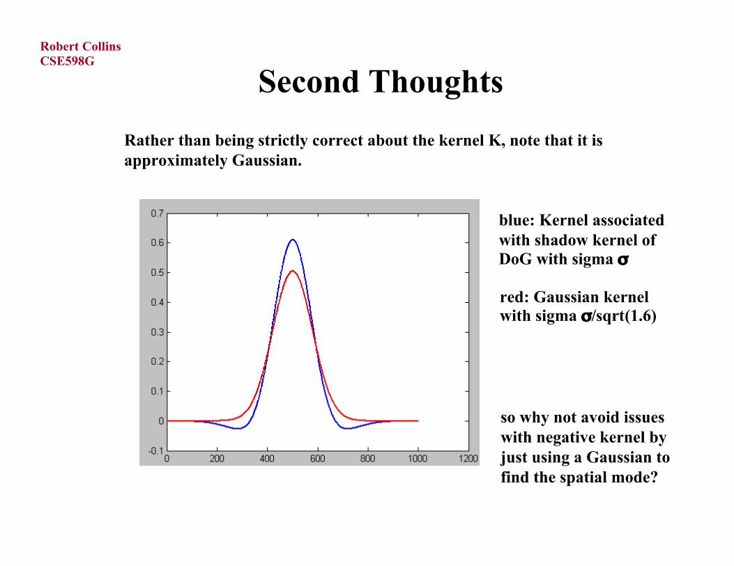
Second Thoughts
Rather than being strictly correct about the kernel K, note that it isapproximately Gaussian.
blue: Kernel associatedwith shadow kernel ofDoG with sigma σ
red: Gaussian kernelwith sigma σ/sqrt(1.6)
so why not avoid issueswith negative kernel byjust using a Gaussian tofind the spatial mode?
CSE598GRobert Collins
scaledemo.m
interleave Gaussian spatial mode finding with 1D DoG mode finding.
CSE598GRobert Collins
Summary
• Mean-shift tracking
• Choosing scale of kernel is an issue
• Scale-space feature selection provides inspiration
• Perform mean-shift with scale-space kernel to optimize for blob
location and scale
Contributions
• Natural mechanism for choosing scale WITHIN mean-shift framework
• Building “designer” kernels for efficient hill-climbing on (implicitly-
defined) convolution surfaces
Top Related