BV SOLUTIONS CONSTRUCTED BY EPSILON-NEIGHBORHOOD METHOD

Mach Nguyet Minh

Dipartimento di Matematica

Universita di Pisa

Largo Bruno Pontecorvo 5, 56127 Pisa, Italy

Abstract. We study a certain class of weak solutions to rate-independent systems, which is constructed

by using the local minimality in a small neighborhood of order ε and then taking the limit ε → 0. We show

that the resulting solution satisfies both the weak local stability and the new energy-dissipation balance,similarly to the BV solutions constructed by vanishing viscosity introduced recently by Mielke, Rossi and

Savare [19, 20, 21].

1. Introduction

A rate-independent system is a specific case of quasistatic systems. It is time-dependent but its behavioris slow enough that the inertial effects can be ignored and the systems are affected only by external loadings.Some specific rate-independent systems were studied by many authors including Francfort, Marigo, Larsen,Dal Maso and Lazzaroni on brittle fractures [9, 8, 11, 6], Dal Maso, DeSimone and Solombrino on theCam-Clay model [5], Dal Maso, DeSimone, Mora, Morini on plasticity with softening [3, 4], Mielke on elasto-plasticity [13, 14], Mielke, Theil and Levitas on shape-memory alloys [22, 23, 24], Muller, Schmid and Mielkeon super-conductivity [26, 29], and Alberti and DeSimone on capillary drops [1]. We refer to the surveys[16, 15, 17, 18] by Mielke for the study in abstract setting as well as for further references.

In this work, we consider a finite-dimensional normed vector space X, an evolution u : [0, T ]→ X subjectto a force defined by an energy functional E : [0, T ] ×X → [0,+∞) which is of class C1, and a dissipationfunction Ψ(x) which is convex, non-degenerate and positively 1-homogeneous. Given an initial positionx0 ∈ X which is a local minimizer for the functional x 7→ E (0, x) + Ψ(x− x0), we say that u is a solution tothe rate-independent system (E ,Ψ, x0) if u(0) = x0 and the following inclusion holds true,

0 ∈ ∂Ψ(u(t)) +DxE (t, u(t)) in X∗, for a.e. t ∈ (0, T ),(1)

where X∗ denotes the dual space of X, ∂Ψ is the subdifferential of Ψ and DxE is the differential of E w.r.t.the spatial variable x.

In general, strong solutions to (1) may not exist [30]. Hence, the question on defining some weak solutionsarises naturally.

A widely-used weak solution is the energetic solution, which was first introduced by Mielke and Theil [22](see [23, 12, 10, 16] for further studies). A function u : [0, T ] → X is called an energetic solution to therate-independent system (E ,Ψ, x0), if it satisfies

(i) the initial condition u(0) = x0;(ii) the global stability that for (t, x) ∈ [0, T ]×X,

E (t, u(t)) ≤ E (t, x) + Ψ(x− u(t));(2)

(iii) the energy-dissipation balance that for all 0 ≤ t1 ≤ t2 ≤ T ,

E (t2, u(t2))− E (t1, u(t1)) =

∫ t2

t1

∂tE (s, u(s)) ds−DissΨ(u; [t1, t2]).(3)

Here DissΨ is the usual total variation induced by Ψ(·)

DissΨ(u(t); [t1, t2]) := sup

{N∑i=1

Ψ(u(si)− u(si−1)) | N ∈ N, t1 = s0 < s1 < · · · < sN = t2

}.

Date: June 20, 2014.

1991 Mathematics Subject Classification. Primary: 49M99; Secondary: 49J20.

Key words and phrases. Rate-independent systems, BV solutions, local minimizers, energy-dissipation balance.

1

2 MACH NGUYET MINH

Notice that when the energy functional is not convex, the global minimality (2) makes the energeticsolutions jump sooner than they should, and hence fail to describe the related physical phenomena (seeExamples 2 below). Therefore, some weak solutions based on local minimality are of interests.

Recently, an elegant weak solution based on vanishing viscosity method was introduced by Mielke, Rossiand Savare [19, 20, 21]. Their idea is to add a small viscosity term to the dissipation functional Ψ. Thisresults in a new dissipation functional Ψε, e.g. Ψε(x) = Ψ(x) + ε

2‖x‖2, which has super-linear growth at

infinity and converges to Ψ in an appropriate sense as ε tends to zero. They showed that the modified system(E ,Ψε, x0) admits a solution uε. The limit u of a subsequence uε as ε → 0, called BV solution, enjoys thefollowing properties

(i) the initial condition u(0) = x0;(ii) the weak local stability that for all t ∈ [0, T ]\J ,

−DxE (t, u(t)) ∈ ∂Ψ(0);(4)

(iii) the new energy-dissipation balance that for all 0 ≤ t1 ≤ t2 ≤ T ,

E (t2, u(t2))− E (t1, u(t1)) =

∫ t2

t1

∂tE (s, u(s)) ds−Dissnew(u; [t1, t2]).(5)

Here J is the jump set of u on [0, T ]

J := {t ∈ [0, T ] | u(·) is not continuous at t},∂Ψ(0) is the subdifferential of Ψ at 0, 〈·, ·〉 is the dual pairing between X∗ and X

∂Ψ(0) := {η ∈ X∗ | 〈η, v〉 ≤ Ψ(v) ∀v ∈ X},and the new dissipation is defined by

Dissnew(u; [t1, t2]) := DissΨ(u; [t1, t2]) +∑

t∈J∩(t1,t2)

(∆new(t;u(t−), u(t)) + ∆new(t;u(t), u(t+))

)+∆new(t1;u(t1), u(t+1 )) + ∆new(t2;u(t−2 ), u(t2))

−∑

t∈J∩(t1,t2)

(Ψ(u(t)− u(t−)) + Ψ(u(t+)− u(t))

)−Ψ(u(t+1 )− u(t1))−Ψ(u(t2)− u(t−2 )),

where ∆new(t; a, b) depends also on the energy functional E , the dissipation Ψ and the viscous norm ‖ · ‖

∆new(t; a, b) = inf

{∫ 1

0

(Ψ(γ(s)) + ‖γ(s)‖ · inf

z∈∂Ψ(0)‖DxE (t, γ(s)) + z‖∗

)ds | γ ∈ AC([0, 1];X), γ(0) = a, γ(1) = b

}.

Here the dual norm of ‖ · ‖ is defined by ‖η‖∗ = supv∈X\{0}|〈η,v〉|‖v‖ for all η ∈ X∗.

The new energy-dissipation balance is a deeply insight observation, which contains the information at thejump points. Indeed, it was shown in [20, 21] that if the BV solution u jumps at time t, there exists anabsolutely continuous path γ : [0, 1]→ X, which called an optimal transition between u(t−) and u(t+), suchthat

(i) γ(0) = u(t−), γ(1) = u(t+), and there exists s ∈ [0, 1] such that γ(s) = u(t);(ii) for all s ∈ [0, 1],−DxE (t, γ(s)) stays outside the set ∂Ψ(0) (if γ is of viscous type), or on the boundary

of ∂Ψ(0) (if γ is of sliding type);

(iii) E (t, u(t−))− E (t, u(t+)) =∫ 1

0

(Ψ(γ(s)) + ‖γ(s)‖ · infz∈∂Ψ(0) ‖DxE (t, γ(s)) + z‖∗

)ds.

As we can see from the definition, BV solutions constructed by vanishing viscosity depend also on theviscosity. Usually, the viscosity arises naturally from physical models.

To deal with local minimizers but with a totally different approach, Larsen [11] proposed the ε-stabilitysolution in the context of fracture mechanics. The idea is to choose minimizers among all ε-accessible statesw.r.t. the discretized solution at previous time-step. A state v is called ε-accessible w.r.t. state z if the totalenergy at v is lower than the total energy at z, and there is a continuous path connecting z to v such thatalong this path the total energy never increases by more than ε. By this way, the limit u(t) when passingfrom discrete to continuous time satisfies the so-called ε-stability: u(t) is ε-stable at every time t, i.e. thereis no ε-accessible state w.r.t. u(t). A similar version of optimal transition is obtained at jump points: ifsolution jumps at time t, there exists a continuous path connecting u(t−) to u(t+) such that along this path,the total energy increases no more than ε. The energy-dissipation upper bound is proved for fixed ε > 0.The energy-dissipation equality is obtained if the solution has only jumps of size less than ε.

BV SOLUTIONS VIA EPSILON-NEIGHBORHOOD METHOD 3

In this work, we shall discuss one more way to deal with local minimizers. The idea is more likely tothe viscosity method of Mielke-Rossi-Savare in [19, 20, 21], but instead of adding a small viscosity into thedissipation, we consider the minimization problem (2) in a small neighborhood of order ε. Passing fromdiscrete to continuous time, we obtain a limit xε(·). Then taking ε→ 0, we get a solution u(·). The epsilon-neighborhood approach was first suggested in [14, Section 6] for one-dimensional case when ε is chosenproportional to the square root of the time-step and the weak local stability was then obtained in [7].

Roughly speaking, epsilon-neighborhood method is a special case of vanishing viscosity approach whenviscosity term is chosen as follows

Ψ0(v) :=

{0 if |v| ≤ 1,

+∞ if |v| > 1.

However, this method was not discussed in [20, 21] since the viscosity there is required to be finite (see [20,Section 2.3] and [21, Section 2.1] for further discussions).

In this article, we shall show that the BV solution constructed by epsilon-neighborhood method u(·)satisfies both the weak local stability and the new energy-dissipation balance, i.e. it satisfies the definitionof BV solutions introduced by Mielke, Rossi and Savare [19, 20, 21]. Similar to BV solutions constructedby vanishing viscosity, BV solutions constructed by epsilon-neighborhood method also depend on the normthat defines the “neighborhood”. In Example 2 below, we shall give a comparison between different notionsof weak solutions, i.e. energetic solutions, BV solutions constructed by vanishing viscosity, BV solutionsconstructed by epsilon-neighborhood method as well as the solutions constructed by the method in [7]. Fora detailed discussion on the different notions of weak solutions, we refer to the papers [18, 28, 31, 25].

Acknowledgments. I am indebted to Professor Giovanni Alberti for proposing to me the problem andgiving many helpful discussions. I warmly thank Professor Riccarda Rossi, Li-Chang Hung and Tran Minh-Binh for their helpful comments and remarks. I really appreciate the three referees for many enlightening andinsightful remarks and helpful suggestions and corrections. This work has been partially supported by thePRIN 2008 grant “Optimal mass transportation, Geometric and Functional Inequalities and Applications”and the FP7-REGPOT-2009-1 project “Archimedes Center for Modeling, Analysis and Computation”.

2. Main results

For simplicity, we shall consider the case when X = Rd and the unit ball of the norm ‖·‖ which defines theneighborhood has C1-boundary. In addition, we assume that the energy functional E (t, x) : [0, T ] × Rd →[0,∞) satisfies the following technical assumption: there exists λ = λ(E ) such that

|∂tE (s, x)| ≤ λE (s, x) for all (s, x) ∈ [0, T ]×Rd.(6)

Remark. The condition (6) was proposed in [18]. Together with Gronwall’s inequality, (6) implies that

E (r, x) ≤ E (s, x) eλ|r−s|, |∂tE (r, x)| ≤ λE (s, x) eλ|r−s|(7)

for any r, s in [0, T ].

Definition (Construction of discretized solutions). Let ε > 0, τ > 0 and let N ∈ N satisfy T ∈ [τN, τ(N+1)).We define a sequence {xε,τ}Ni=0 by xε,τ0 = x0 (initial position) and

xε,τi ∈ argmin{E (ti, x) + Ψ(x− xε,τi−1) | ‖x− xε,τi−1‖ ≤ ε} for every i ∈ {1, . . . , N}.(8)

The discretized solution xε,τ (·) is then constructed by interpolation

xε,τ (t) := xε,τi−1 for every t ∈ [ti−1, ti), i ∈ {1, . . . , N}.

Our main result is as follows.

Theorem 1 (BV solutions constructed by epsilon-neighborhood method). Let E : [0, T ]×Rd → [0,+∞) beof class C1 and satisfy (6). The dissipation functional Ψ : Rd → [0,∞) is assumed to be convex, positively1-homogeneous and satisfy Ψ(v) > 0 for all v ∈ Rd\{0}. Given an initial datum x0 ∈ Rd which is a localminimizer of the functional x 7→ E (0, x) + Ψ(x− x0). Then we have the following properties.

(i) (Discretized solution) For any ε > 0 and τ > 0, there exists a discretized solution t 7→ xε,τ (·) asdescribed above.

(ii) (Epsilon-neighborhood solution) For any fixed ε > 0, there exists a subsequence τn → 0 such thatxε,τn(·) converges pointwise to some limit xε(·). Moreover,

4 MACH NGUYET MINH

• (Epsilon local stability) If xε(·) is right-continuous at t, namely limt′→t+ xε(t′) = xε(t), then xε(t)

satisfies the epsilon local stability

E (t, xε(t)) ≤ E (t, x) + Ψ(x− xε(t)) for all ‖x− xε(t)‖ ≤ ε;

• (Energy-dissipation inequalities) We have DissΨ(xε; [0, T ]) ≤ C (independent of ε), ∂tE (·, xε(·)) ∈L1(0, T ) and for all 0 ≤ s ≤ t ≤ T ,

−Dissnew(xε; [s, t]) ≤ E (t, xε(t))− E (s, xε(s))−∫ t

s

∂tE (r, xε(r)) dr ≤ −DissΨ(xε; [s, t]).

(iii) (BV solutions constructed by epsilon-neighborhood) There exists a subsequence εn → 0 such that xεn

converges pointwise to some BV function u. Furthermore, the function u satisfies• (Weak local stability) If t 7→ u(t) is continuous at t, then

−∇xE (t, u(t)) ∈ ∂Ψ(0);

• (New energy-dissipation balance) For all 0 ≤ s ≤ t ≤ T , one has

E (t, u(t))− E (s, u(s)) =

∫ t

s

∂tE (r, u(r)) dr −Dissnew(u; [s, t]).

An explicit example is given below (a detail explanation can be found in Appendix).

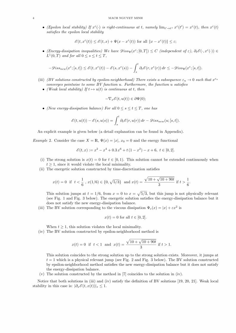
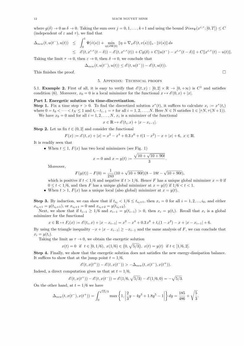
Example 2. Consider the case X = R, Ψ(x) = |x|, x0 = 0 and the energy functional

E (t, x) := x2 − x4 + 0.3x6 + t (1− x2)− x+ 6, t ∈ [0, 2].

(i) The strong solution is x(t) = 0 for t ∈ [0, 1). This solution cannot be extended continuously whent ≥ 1, since it would violate the local minimality.

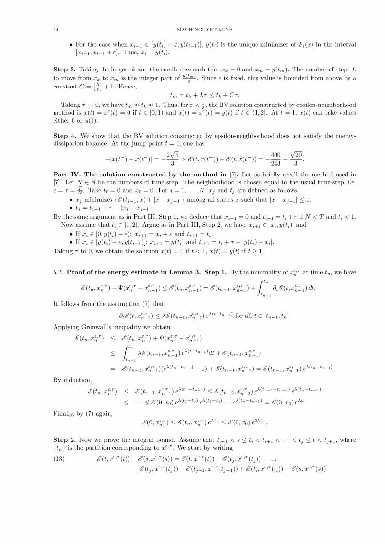
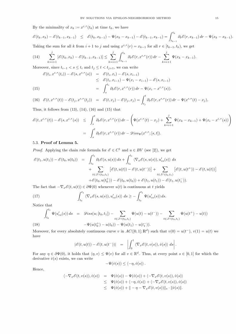
(ii) The energetic solution constructed by time-discretization satisfies

x(t) = 0 if t <1

6, x(1/6) ∈ {0,

√5/3} and x(t) =

√10 +

√10 + 90t

3if t >

1

6.

This solution jumps at t = 1/6, from x = 0 to x =√

5/3, but this jump is not physically relevant(see Fig. 1 and Fig. 3 below). The energetic solution satisfies the energy-dissipation balance but itdoes not satisfy the new energy-dissipation balance.

(iii) The BV solution corresponding to the viscous dissipation Ψε(x) = |x|+ εx2 is

x(t) = 0 for all t ∈ [0, 2].

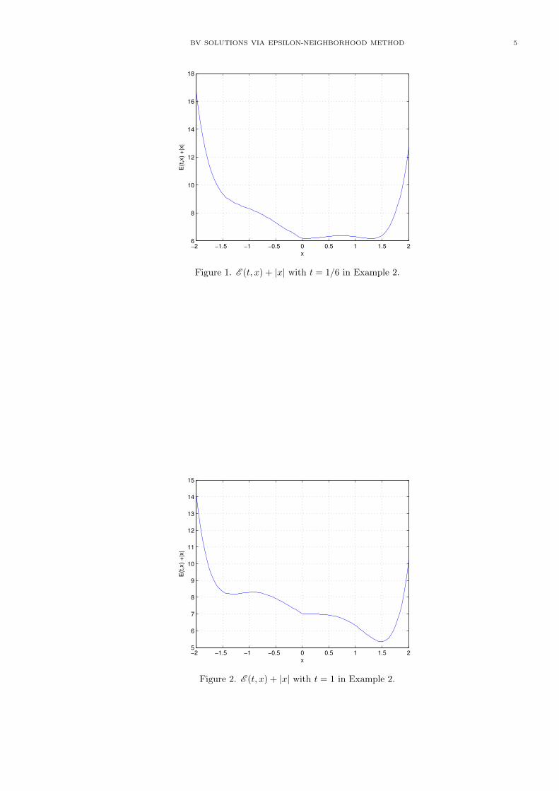
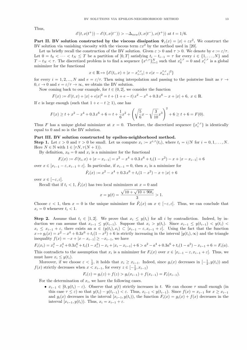
When t ≥ 1, this solution violates the local minimality.(iv) The BV solution constructed by epsilon-neighborhood method is

x(t) = 0 if t < 1 and x(t) =

√10 +

√10 + 90t

3if t > 1.

This solution coincides to the strong solution up to the strong solution exists. Moreover, it jumps att = 1 which is a physical relevant jump (see Fig. 2 and Fig. 3 below). The BV solution constructedby epsilon-neighborhood method satisfies the new energy-dissipation balance but it does not satisfythe energy-dissipation balance.

(v) The solution constructed by the method in [7] coincides to the solution in (iv).

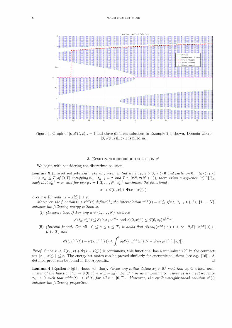
Notice that both solutions in (iii) and (iv) satisfy the definition of BV solutions [19, 20, 21]. Weak localstability in this case is: |∂xE (t, x(t))|∗ ≤ 1.

BV SOLUTIONS VIA EPSILON-NEIGHBORHOOD METHOD 5

−2 −1.5 −1 −0.5 0 0.5 1 1.5 26

8

10

12

14

16

18

x

E(t

,x)

+|x

|

Figure 1. E (t, x) + |x| with t = 1/6 in Example 2.

−2 −1.5 −1 −0.5 0 0.5 1 1.5 25

6

7

8

9

10

11

12

13

14

15

x

E(t

,x)

+|x

|

Figure 2. E (t, x) + |x| with t = 1 in Example 2.

6 MACH NGUYET MINH

t

x

abs(2 t x − 2 x + 4 x3 − (9 x

5)/5 + 1) − 1

0 0.2 0.4 0.6 0.8 1 1.2 1.4 1.6 1.8 2−2

−1.5

−1

−0.5

0

0.5

1

1.5

2

|∇ E(t,x)|=1

Domain where |∇ E(t,x)|>1

Solution in Case ii)

Solution in Case iii)

Solution in case iv)

Figure 3. Graph of |∂xE (t, x)|∗ = 1 and three different solutions in Example 2 is shown. Domain where|∂xE (t, x)|∗ > 1 is filled in.

3. Epsilon-neighborhood solution xε

We begin with considering the discretized solution.

Lemma 3 (Discretized solution). For any given initial state x0, ε > 0, τ > 0 and partition 0 = t0 < t1 <· · · < tN ≤ T of [0, T ] satisfying tn − tn−1 = τ and T ∈ [τN, τ(N + 1)), there exists a sequence {xε,τi }Ni=0

such that xε,τ0 = x0 and for every i = 1, 2, . . . , N , xε,τi minimizes the functional

x 7→ E (ti, x) + Ψ(x− xε,τi−1)

over x ∈ Rd with ‖x− xε,τi−1‖ ≤ ε.Moreover, the function t 7→ xε,τ (t) defined by the interpolation xε,τ (t) = xε,τi−1 if t ∈ [ti−1, ti), i ∈ {1, ..., N}

satisfies the following energy estimates.

(i) (Discrete bound) For any n ∈ {1, . . . , N} we have

E (tn, xε,τn ) ≤ E (0, x0) eλtn and E (0, xε,τn ) ≤ E (0, x0) e2λtn ;

(ii) (Integral bound) For all 0 ≤ s ≤ t ≤ T , it holds that DissΨ(xε,τ ; [s, t]) < ∞, ∂tE (·, xε,τ (·)) ∈L1(0, T ) and

E (t, xε,τ (t))− E (s, xε,τ (s)) ≤∫ t

s

∂tE (r, xε,τ (r)) dr −DissΨ(xε,τ ; [s, t]).

Proof. Since x 7→ E (tn, x) + Ψ(x− xε,τi−1) is continuous, this functional has a minimizer xε,τi in the compactset ‖x − xε,τi−1‖ ≤ ε. The energy estimates can be proved similarly for energetic solutions (see e.g. [16]). Adetailed proof can be found in the Appendix. �

Lemma 4 (Epsilon-neighborhood solution). Given any initial datum x0 ∈ Rd such that x0 is a local min-imizer of the functional x 7→ E (0, x) + Ψ(x − x0). Let xε,τ be as in Lemma 3. There exists a subsequenceτn → 0 such that xε,τn(t) → xε(t) for all t ∈ [0, T ]. Moreover, the epsilon-neighborhood solution xε(·)satisfies the following properties:

BV SOLUTIONS VIA EPSILON-NEIGHBORHOOD METHOD 7

(i) (Epsilon local stability) If xε(·) is right-continuous at t, namely limt′→t+ xε(t′) = xε(t), then xε(t)

satisfies the epsilon local stability

E (t, xε(t)) ≤ E (t, x) + Ψ(x− xε(t)) for all ‖x− xε(t)‖ ≤ ε;(ii) (Energy-dissipation inequalities) We have DissΨ(xε; [0, T ]) ≤ C (independent of ε), ∂tE (·, xε(·)) ∈

L1(0, T ) and for all 0 ≤ s ≤ t ≤ T ,

−Dissnew(xε; [s, t]) ≤ E (t, xε(t))− E (s, xε(s))−∫ t

s

∂tE (r, xε(r)) dr ≤ −DissΨ(xε; [s, t]).

Proof. Step 1. Existence. By the Integral bound in Lemma 3, the fact that E is non-negative, andcondition (7), we have

DissΨ(xε,τ ; [0, T ]) ≤ E (0, x0)− E (T, xε,τ (T )) +

∫ T

0

∂tE (r, xε,τ (r)) dr

≤ E (0, x0) +

N+1∑i=1

∫ ti

ti−1

λE (ti−1, xε,τi−1) eλ(r−ti−1) dr.

Here we denote T by tN+1. Using the Discrete bound in Lemma 3, we get

DissΨ(xε,τ ; [0, T ]) ≤ E (0, x0) +

∫ T

0

λE (0, x0) eλr dr = E (0, x0) eλT .

Thus, {xε,τ (·)} has uniformly bounded variation and it is uniformly bounded. Therefore, applying Helly’sselection principle [12, 1, 27], we can find a subsequence τn → 0 and a BV function xε(·) such thatxε,τn(t)→ xε(t) as n→∞ for all t ∈ [0, T ].

Step 2. A consequence of the right-continuity. Let us denote by {tni }Nni=0 the partition corresponding

to τn and assume that t ∈ [tni−1, tni ). It is obvious that

xε,τni−1 = xε,τn(t)→ xε(t)

as n→∞. Now we show that if xε(·) is right-continuous at t, then

xε,τni = xε,τn(tni )→ xε(t).

Let t′ > t. Thanks to the Integral bound in Lemma 3, we have

E (t′, xε,τn(t′))− E (t, xε,τn(t)) + DissΨ(xε,τn ; [t, t′]) ≤∫ t′

t

∂tE (r, xε,τn(r)) dr ≤ C|t′ − t|.

Here the last inequality is due to the continuity of ∂tE and the fact that xε,τn is bounded on [0, T ]. For nlarge enough, we have t < tni < t′. Therefore,

Ψ(xε,τni − xε,τni−1 ) ≤ DissΨ(xε,τn ; [t, t′]).

Moreover, when n→∞, we get

xε,τn(t)→ xε(t) and xε,τn(t′)→ xε(t′).

Thus it follows from the above integral bound that

E (t′, xε(t′))− E (t, xε(t)) + lim supn→∞

Ψ(xε,τni − xε,τni−1 ) ≤ C|t′ − t|.

Notice that the inequality above holds for all t′ > t. Hence, we can take t′ → t and use the assumptionxε(t+) = xε(t) to obtain

lim supn→∞

Ψ(xε,τni − xε,τni−1 ) ≤ 0.

Since xε,τni−1 → xε(t), we can conclude that xε,τni → xε(t) as n→∞.

Step 3. Stability. We show that for all t ∈ [0, T ], if xε(·) is right-continuous at t, then

E (t, xε(t)) ≤ E (t, z) + Ψ(z − xε(t)) for all ‖z − xε(t)‖ ≤ ε.To this end, we first prove the result for z ∈ Rd with ‖z − xε(t)‖ < ε. Since limn→∞ xε,τn(t) = xε(t), we

get‖z − xε,τn(t)‖ < ε

8 MACH NGUYET MINH

for n large enough. We shall follow the notations in Step 2. The fact that t ∈ [tni−1, tni ) yields xε,τn(t) = xε,τni−1 .

From the definition of xε,τni and condition ‖z − xε,τni−1 ‖ < ε, we obtain

E (tni , xε,τni ) + Ψ(xε,τni − xε,τni−1 ) ≤ E (tni , z) + Ψ(z − xε,τni−1 ).

Taking the limit as n → ∞ and using the fact that both xε,τni−1 and xε,τni converge to xε(t) (see Step 2), wehave

E (t, xε(t)) ≤ E (t, z) + Ψ(z − xε(t)) for all ‖z − xε(t)‖ < ε.(9)

Now for any z satisfying ‖z − xε(t)‖ = ε, we can choose a sequence zn converging to z such that ‖zn −xε(t)‖ < ε. Applying (9) for zn, we get

E (t, xε(t)) ≤ E (t, zn) + Ψ(zn − xε(t)).(10)

Note that the mapping y 7→ E (t, y)+Ψ(y−xε(t)) is continuous, taking the limit in (10), we obtain the resultalso for ‖z − xε(t)‖ = ε.

Step 4. Energy-dissipation inequalities.By the Integral bound in Lemma 3, we have for all 0 ≤ s ≤ t ≤ T ,

E (t, xε,τn(t))− E (s, xε,τn(s)) ≤∫ t

s

∂tE (r, xε,τn(r)) dr −DissΨ(xε,τn ; [s, t]).

Since xε,τn(r)→ xε(r) for all r ∈ [0, T ], we have

E (t, xε,τn(t))− E (s, xε,τn(s))→ E (t, xε(t))− E (s, xε(s))

and ∫ t

s

∂tE (r, xε,τn(r)) dr →∫ t

s

∂tE (r, xε(r)) dr

as n→∞. Moreover, one has

lim infn→∞

DissΨ(xε,τn ; [s, t]) ≥ DissΨ(xε; [s, t]).

Thus we can derive one energy-dissipation inequality

E (t, xε(t))− E (s, xε(s)) ≤∫ t

s

∂tE (r, xε(r)) dr −DissΨ(xε; [s, t]).

We shall use Lemma 5 to obtain the other energy-dissipation inequality,

E (t, xε(t))− E (s, xε(s)) ≥∫ t

s

∂tE (r, xε(r)) dr −Dissnew(xε; [s, t]).(11)

To apply Lemma 5, it is sufficient to verify that −∇xE (t, xε(t)) ∈ ∂Ψ(0) for a.e. t ∈ (0, T ). Indeed, for everyt ∈ [0, T ] such that xε(·) is right-continuous at t, we have proved in Step 3 the ε-stability

E (t, xε(t)) ≤ E (t, x) + Ψ(x− xε(t)) for all ‖x− xε(t)‖ ≤ ε.

For every x satisfying ‖x − xε(t)‖ ≤ ε and for every s ∈ [0, 1], denote by z = xε(t) + s(x − xε(t)). Clearly,‖z − xε(t)‖ ≤ ε. Thus,

E (t, xε(t)) ≤ E (t, z) + Ψ(z − xε(t)).This inequality is equivalent to

E (t, xε(t))− E (t, xε(t) + s(x− xε(t)))s

≤ Ψ(x− xε(t)).

Taking s→ 0+ and notice that E is of class C1, we obtain that

〈−∇xE (t, xε(t)), x− xε(t)〉 ≤ Ψ(x− xε(t)) for all ‖x− xε(t)‖ ≤ ε.

Now for every y ∈ Rd\{0}, applying the inequality above for y = xε(t) + εy/‖y‖, we get

〈−∇xE (t, xε(t)), y〉 ≤ Ψ(y).

Hence, −∇xE (t, xε(t)) ∈ ∂Ψ(0) whenever xε(t) is right-continuous at t.On the other hand, since xε(·) is a BV function, it is continuous except at most countably many points.

Thus, we can conclude that −∇xE (t, xε(t)) ∈ ∂Ψ(0) for a.e. t ∈ (0, T ). �

BV SOLUTIONS VIA EPSILON-NEIGHBORHOOD METHOD 9

Lemma 5 (Lower bound of the new energy-dissipation balance). For any BV function u : [0, T ] → Rd,energy functional E ∈ C1([0, T ] × Rd) and dissipation functional Ψ which is convex and positively 1-homogeneous, if −∇xE (t, u(t)) ∈ ∂Ψ(0) for a.e. t ∈ (0, T ), it holds that

E (t1, u(t1))− E (t0, u(t0)) ≥∫ t1

t0

∂tE (s, u(s)) ds−Dissnew(u; [t0, t1]), for all 0 ≤ t0 < t1 ≤ T.

This result is due to Mielke, Rossi and Savare (see [20, Proposition 4.2] for finite-dimensional space and[21, Theorem 3.11] for infinite-dimensional space). For the readers’ convenience, a proof of Lemma 5 isincluded in Appendix.

4. BV solutions constructed by epsilon-neighborhood method

Lemma 6 (Limit of epsilon-neighborhood solutions). Given an initial datum x0 ∈ Rd which is a localminimizer of the functional x 7→ E (0, x) + Ψ(x− x0). Let xε be as in Lemma 4. There exists a subsequenceεn → 0 and a BV function u such that xεn(t)→ u(t) for all t ∈ [0, T ]. Moreover, the function u satisfies thefollowing properties

(i) (Weak local stability) If t 7→ u(t) is continuous at t, then

−∇xE (t, u(t)) ∈ ∂Ψ(0);

(ii) (New energy-dissipation balance) For all 0 ≤ s ≤ t ≤ T , one has

E (t, u(t))− E (s, u(s)) =

∫ t

s

∂tE (r, u(r)) dr −Dissnew(u; [s, t]).

Proof. Step 1. Existence. Since DissΨ(xε; [0, T ]) ≤ C independent of ε, by Helly’s selection principle wecan find a subsequence εn → 0 and a BV function u such that xεn(t)→ u(t) as n→∞ for all t ∈ [0, T ].

Step 2. Stability. Let

A := {t ∈ [0, T ] |xεn(·) is right continuous at t for all n ≥ 1}.

Then [0, T ]\A is at most countable. Moreover, for t ∈ A, by Lemma 4 we get

E (t, xεn(t)) ≤ E (t, z) + Ψ(z − xεn(t)) for all ‖z − xεn(t)‖ ≤ εnfor all n ≥ 1. For t ∈ A and n ≥ 1,

〈−∇xE (t, xεn(t)), z〉 ≤ Ψ(z) for all z ∈ Rd

can be shown in a similar manner as in Step 4, Lemma 4. Taking n→∞, we obtain

〈−∇xE (t, u(t)), z〉 ≤ Ψ(z) for all z ∈ Rd, for all t ∈ A.

By continuity, we immediately have −∇xE (t, u(t)) ∈ ∂Ψ(0) provided that u is continuous at t.

Step 3. New energy-dissipation balance. By means of a similar proof of the energy inequalitiesin Lemma 4, we have

−Dissnew(u; [s, t]) ≤ E (t, u(t))− E (s, u(s))−∫ t

s

∂tE (r, u(r)) dr ≤ −Diss(u; [s, t]).

(The second inequality is a consequence of the corresponding inequality of xε in Lemma 4 and Fatou’s lemma,while the first inequality follows from Lemma 5.)

Notice that if the solution t 7→ u(t) is continuous on [a, b] ⊂ [0, T ], then Diss(u; [a, b]) = Dissnew(u; [a, b]).Thus, we have immediately the energy-dissipation balance

E (b, u(b))− E (a, u(a))−∫ b

a

∂tE (r, u(r)) dr = −Diss(u; [a, b]) = −Dissnew(u; [a, b]).

Therefore, it remains to consider jump points. More precisely, we need to show that if u jumps att ∈ (0, T ), namely u(t−) 6= u(t+), then

E (t, u(t+))− E (t, u(t−)) = −∆new(t, u(t−), u(t))−∆new(t, u(t), u(t+)).

This fact follows from Lemma 5, 7 and 8. �

10 MACH NGUYET MINH

To prove the upper bound, we start by showing that the discretized solution xε,τ is “almost” an optimaltransition.

Lemma 7 (Approximate optimal transition). For the discretized solution xε,τ , if we write xj := xε,τ (tj), itholds that

〈−∇xE (ti, xi), xi − xi−1〉 = Ψ(xi − xi−1) + minη∈∂Ψ(0)

‖η +∇xE (ti, xi)‖∗ · ‖xi − xi−1‖.

Consequently, if δ ≥ ε+ |t− ti| and v : [a, b]→ Rd is the linear curve connecting xi−1 and xi, namely

v(s) = xi−1 +s− ab− a

(xi − xi−1),

there exists g(δ) such that g(δ)→ 0 as δ → 0 and

E (t, xi−1)− E (t, xi) ≥∫ b

a

Ψ(v(s)) + minη∈∂Ψ(0)

‖η +∇xE (t, v(s))‖∗ · ‖v(s)‖ ds− (b− a)g(δ)‖xi − xi−1‖.

Proof. The proof is trivial when xi = xi−1. Hence, we shall assume that xi 6= xi−1.

Step 1. Denote by m(z) := ‖z− xi−1‖ and h(z) := E (ti, z) + Ψ(z− xi−1). Recall that xi is a minimizer for

infm(z)≤ε

h(z).

Denote by c := ‖xi − xi−1‖. Since c ≤ ε, we can consider xi as a minimizer for

infm(z)=c

h(z).

Here (xi − xi−1)T stands for the transpose of (xi − xi−1). By Lagrange multiplier, there exists λ ∈ R suchthat λ∇m(xi) ∈ ∂h(xi), or equivalently

λ(xi − xi−1)T

‖xi − xi−1‖− ∇xE (ti, xi) ∈ ∂Ψ(xi − xi−1).

The inclusion above implies two following conditions

i. For all z ∈ Rd, it holds that⟨−∇xE (ti, xi) + λ (xi−xi−1)T

‖xi−xi−1‖ , z⟩≤ Ψ(z).

ii.⟨−∇xE (ti, xi) + λ (xi−xi−1)T

‖xi−xi−1‖ , xi − xi−1

⟩= Ψ(xi − xi−1).

Step 2. Since the function h1(s) = h(xi−1 + s(xi − xi−1)) satisfies h1(s) ≥ h1(1) for all s ∈ [0, 1], it followsthat

E (ti, xi−1 + s(xi − xi−1)) + sΨ(xi − xi−1) ≥ E (ti, xi) + Ψ(xi − xi−1).

The above inequality can be rewritten as

E (ti, xi + (s− 1)(xi − xi−1))− E (ti, xi)

s− 1+ Ψ(xi − xi−1) ≤ 0.

Since E is of class C1, we can conclude that

〈∇xE (ti, xi), xi − xi−1〉+ Ψ(xi − xi−1) ≤ 0.(12)

In addition, (12) and Condition ii) in Step 1 give λ ≤ 0. Moreover, for all η ∈ ∂Ψ(0) we have −Ψ(xi−xi−1) ≤〈−η, xi − xi−1〉. Thus, condition ii) implies

−λ⟨(xi − xi−1)T , xi − xi−1

⟩‖xi − xi−1‖

= 〈−∇xE (ti, xi), xi − xi−1〉 −Ψ(xi − xi−1)

≤ 〈−∇xE (ti, xi)− η, xi − xi−1〉≤ ‖ −∇xE (ti, xi)− η‖∗ · ‖xi − xi−1‖.

Thanks to Condition i) in Step 1, η0 ∈ ∂Ψ(0), where η0 is chosen so that η0 = −∇xE (ti, xi)− k(xi− xi−1)T

and k = − λ‖xi−xi−1‖ ≥ 0. Moreover, the above two inequalities becomes equalities with such choice of η0.

Thus, we can write

−λ⟨(xi − xi−1)T , xi − xi−1

⟩‖xi − xi−1‖

= minη∈∂Ψ(0)

‖η +∇xE (ti, xi)‖∗ · ‖xi − xi−1‖.

BV SOLUTIONS VIA EPSILON-NEIGHBORHOOD METHOD 11

Hence, we obtain that

〈−∇xE (ti, xi), xi − xi−1〉 = Ψ(xi − xi−1) + minη∈∂Ψ(0)

‖η +∇xE (ti, xi)‖∗ · ‖xi − xi−1‖.

Step 3. Consequently, using |t − ti| ≤ δ, ‖xi−1 − xi‖ ≤ ε ≤ δ and the fact that ∇xE (·, ·) is continuous oncompact sets, there exists g(δ) such that g(δ)→ 0 when δ → 0 and

〈−∇xE (t, v(s)), v(s)〉 ≥ Ψ(v(s)) + minη∈∂Ψ(0)

‖η +∇xE (t, v(s))‖∗ · ‖v(s)‖ − g(δ) ‖v(s)‖

for every s ∈ [a, b]. Therefore,

E (t, xi−1)− E (t, xi) =

∫ b

a

〈−∇xE (t, v(s)), v(s)〉 ds

≥∫ b

a

Ψ(v(s)) + minη∈∂Ψ(0)

‖η +∇xE (t, v(s))‖∗ · ‖v(s)‖ ds− (b− a)g(δ)‖xi − xi−1‖.

�

Now we are in the position to prove the new energy-dissipation upper bound at jumps.

Lemma 8 (Upper bound). Let u be the function as in Lemma 6. If u(t−) 6= u(t), then

∆new(t, u(t−), u(t)) ≤ E (t, u(t−))− E (t, u(t)).

Proof. Let 0 � τ � ε � δ � 1. By the definition of the discretized solution xε,τ , for every t ∈ (0, T ) wehave

xε,τ (t− δ) = xε,τ (ti) and xε,τ (t) = xε,τ (ti+k)

for ti, ti+k ∈ [t− 2δ, t+ δ].We can construct an absolutely continuous function v : [0, 1]→ Rd by linearly interpolating the following

(k + 3) points:

u(t−), xε,τ (t− δ) = xε,τ (ti), xε,τ (ti+1), . . . , xε,τ (ti+k) = xε,τ (t), u(t).

More precisely, we definez0 = u(t−),

z1 = xε,τ (t− δ) = xε,τ (ti),

z2 = xε,τ (ti+1),

. . .

zk+1 = xε,τ (ti+k) = xε,τ (t),

zk+2 = u(t),

and denote r := 1/(k + 2) and

v(s) = zj +s− jrr

(zj+1 − zj) when s ∈ [jr, (j + 1)r], j = 0, 1, . . . , k + 1.

By the definition of the new dissipation, we have

∆new(t, u(t−), u(t)) ≤∫ 1

0

Ψ(v(s)) + minη∈∂Ψ(0)

‖η +∇xE (t, v(s))‖∗ · ‖v(s)‖ ds

=

k+1∑j=0

∫ (j+1)r

jr

Ψ(v(s)) + minη∈∂Ψ(0)

‖η +∇xE (t, v(s))‖∗ · ‖v(s)‖ ds.

When j = 0 and j = k + 1, we estimate∫ (j+1)r

jr

Ψ(v(s)) + minη∈∂Ψ(0)

‖η +∇xE (t, v(s))‖∗ · ‖v(s)‖ ≤ C∫ (j+1)r

jr

‖v(s)‖ ds = C‖zj+1 − zj‖.

When j = 1, 2, . . . , k, Lemma 7 yields the following equation∫ (j+1)r

jr

Ψ(v(s)) + minη∈∂Ψ(0)

‖η +∇xE (t, v(s))‖∗ · ‖v(s)‖ ds ≤ E (t, xε,τ (ti+j−1))− E (t, xε,τ (ti+j))

+rg(δ) · ‖xε,τ (ti+j)− xε,τ (ti+j−1)‖,

12 MACH NGUYET MINH

where g(δ)→ 0 as δ → 0. Taking the sum over j = 0, 1, . . . , k+1 and using the bound DissΨ(xε,τ ; [0, T ]) ≤ C(independent of ε and τ), we find that

∆new(t, u(t−), u(t)) ≤∫ 1

0

Ψ(v(s)) + minη∈∂Ψ(0)

‖η +∇xE (t, v(s))‖∗ · ‖v(s)‖ ds

≤ E (t, xε,τ (t− δ))− E (t, xε,τ (t)) + Cg(δ) + C‖u(t−)− xε,τ (t− δ)‖+ C‖xε,τ (t)− u(t)‖.Taking the limit τ → 0, then ε→ 0, then δ → 0, we conclude that

∆new(t, u(t−), u(t)) ≤ E (t, u(t−))− E (t, u(t)).

This finishes the proof. �

5. Appendix: Technical proofs

5.1. Example 2. First of all, it is easy to verify that E (t, x) : [0, 2] × R → [0,+∞) is C1 and satisfiescondition (6). Moreover, x0 = 0 is a local minimizer for the functional x 7→ E (0, x) + |x|.

Part I. Energetic solution via time-discretization.Step 1. Fix a time step τ > 0. To find the discretized solution xτ (t), it suffices to calculate xi := xτ (ti)where 0 = t0 < · · · < tN ≤ 1 and ti− ti−1 = τ for all i = 1, 2, . . . , N. Here N ∈ N satisfies 1 ∈ [τN, τ(N+1)).

We have x0 = 0 and for all i = 1, 2, . . . , N , xi is a minimizer of the functional

x ∈ R 7→ E (ti, x) + |x− xi−1|.Step 2. Let us fix t ∈ (0, 2] and consider the functional

F (x) := E (t, x) + |x| = x2 − x4 + 0.3x6 + t(1− x2)− x+ |x|+ 6, x ∈ R.It is readily seen that

• When t ≤ 1, F (x) has two local minimizers (see Fig. 1)

x = 0 and x = y(t) :=

√10 +

√10 + 90t

3.

Moreover,

F (y(t))− F (0) =1

243(10 +

√10 + 90t)(8− 18t−

√10 + 90t),

which is positive if t < 1/6 and negative if t > 1/6. Hence F has a unique global minimizer x = 0 if0 ≤ t < 1/6, and then F has a unique global minimizer at x = y(t) if 1/6 < t < 1.• When t > 1, F (x) has a unique local (also global) minimizer at x = y(t).

Step 3. By induction, we can show that if ti0 < 1/6 ≤ ti0+1, then xi = 0 for all i = 1, 2, ..., i0, and eitherxi0+1 = y(ti0+1), or xi0+1 = 0 and xi0+2 = y(ti0+2).

Next, we show that if ti−1 ≥ 1/6 and xi−1 = y(ti−1) > 0, then xi = y(ti). Recall that xi is a globalminimizer for the functional

x ∈ R 7→ Fi(x) := E (ti, x) + |x− xi−1| = x2 − x4 + 0.3x6 + ti(1− x2)− x+ |x− xi−1|+ 6.

By using the triangle inequality −x+ |x− xi−1| ≥ −xi−1 and the same analysis of F , we can conclude thatxi = y(ti).

Taking the limit as τ → 0, we obtain the energetic solution

x(t) = 0 if t ∈ [0, 1/6), x(1/6) ∈ {0,√

5/3}, x(t) = y(t) if t ∈ [1/6, 2].

Step 4. Finally, we show that the energetic solution does not satisfies the new energy-dissipation balance.It suffices to show that at the jump point t = 1/6,

E (t, x(t+))− E (t, x(t−)) > −∆new(t, x(t−), x(t+)).

Indeed, a direct computation gives us that at t = 1/6,

E (t, x(t+))− E (t, x(t−)) = E (1/6,√

5/3)− E (1/6, 0) = −√

5/3.

On the other hand, at t = 1/6 we have

∆new(t, x(t−), x(t+)) =

∫ √15/3

0

max

{1,

∣∣∣∣23y − 4y3 + 1.8y5 − 1

∣∣∣∣} dy =185

486+

√5

3.

BV SOLUTIONS VIA EPSILON-NEIGHBORHOOD METHOD 13

Thus,E (t, x(t+))− E (t, x(t−)) > −∆new(t, x(t−), x(t+)) at t = 1/6.

Part II. BV solution constructed by the viscous dissipation Ψε(x) = |x| + εx2. We construct theBV solution via vanishing viscosity with the viscous term εx2 by the method used in [20].

Let us briefly recall the construction of the BV solution. Given ε > 0 and τ > 0. We denote by e := ε/τ .Let 0 = t0 < · · · < tN ≤ T be a partition of [0, T ] satisfying ti − ti−1 = τ for every i ∈ {1, . . . , N} andT − tN < τ . The discretized problem is to find a sequence {xε,τ}Ni=1 such that xε,τ0 = 0 and xε,τi is a globalminimizer for the functional

x ∈ R 7→ {E (ti, x) + |x− xτ,εi−1|+ e|x− xτ,εn−1|2}for every i = 1, 2, ..., N and e = ε/τ. Then using interpolation and passing to the pointwise limit as τ →0, ε→ 0 and e = ε/τ →∞, we obtain the BV solution.

Now coming back to our example, for t ∈ (0, 2], we consider the function

F (x) := E (t, x) + |x|+ e|x|2 = t+ (1 + e− t)x2 − x4 + 0.3x6 − x+ |x|+ 6, x ∈ R.If e is large enough (such that 1 + e− t ≥ 1), one has

F (x) ≥ t+ x2 − x4 + 0.3x6 + 6 = t+1

6x2 +

(√5

6x−

√3

10x3

)2

+ 6 ≥ t+ 6 = F (0).

Thus F has a unique global minimizer at x = 0. Therefore, the discretized sequence {xτ,εi } is identicallyequal to 0 and so is the BV solution.

Part III. BV solution constructed by epsilon-neighborhood method.Step 1. Let ε > 0 and τ > 0 be small. Let us compute xi := xε,τ (ti), where ti = i/N for i = 0, 1, . . . , N .Here N ∈ N with 1 ∈ [τN, τ(N + 1)).

By definition, x0 = 0 and xi is a minimizer for the functional

Fi(x) := E (ti, x) + |x− xi−1| = x2 − x4 + 0.3x6 + ti(1− x2)− x+ |x− xi−1|+ 6

over x ∈ [xi−1 − ε, xi−1 + ε]. In particular, if xi−1 = 0, then xi is a minimizer for

Fi(x) := x2 − x4 + 0.3x6 + ti(1− x2)− x+ |x|+ 6

over x ∈ [−ε, ε].Recall that if ti < 1, Fi(x) has two local minimizers at x = 0 and

x = y(t) =

√10 +

√10 + 90ti

3> 1.

Choose ε < 1, then x = 0 is the unique minimizer for Fi(x) on x ∈ [−ε, ε]. Thus, we can conclude thatxi = 0 whenever ti < 1.

Step 2. Assume that ti ∈ [1, 2]. We prove that xi ≤ y(ti) for all i by contradiction. Indeed, by in-duction we can assume that xi−1 ≤ y(ti−1). Suppose that xi > y(ti). Since xi−1 ≤ y(ti−1) < y(ti) <xi ≤ xi−1 + ε, there exists an a ∈ (y(ti), xi) ⊂ [xi−1 − ε, xi−1 + ε]. Using the fact that the functionx 7→ gi(x) = x2 − x4 + 0.3x6 + ti(1− x2) + 6 is strictly increasing in the interval [y(ti),∞) and the triangleinequality f(x) = −x+ |x− xi−1| ≥ −xi−1, we have

Fi(xi) = x2i − x4

i + 0.3x6i + ti(1− x2

i )− xi + |xi − xi−1|+ 6 > a2 − a4 + 0.3a6 + ti(1− a2)− xi−1 + 6 = Fi(a).

This contradicts to the assumption that xi is a minimizer for Fi(x) over x ∈ [xi−1 − ε, xi−1 + ε]. Thus, wemust have xi ≤ y(ti).

Moreover, if we choose ε < 12 , it holds that xi ≥ xi−1. Indeed, since gi(x) decreases in [− 1

2 , y(ti)) and

f(x) strictly decreases when x < xi−1, for every z ∈ [− 12 , xi−1)

Fi(z) = gi(z) + f(z) > gi(xi−1) + f(xi−1) = Fi(xi−1).

For the determination of xi, we have the following cases.

• xi−1 ∈ [0, y(ti) − ε). Observe that y(t) strictly increases in t. We can choose τ small enough (inthis case τ ≤ ε) so that y(ti) − y(ti−1) < ε. Thus, xi−1 < y(ti−1). Since f(x) = xi−1 for x ≥ xi−1

and gi(x) decreases in the interval [xi−1, y(ti)), the function Fi(x) = gi(x) + f(x) decreases in theinterval [xi−1, y(ti)). Thus, xi = xi−1 + ε.

14 MACH NGUYET MINH

• For the case when xi−1 ∈ [y(ti) − ε, y(ti−1)], y(ti) is the unique minimizer of Fi(x) in the interval[xi−1, xi−1 + ε]. Thus, xi = y(ti).

Step 3. Taking the largest k and the smallest m such that xk = 0 and xm = y(tm). The number of steps L

to move from xk to xm is the integer part of y(tm)ε . Since ε is fixed, this value is bounded from above by a

constant C =[

5ε

]+ 1. Hence,

tm = tk + Lτ ≤ tk + Cτ.

Taking τ → 0, we have tm ≈ tk ≈ 1. Thus, for ε < 12 , the BV solution constructed by epsilon-neighborhood

method is x(t) = xε(t) = 0 if t ∈ [0, 1) and x(t) = xε(t) = y(t) if t ∈ (1, 2]. At t = 1, x(t) can take valueseither 0 or y(1).

Step 4. We show that the BV solution constructed by epsilon-neighborhood does not satisfy the energy-dissipation balance. At the jump point t = 1, one has

−|x(t−)− x(t+)| = −2√

5

3> E (t, x(t+))− E (t, x(t−)) = −400

243−√

20

3.

Part IV. The solution constructed by the method in [7]. Let us briefly recall the method used in[7]. Let N ∈ N be the numbers of time step. The neighborhood is chosen equal to the usual time-step, i.e.ε = τ = T

N . Take t0 = 0 and x0 = 0. For j = 1, . . . , N , xj and tj are defined as follows.

• xj minimizes {E (tj−1, x) + |x− xj−1|} among all states x such that |x− xj−1| ≤ ε.• tj = tj−1 + τ − |xj − xj−1|.

By the same argument as in Part III, Step 1, we deduce that xi+1 = 0 and ti+1 = ti+ τ if N < T and ti < 1.Now assume that ti ∈ [1, 2]. Argue as in Part III, Step 2, we have xi+1 ∈ [xi, y(ti)] and

• If xi ∈ [0, y(ti)− ε): xi+1 = xi + ε and ti+1 = ti.• If xi ∈ [y(ti)− ε, y(ti−1)]: xi+1 = y(ti) and ti+1 = ti + τ − |y(ti)− xi|.

Taking τ to 0, we obtain the solution x(t) = 0 if t < 1, x(t) = y(t) if t ≥ 1.

5.2. Proof of the energy estimate in Lemma 3. Step 1. By the minimality of xε,τn at time tn, we have

E (tn, xε,τn ) + Ψ(xε,τn − x

ε,τn−1) ≤ E (tn, x

ε,τn−1) = E (tn−1, x

ε,τn−1) +

∫ tn

tn−1

∂tE (t, xε,τn−1) dt.

It follows from the assumption (7) that

∂tE (t, xε,τn−1) ≤ λE (tn−1, xε,τn−1) eλ(t−tn−1) for all t ∈ [tn−1, tn].

Applying Gronwall’s inequality we obtain

E (tn, xε,τn ) ≤ E (tn, x

ε,τn ) + Ψ(xε,τn − x

ε,τn−1)

≤∫ tn

tn−1

λE (tn−1, xε,τn−1) eλ(t−tn−1)dt+ E (tn−1, x

ε,τn−1)

= E (tn−1, xε,τn−1)(eλ(tn−tn−1) − 1) + E (tn−1, x

ε,τn−1) = E (tn−1, x

ε,τn−1) eλ(tn−tn−1).

By induction,

E (tn, xε,τn ) ≤ E (tn−1, x

ε,τn−1) eλ(tn−tn−1) ≤ E (tn−2, x

ε,τn−2) eλ(tn−1−tn−2) eλ(tn−tn−1)

≤ · · · ≤ E (0, x0) eλ(t1−t0) eλ(t2−t1) . . . eλ(tn−tn−1) = E (0, x0) eλtn .

Finally, by (7) again,

E (0, xε,τn ) ≤ E (tn, xε,τn ) eλtn ≤ E (0, x0) e2λtn .

Step 2. Now we prove the integral bound. Assume that ti−1 < s ≤ ti < ti+1 < · · · < tj ≤ t < tj+1, where{tn} is the partition corresponding to xε,τ . We start by writing

E (t, xε,τ (t))− E (s, xε,τ (s)) = E (t, xε,τ (t))− E (tj , xε,τ (tj)) + . . .(13)

+E (tj , xε,τ (tj))− E (tj−1, x

ε,τ (tj−1)) + E (ti, xε,τ (ti))− E (s, xε,τ (s)).

BV SOLUTIONS VIA EPSILON-NEIGHBORHOOD METHOD 15

By the minimality of xk := xε,τ (tk) at time tk, we have

E (tk, xk)− E (tk−1, xk−1) ≤ E (tk, xk−1)−Ψ(xk − xk−1)− E (tk−1, xk−1) =

∫ tk

tk−1

∂tE (r, xk−1) dr −Ψ(xk − xk−1).

Taking the sum for all k from i+ 1 to j and using xε,τ (r) = xk−1 for all r ∈ [tk−1, tk), we get

j∑k=i+1

[E (tk, xk)− E (tk−1, xk−1)] ≤j∑

k=i+1

∫ tk

tk−1

∂tE (r, xε,τ (r)) dr −j∑

k=i+1

Ψ(xk − xk−1).(14)

Moreover, since ti−1 < s ≤ ti and tj ≤ t < tj+1, we can write

E (ti, xε,τ (ti))− E (s, xε,τ (s)) = E (ti, xi)− E (s, xi−1)

≤ E (ti, xi−1)−Ψ(xi − xi−1)− E (s, xi−1)

=

∫ ti

s

∂tE (r, xε,τ (r)) dr −Ψ(xi − xε,τ (s)).(15)

E (t, xε,τ (t))− E (tj , xε,τ (tj)) = E (t, xj)− E (tj , xj) =

∫ t

tj

∂tE (r, xε,τ (r)) dr −Ψ(xε,τ (t)− xj),(16)

Thus, it follows from (13), (14), (16) and (15) that

E (t, xε,τ (t))− E (s, xε,τ (s)) ≤∫ t

s

∂tE (r, xε,τ (r)) dr −

(Ψ(xε,τ (t)− xj) +

j∑k=i+1

Ψ(xk − xk−1) + Ψ(xi − xε,τ (s))

)

=

∫ t

s

∂tE (r, xε,τ (r)) dr −DissΨ(xε,τ ; [s, t]).

5.3. Proof of Lemma 5.

Proof. Applying the chain rule formula for E ∈ C1 and u ∈ BV (see [2]), we get

E (t1, u(t1))− E (t0, u(t0)) =

∫ t1

t0

∂tE (s, u(s)) ds+

∫ t1

t0

〈∇xE (s, u(s)), u′co(s)〉 ds

+∑

t∈J∩(t0,t1)

[E (t, u(t))− E (t, u(t−))

]+

∑t∈J∩(t0,t1)

[E (t, u(t+))− E (t, u(t))

]+E (t0, u(t+0 ))− E (t0, u(t0)) + E (t1, u(t1))− E (t1, u(t−1 )).

The fact that −∇xE (t, u(t)) ∈ ∂Ψ(0) whenever u(t) is continuous at t yields∫ t1

t0

〈∇xE (s, u(s)), u′co(s)〉 ds ≥ −∫ t1

t0

Ψ(u′co(s)) ds.(17)

Notice that∫ t1

t0

Ψ(u′co(s)) ds = Diss(u; [t0, t1])−∑

t∈J∩(t0,t1)

Ψ(u(t)− u(t−))−∑

t∈J∩(t0,t1)

Ψ(u(t+)− u(t))

−Ψ(u(t+0 )− u(t0))−Ψ(u(t1)− u(t−1 )).(18)

Moreover, for every absolutely continuous curve v in AC([0, 1];Rd) such that v(0) = u(t−), v(1) = u(t) wehave

|E (t, u(t))− E (t, u(t−))| =

∣∣∣∣∫ 1

0

〈∇xE (t, v(s)), v(s)〉 ds∣∣∣∣ .

For any η ∈ ∂Ψ(0), it holds that 〈η, v〉 ≤ Ψ(v) for all v ∈ Rd. Thus, at every point s ∈ [0, 1] for which thederivative v(s) exists, we can write

−Ψ(v(s)) ≤ 〈−η, v(s)〉 .Hence,

〈−∇xE (t, v(s)), v(s)〉 = Ψ(v(s))−Ψ(v(s)) + 〈−∇xE (t, v(s)), v(s)〉≤ Ψ(v(s)) + 〈−η, v(s)〉+ 〈−∇xE (t, v(s)), v(s)〉≤ Ψ(v(s)) + ‖ − η −∇xE (t, v(s))‖∗ · ‖v(s)‖.

16 MACH NGUYET MINH

The inequality above holds for every η ∈ ∂Ψ(0). Thus, we obtain

〈−∇xE (t, v(s)), v(s)〉 ≤ Ψ(v(s)) + infη∈∂Ψ(0)

‖η +∇xE (t, v(s))‖∗ · ‖v(s)‖.

Therefore, for any absolutely continuous curve v in AC([0, 1];Rd) satisfying v(0) = u(t−), v(1) = u(t), itholds that

|E (t, u(t))− E (t, u(t−))| ≤∫ 1

0

Ψ(v(s)) + infη∈∂Ψ(0)

‖η +∇xE (t, v(s))‖∗ · ‖v(s)‖.

By the definition of ∆new(t, u(t−), u(t)), we can conclude that

|E (t, u(t))− E (t, u(t−))| ≤ ∆new(t, u(t−), u(t)).(19)

Similarly, we also get

|E (t, u(t+))− E (t, u(t))| ≤ ∆new(t, u(t), u(t+)).(20)

Thus, it follows from (17), (18), (19) and (20) that

E (t1, u(t1))− E (t0, u(t0)) ≥∫ t1

t0

∂tE (s, u(s)) ds−Diss(u; [t0, t1])

+∑

t∈J∈(t0,t1)

Ψ(u(t−)− u(t)) +∑

t∈J∈(t0,t1)

Ψ(u(t)− u(t+))

+Ψ(u(t0)− u(t+0 )) + Ψ(u(t−1 )− u(t1))

−∑

t∈J∩(t0,t1)

∆new(t, u(t−), u(t))−∑

t∈J∩(t0,t1)

∆new(t, u(t), u(t+))

−∆new(t0, u(t0), u(t+0 ))−∆new(t1, u(t−1 ), u(t1))

=

∫ t1

t0

∂tE (s, u(s)) ds−Dissnew(u; [t0, t1]).

This ends the proof of Lemma 5. �

References

[1] G. Alberti and A. DeSimone, Quasistatic evolution of sessile drops and contact angle hysteresis, Arch. Rational Mech.

Anal., 202 (2011), pp. 295–348.[2] L. Ambrosio, N. Fusco, and D. Pallara, Functions of bounded variation and free discontinuity problems, Clarendon

Press, 2000.[3] G. Dal Maso, A. DeSimone, M. G. Mora, and M. Morini, Globally stable quasistatic evolution in plasticity with

softening, Netw. Heterog. Media, 3 (2008), pp. 567–614.

[4] , A vanishing viscosity approach to quasistatic evolution in plasticity with softening, Arch. Ration. Mech. Anal., 189(2008), pp. 469–544.

[5] G. Dal Maso, A. DeSimone, and F. Solombrino, Quasistatic evolution for Cam-Clay plasticity: a weak formulationvia viscoplastic regularization and time rescaling, Cal. Var. and PDE., 40 (2008), pp. 125–181.

[6] G. Dal Maso and G. Lazzaroni, Quasistatic crack growth in finite elasticity with non-interpenetration, Ann. Inst. H.

Poincare Anal. Non Lineaire, 27 (2010), pp. 257–290.[7] M. Efendiev and A. Mielke, On the rate-independent limit of systems with dry friction and small viscosity, J. Convex

Analysis, 13 (2006), pp. 151–167.

[8] G. Francfort and C. J. Larsen, Existence and convergence for quasistatic evolution in brittle fracture, Comm. PureAppl. Math., 56 (2003), pp. 1465–1500.

[9] G. Francfort and J.-J. Marigo, Revisiting brittle fracture as an energy minimization problem, J. Mech. Phys. Solids,

46 (1998), pp. 1319–1342.[10] G. Francfort and A. Mielke, Existence results for a class of rate-independent material models with nonconvex elastic

energies, J. Reine Angew. Math., 595 (2006), pp. 55–91.

[11] C. J. Larsen, Epsilon-stable quasistatic brittle fracture evolution, Comm. Pure Appl. Math., 63 (2010), pp. 630–654.[12] A. Mainik and A. Mielke, Existence results for energetic models for rate-independent systems, Calc. Var. PDE., 22

(2005), pp. 73–99.[13] A. Mielke, Finite elastoplasticity, Lie groups and geodesics on SL(d), In P. Newton, A. Weinstein, and P. Holmes editors,

Geometry, Dynamics, and Mechanics, Springer-Verlag, 2003, pp. 61-90.

[14] , Energetic formulation of multiplicative elasto-plasticity using dissipation distances, Cont. Mech. Thermodynamics,15 (2003), pp. 351–382.

[15] , Evolution of rate-independent systems. Handbook of Differential Equations, Evolutionary equations, Elsevier B.

V., 2 (2005), pp. 461–559.

BV SOLUTIONS VIA EPSILON-NEIGHBORHOOD METHOD 17

[16] , A mathematical framework for generalized standard materials in the rate-independent case, in Multifield problems

in Fluid and Solid Mechanics, vol. Series Lecture Notes in Applied and Computational Mechanics, Springer, 2006.

[17] , Modeling and analysis of rate-independent processes, 2007. Lipschitz Lectures, University of Bonn.[18] , Differential, energetic and metric formulations for rate-independent processes, 2008. Lecture Notes of C.I.M.E.

Summer School on Nonlinear PDEs and Applications, Cetraro.[19] A. Mielke, R. Rossi, and G. Savare, Modeling solutions with jumps for rate-independent systems on metric spaces,

Discrete Contin. Dyn. Syst., 2 (2010), pp. 585–615.

[20] , BV solutions and viscosity approximations of rate-independent systems, ESAIM Control Optim. Calc. Var., 18(2012), pp. 36–80.

[21] , Balanced Viscosity (BV) solutions to infinite-dimensional rate-independent systems, Submitted Paper, 2013.

[22] A. Mielke and F. Theil, A mathematical model for rate-independent phase transformations with hysteresis, vol. Modelsof Continuum Mechanics in Analysis and Engineering, Shaker Ver., Aachen, 1999.

[23] , On rate-independent hysteresis models, NoDEA Nonlinear Differential Equations Appl., 11 (2004), pp. 151–189.

[24] A. Mielke, F. Theil, and V. Levitas, A variational formulation of rate-independent phase transformations using anextremum principle, Arch. Rational Mech. Anal., 162 (2002), pp. 137–177.

[25] M. N. Minh, Weak solutions to rate-independent systems: Existence and Regularity, PhD Thesis, 2012.

[26] S. Muller, Variational models for microstructure and phase transitions, In Calculus of Variations and Geometric EvolutionProblems, Cetraro, 1999, pp. 85–210. Springer, Berline, 1999.

[27] I. P. Natanson, Theory of Functions of a Real Variable, Frederick Ungar, New York, 1965.[28] M. Negri, A comparative analysis on variational models for quasi-static brittle crack propagation, Adv. Calc. Var. 3

(2010), pp. 149–212.

[29] F. Schmid and A. Mielke, Vortex pinning in super-conductivity as a rate-independent process, Europ. J. Appl. Math.,2005.

[30] U. Stefanelli, A variational characterization of rate-independent evolution, Math. Nach., 282 (2009), pp. 1492–1512.

[31] R. Rossi and G. Savare, A characterization of energetic and BV solutions to one-dimensional rate-independent systems,Discrete Contin. Dyn. Syst. Ser. S. 6 (2013), pp. 167–191.

E-mail address: mach@mail.dm.unipi.it