![surpass all possibilities - · PDF fileTRUTH BEHIND INCREASED EFFICIENCY WITH SOLID-CORE PARTICLES [ CORTECS 2.7 µm COLUMNS ] Waters CORTECS Columns are](https://static.fdocument.org/doc/165x107/5aac376e7f8b9a2e088c9e52/surpass-all-possibilities-behind-increased-efficiency-with-solid-core-particles.jpg)


γλώσσες
Σελίδες
Νομικός

Logistic Regression: Behind the Scenes
Chris White
Capital One
October 9, 2016
Logistic Regression October 9, 2016 1 / 20
Outline Logistic Regression: A quick refresher
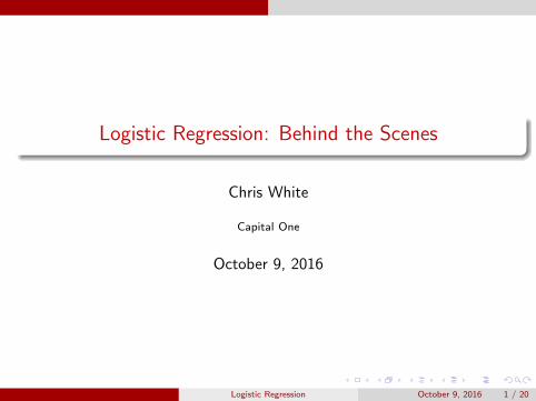
Generative Model
yi |β, xi ∼ Bernoulli(σ(β, xi )
)where
σ(β, x) :=1
1 + exp (−β · x)
is the sigmoid function.
Logistic Regression October 9, 2016 2 / 20
Outline Logistic Regression: A quick refresher
Interpretation
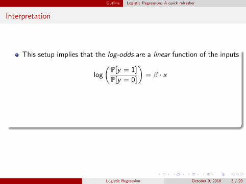
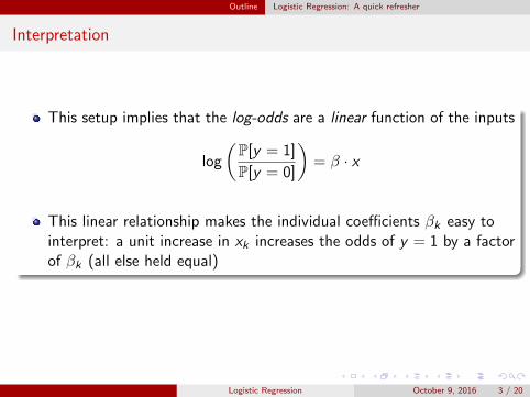
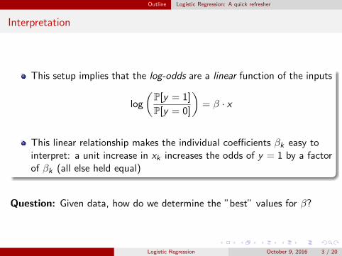
This setup implies that the log-odds are a linear function of the inputs
log
(P[y = 1]
P[y = 0]
)= β · x
This linear relationship makes the individual coefficients βk easy tointerpret: a unit increase in xk increases the odds of y = 1 by a factorof βk (all else held equal)
Question: Given data, how do we determine the ”best” values for β?
Logistic Regression October 9, 2016 3 / 20
Outline Logistic Regression: A quick refresher
Interpretation
This setup implies that the log-odds are a linear function of the inputs
log
(P[y = 1]
P[y = 0]
)= β · x
This linear relationship makes the individual coefficients βk easy tointerpret: a unit increase in xk increases the odds of y = 1 by a factorof βk (all else held equal)
Question: Given data, how do we determine the ”best” values for β?
Logistic Regression October 9, 2016 3 / 20
Outline Logistic Regression: A quick refresher
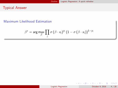
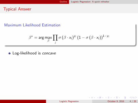
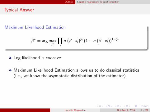
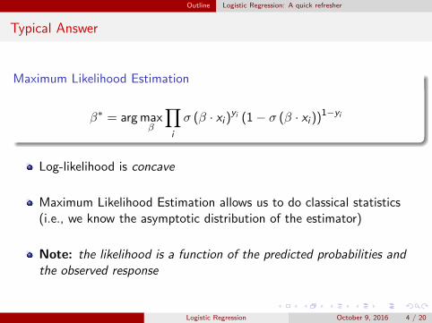
Typical Answer
Maximum Likelihood Estimation
β∗ = arg maxβ
∏i
σ (β · xi )yi (1− σ (β · xi ))1−yi
Log-likelihood is concave
Maximum Likelihood Estimation allows us to do classical statistics(i.e., we know the asymptotic distribution of the estimator)
Note: the likelihood is a function of the predicted probabilities andthe observed response
Logistic Regression October 9, 2016 4 / 20
Outline Logistic Regression: A quick refresher
Typical Answer
Maximum Likelihood Estimation
β∗ = arg maxβ
∏i
σ (β · xi )yi (1− σ (β · xi ))1−yi
Log-likelihood is concave
Maximum Likelihood Estimation allows us to do classical statistics(i.e., we know the asymptotic distribution of the estimator)
Note: the likelihood is a function of the predicted probabilities andthe observed response
Logistic Regression October 9, 2016 4 / 20
Outline This is not the end of the story
This is not the end of the story
Now we are confronted with an optimization problem...
The story doesn’t end here!
Uncritically throwing your data into an off-the-shelf solver could result in abad model.
Logistic Regression October 9, 2016 5 / 20
Outline This is not the end of the story
This is not the end of the story
Now we are confronted with an optimization problem...
The story doesn’t end here!
Uncritically throwing your data into an off-the-shelf solver could result in abad model.
Logistic Regression October 9, 2016 5 / 20

Outline This is not the end of the story
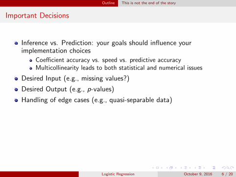
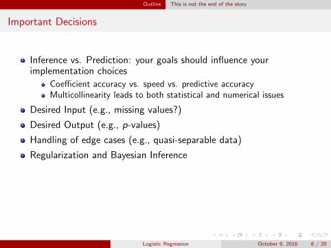
Important Decisions
Inference vs. Prediction: your goals should influence yourimplementation choices
Coefficient accuracy vs. speed vs. predictive accuracyMulticollinearity leads to both statistical and numerical issues
Desired Input (e.g., missing values?)
Desired Output (e.g., p-values)
Handling of edge cases (e.g., quasi-separable data)
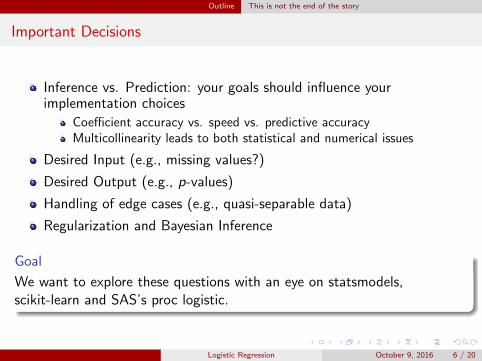
Regularization and Bayesian Inference
Goal
We want to explore these questions with an eye on statsmodels,scikit-learn and SAS’s proc logistic.
Logistic Regression October 9, 2016 6 / 20
Outline This is not the end of the story
Important Decisions
Inference vs. Prediction: your goals should influence yourimplementation choices
Coefficient accuracy vs. speed vs. predictive accuracyMulticollinearity leads to both statistical and numerical issues
Desired Input (e.g., missing values?)
Desired Output (e.g., p-values)
Handling of edge cases (e.g., quasi-separable data)
Regularization and Bayesian Inference
Goal
We want to explore these questions with an eye on statsmodels,scikit-learn and SAS’s proc logistic.
Logistic Regression October 9, 2016 6 / 20

Under the Hood How Needs Translate to Implementation Choices
Prediction vs. Inference
Coefficients and Convergence
In the case of inference, coefficient sign and precision are important.
Example: A model includes economic variables, and will be used for‘stress-testing‘ adverse economic scenarios.
Logistic Regression October 9, 2016 7 / 20
Under the Hood How Needs Translate to Implementation Choices
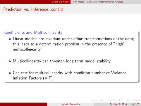
Prediction vs. Inference, cont’d
Coefficients and Multicollinearity
Linear models are invariant under affine transformations of the data;this leads to a determination problem in the presence of ”high”multicollinearity
Multicollinearity can threaten long term model stability
Can test for multicollinearity with condition number or VarianceInflation Factors (VIF)
Logistic Regression October 9, 2016 8 / 20
Under the Hood How Needs Translate to Implementation Choices
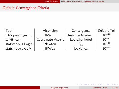
Default Convergence Criteria
Tool Algorithm Convergence Default Tol
SAS proc logistic IRWLS Relative Gradient 10−8
scikit-learn Coordinate Ascent Log-Likelihood 10−4
statsmodels Logit Newton `∞ 10−8
statsmodels GLM IRWLS Deviance 10−8
Note
Convergence criteria based on log-likelihood convergence emphasizeprediction stability.
Logistic Regression October 9, 2016 9 / 20
Under the Hood How Needs Translate to Implementation Choices
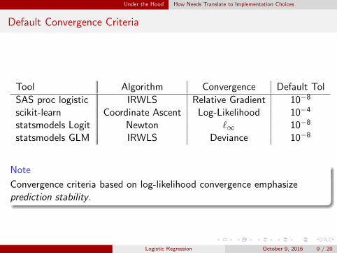
Default Convergence Criteria
Tool Algorithm Convergence Default Tol
SAS proc logistic IRWLS Relative Gradient 10−8
scikit-learn Coordinate Ascent Log-Likelihood 10−4
statsmodels Logit Newton `∞ 10−8
statsmodels GLM IRWLS Deviance 10−8
Note
Convergence criteria based on log-likelihood convergence emphasizeprediction stability.
Logistic Regression October 9, 2016 9 / 20
Under the Hood How Needs Translate to Implementation Choices
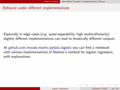
Behavior under different implementations
Especially in edge cases (e.g. quasi-separability, high multicollinearity)slightly different implementations can lead to drastically different outputs.
At github.com/moody-marlin/pydata logistic you can find a notebookwith various implementations of Newton’s method for logistic regression,with explanations.
Logistic Regression October 9, 2016 10 / 20

Under the Hood Input / Output
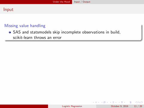
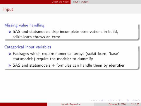
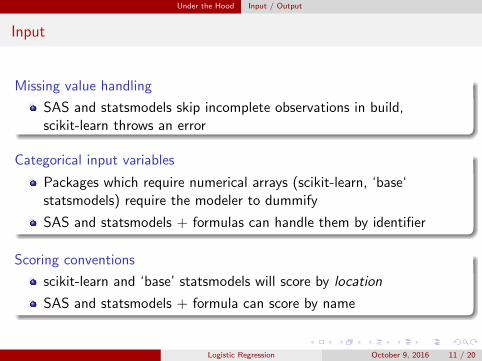
Input
Missing value handling
SAS and statsmodels skip incomplete observations in build,scikit-learn throws an error
Categorical input variables
Packages which require numerical arrays (scikit-learn, ‘base‘statsmodels) require the modeler to dummify
SAS and statsmodels + formulas can handle them by identifier
Scoring conventions
scikit-learn and ‘base’ statsmodels will score by location
SAS and statsmodels + formula can score by name
Logistic Regression October 9, 2016 11 / 20
Under the Hood Input / Output
Input
Missing value handling
SAS and statsmodels skip incomplete observations in build,scikit-learn throws an error
Categorical input variables
Packages which require numerical arrays (scikit-learn, ‘base‘statsmodels) require the modeler to dummify
SAS and statsmodels + formulas can handle them by identifier
Scoring conventions
scikit-learn and ‘base’ statsmodels will score by location
SAS and statsmodels + formula can score by name
Logistic Regression October 9, 2016 11 / 20

Under the Hood Input / Output
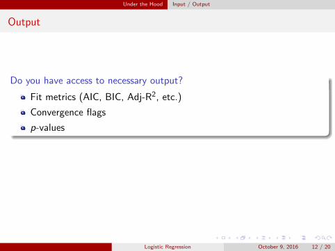
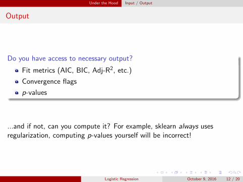
Output
Do you have access to necessary output?
Fit metrics (AIC, BIC, Adj-R2, etc.)
Convergence flags
p-values
...and if not, can you compute it? For example, sklearn always usesregularization, computing p-values yourself will be incorrect!
Logistic Regression October 9, 2016 12 / 20
Under the Hood Input / Output
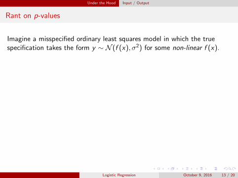
Rant on p-values
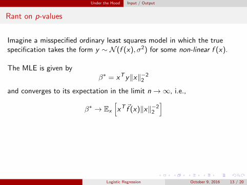
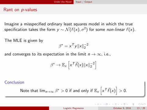
Imagine a misspecified ordinary least squares model in which the truespecification takes the form y ∼ N (f (x), σ2) for some non-linear f (x).
The MLE is given byβ∗ = xT y‖x‖−22
and converges to its expectation in the limit n→∞, i.e.,
β∗ → Ex
[xT ~f (x)‖x‖−22
]
Conclusion
Note that limn→∞ β∗ > 0 if and only if Ex
[xT ~f (x)
]> 0.
Logistic Regression October 9, 2016 13 / 20
Under the Hood Input / Output
Rant on p-values
Imagine a misspecified ordinary least squares model in which the truespecification takes the form y ∼ N (f (x), σ2) for some non-linear f (x).
The MLE is given byβ∗ = xT y‖x‖−22
and converges to its expectation in the limit n→∞, i.e.,
β∗ → Ex
[xT ~f (x)‖x‖−22
]
Conclusion
Note that limn→∞ β∗ > 0 if and only if Ex
[xT ~f (x)
]> 0.
Logistic Regression October 9, 2016 13 / 20

Under the Hood Input / Output
Rant on p-values
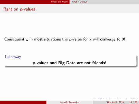
Consequently, in most situations the p-value for x will converge to 0!
Takeaway
p-values and Big Data are not friends!
Logistic Regression October 9, 2016 14 / 20
Under the Hood Input / Output
Rant on p-values
Consequently, in most situations the p-value for x will converge to 0!
Takeaway
p-values and Big Data are not friends!
Logistic Regression October 9, 2016 14 / 20
Regularization
Regularization
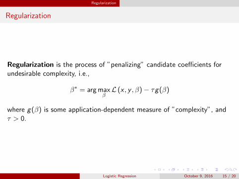
Regularization is the process of ”penalizing” candidate coefficients forundesirable complexity, i.e.,
β∗ = arg maxβL (x , y , β)− τg(β)
where g(β) is some application-dependent measure of ”complexity”, andτ > 0.
Logistic Regression October 9, 2016 15 / 20

Regularization
Regularization, cont’d
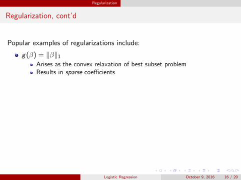
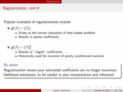
Popular examples of regularizations include:
g(β) = ‖β‖1
Arises as the convex relaxation of best subset problemResults in sparse coefficients
g(β) = ‖β‖22Results in ”ridged” coefficientsHistorically used for inversion of poorly conditioned matrices
Be aware
Regularization means your estimated coefficients are no longer maximumlikelihood estimators, so be careful in your interpretation and inference!
Logistic Regression October 9, 2016 16 / 20
Regularization
Regularization, cont’d
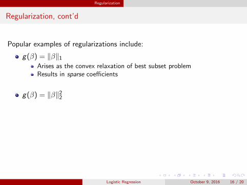
Popular examples of regularizations include:
g(β) = ‖β‖1Arises as the convex relaxation of best subset problemResults in sparse coefficients
g(β) = ‖β‖22Results in ”ridged” coefficientsHistorically used for inversion of poorly conditioned matrices
Be aware
Regularization means your estimated coefficients are no longer maximumlikelihood estimators, so be careful in your interpretation and inference!
Logistic Regression October 9, 2016 16 / 20
Regularization
Regularization, cont’d
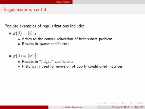
Popular examples of regularizations include:
g(β) = ‖β‖1Arises as the convex relaxation of best subset problemResults in sparse coefficients
g(β) = ‖β‖22
Results in ”ridged” coefficientsHistorically used for inversion of poorly conditioned matrices
Be aware
Regularization means your estimated coefficients are no longer maximumlikelihood estimators, so be careful in your interpretation and inference!
Logistic Regression October 9, 2016 16 / 20
Regularization
Regularization, cont’d
Popular examples of regularizations include:
g(β) = ‖β‖1Arises as the convex relaxation of best subset problemResults in sparse coefficients
g(β) = ‖β‖22Results in ”ridged” coefficientsHistorically used for inversion of poorly conditioned matrices
Be aware
Regularization means your estimated coefficients are no longer maximumlikelihood estimators, so be careful in your interpretation and inference!
Logistic Regression October 9, 2016 16 / 20
Regularization
Regularization, cont’d
Popular examples of regularizations include:
g(β) = ‖β‖1Arises as the convex relaxation of best subset problemResults in sparse coefficients
g(β) = ‖β‖22Results in ”ridged” coefficientsHistorically used for inversion of poorly conditioned matrices
Be aware
Regularization means your estimated coefficients are no longer maximumlikelihood estimators, so be careful in your interpretation and inference!
Logistic Regression October 9, 2016 16 / 20
Regularization
Caution!
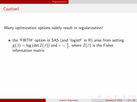
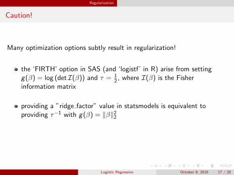
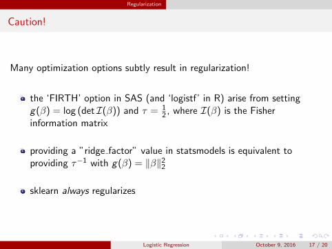
Many optimization options subtly result in regularization!
the ‘FIRTH’ option in SAS (and ‘logistf’ in R) arise from settingg(β) = log (det I(β)) and τ = 1
2 , where I(β) is the Fisherinformation matrix
providing a ”ridge factor” value in statsmodels is equivalent toproviding τ−1 with g(β) = ‖β‖22
sklearn always regularizes
Logistic Regression October 9, 2016 17 / 20
Regularization
Caution!
Many optimization options subtly result in regularization!
the ‘FIRTH’ option in SAS (and ‘logistf’ in R) arise from settingg(β) = log (det I(β)) and τ = 1
2 , where I(β) is the Fisherinformation matrix
providing a ”ridge factor” value in statsmodels is equivalent toproviding τ−1 with g(β) = ‖β‖22
sklearn always regularizes
Logistic Regression October 9, 2016 17 / 20
Regularization
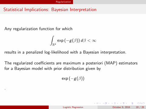
Statistical Implications: Bayesian Interpretation
Any regularization function for which∫Rk
exp (−g(β)) dβ <∞
results in a penalized log-likelihood with a Bayesian interpretation.
The regularized coefficients are maximum a posteriori (MAP) estimatorsfor a Bayesian model with prior distribution given by
exp (−g(β))
.
Logistic Regression October 9, 2016 18 / 20
Conclusion
Conclusion
Takeaway
Even if you don’t run into any edge cases, understanding what’s happeningunder the hood gives you access to much more information that you canleverage to build better, more informative models!
Logistic Regression October 9, 2016 19 / 20

THE END!
The End
Thanks for your time and attention! Questions?
Logistic Regression October 9, 2016 20 / 20
Top Related