


γλώσσες
Σελίδες
Νομικός

Lecture 6
Language Modeling/Pronunciation Modeling
Michael Picheny, Bhuvana Ramabhadran, Stanley F. Chen
IBM T.J. Watson Research CenterYorktown Heights, New York, USA
{picheny,bhuvana,stanchen}@us.ibm.com
15 October 2012
Review: Acoustic Modeling
x — Observations; sequence of ∼40d feature vectors.ω — word sequence.HMM/GMM framework lets us model P(x|ω) . . .
How likely feature vectors are given word sequence.
2 / 141
The Fundamental Equation of ASR
I HATE TO WAITEYE HATE TWO WEIGHT
ω∗ = arg maxω
P(x|ω)
⇓
ω∗ = arg maxω
P(ω|x) = arg maxω
P(ω)P(x|ω)
What’s new?Language model P(ω) describing . . .Frequency of each word sequence ω.
3 / 141
Part I
Language Modeling
4 / 141
Language Modeling: Goals
Describe which word sequences are likely.e.g., BRITNEY SPEARS vs. BRIT KNEE SPEARS.
Analogy: multiple-choice test.LM restricts choices given to acoustic model.The fewer choices, the better you do.
5 / 141
What Type of Model?
Want probability distribution over sequence of symbols.(Hidden) Markov model!Hidden or non-hidden?
For hidden, too hard to come up with topology.
6 / 141

Where Are We?
1 N-Gram Models
2 Technical Details
3 Smoothing
4 Discussion
7 / 141
What’s an n-Gram Model?
Markov model of order n − 1.To predict next word . . .
Only need to remember last n − 1 words.
8 / 141
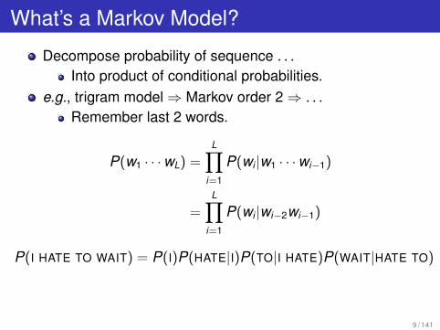
What’s a Markov Model?
Decompose probability of sequence . . .Into product of conditional probabilities.
e.g., trigram model ⇒ Markov order 2 ⇒ . . .Remember last 2 words.
P(w1 · · ·wL) =L∏
i=1
P(wi |w1 · · ·wi−1)
=L∏
i=1
P(wi |wi−2wi−1)
P(I HATE TO WAIT) = P(I)P(HATE|I)P(TO|I HATE)P(WAIT|HATE TO)
9 / 141

Sentence Begins and Ends
Pad left with beginning-of-sentence tokens.e.g., w−1 = w0 = ..Always condition on two words to left, even at start.
Predict end-of-sentence token at end.So true probability, i.e.,
∑ω P(ω) = 1.
P(w1 · · ·wL) =L+1∏i=1
P(wi |wi−2wi−1)
P(I HATE TO WAIT) = P(I| . .)× P(HATE| . I)× P(TO|I HATE)×P(WAIT|HATE TO)× P(/|TO WAIT)
10 / 141
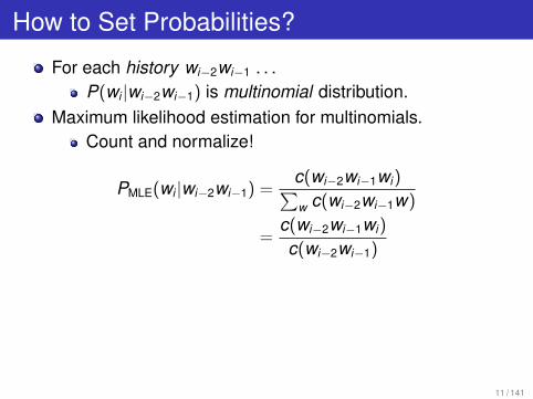
How to Set Probabilities?
For each history wi−2wi−1 . . .P(wi |wi−2wi−1) is multinomial distribution.
Maximum likelihood estimation for multinomials.Count and normalize!
PMLE(wi |wi−2wi−1) =c(wi−2wi−1wi)∑w c(wi−2wi−1w)
=c(wi−2wi−1wi)
c(wi−2wi−1)
11 / 141
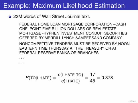
Example: Maximum Likelihood Estimation
23M words of Wall Street Journal text.
FEDERAL HOME LOAN MORTGAGE CORPORATION –DASHONE .POINT FIVE BILLION DOLLARS OF REALESTATEMORTGAGE -HYPHEN INVESTMENT CONDUIT SECURITIESOFFERED BY MERRILL LYNCH &ERSAND COMPANY
NONCOMPETITIVE TENDERS MUST BE RECEIVED BY NOONEASTERN TIME THURSDAY AT THE TREASURY OR ATFEDERAL RESERVE BANKS OR BRANCHES. . .. . .
P(TO|I HATE) =c(I HATE TO)
c(I HATE)=
1745
= 0.378
12 / 141
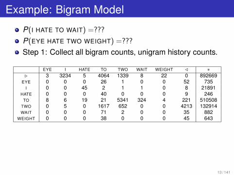
Example: Bigram Model
P(I HATE TO WAIT) =???
P(EYE HATE TWO WEIGHT) =???
Step 1: Collect all bigram counts, unigram history counts.
EYE I HATE TO TWO WAIT WEIGHT / ∗. 3 3234 5 4064 1339 8 22 0 892669
EYE 0 0 0 26 1 0 0 52 735I 0 0 45 2 1 1 0 8 21891
HATE 0 0 0 40 0 0 0 9 246TO 8 6 19 21 5341 324 4 221 510508
TWO 0 5 0 1617 652 0 0 4213 132914WAIT 0 0 0 71 2 0 0 35 882
WEIGHT 0 0 0 38 0 0 0 45 643
13 / 141
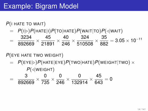
Example: Bigram Model
P(I HATE TO WAIT)
= P(I|.)P(HATE|I)P(TO|HATE)P(WAIT|TO)P(/|WAIT)
=3234
892669× 45
21891× 40
246× 324
510508× 35
882= 3.05× 10⁻¹¹
P(EYE HATE TWO WEIGHT)
= P(EYE|.)P(HATE|EYE)P(TWO|HATE)P(WEIGHT|TWO)×P(/|WEIGHT)
=3
892669× 0
735× 0
246× 0
132914× 45
643= 0
14 / 141

Recap: N-Gram Models
Simple formalism, yet effective.Discriminates between wheat and chaff.
Easy to train: count and normalize.Generalizes.
Assigns nonzero probabilities to sentences . . .Not seen in training data, e.g., I HATE TO WAIT.
15 / 141

Where Are We?
1 N-Gram Models
2 Technical Details
3 Smoothing
4 Discussion
16 / 141
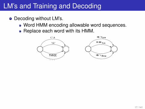
LM’s and Training and Decoding
Decoding without LM’s.Word HMM encoding allowable word sequences.Replace each word with its HMM.
ONE
TWO
THREE
. . . . . .
HMMone
HMMtwo
HMMthree
. . . . . .
17 / 141
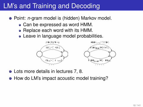
LM’s and Training and Decoding
Point: n-gram model is (hidden) Markov model.Can be expressed as word HMM.Replace each word with its HMM.Leave in language model probabilities.
ONE/P(ONE)
TWO/P(TWO)
THREE/P(THREE)
. . . . . .
HMMone/P(ONE)
HMMtwo/P(TWO)
HMMthree/P(THREE)
. . . . . . . . .
Lots more details in lectures 7, 8.How do LM’s impact acoustic model training?
18 / 141
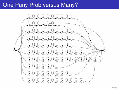
One Puny Prob versus Many?
one
two
three
four
�ve
six
seveneight
nine
zero
19 / 141
The Acoustic Model Weight
Not a fair fight.Solution: acoustic model weight.
ω∗ = arg maxω
P(ω)P(x|ω)α
α usually somewhere between 0.05 and 0.1.Important to tune for each LM, AM.Theoretically inelegant.
Empirical performance trumps theory any day of week.Is it LM weight or AM weight?
20 / 141
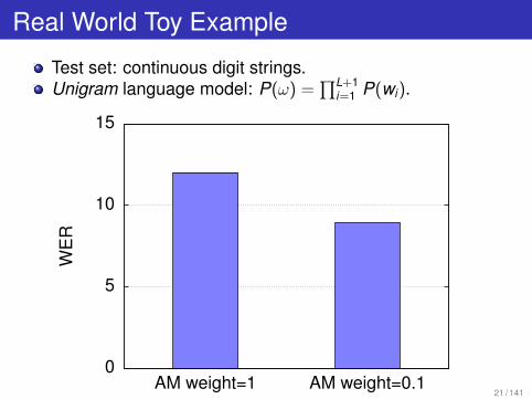
Real World Toy Example
Test set: continuous digit strings.Unigram language model: P(ω) =
∏L+1i=1 P(wi).
0
5
10
15
AM weight=1 AM weight=0.1
WE
R
21 / 141
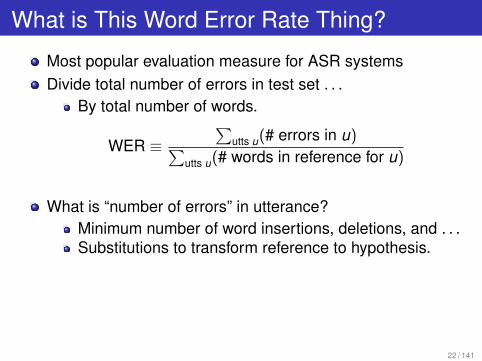
What is This Word Error Rate Thing?
Most popular evaluation measure for ASR systemsDivide total number of errors in test set . . .
By total number of words.
WER ≡∑
utts u(# errors in u)∑utts u(# words in reference for u)
What is “number of errors” in utterance?Minimum number of word insertions, deletions, and . . .Substitutions to transform reference to hypothesis.
22 / 141
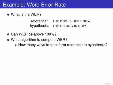
Example: Word Error Rate
What is the WER?
reference: THE DOG IS HERE NOWhypothesis: THE UH BOG IS NOW
Can WER be above 100%?What algorithm to compute WER?
How many ways to transform reference to hypothesis?
23 / 141
Evaluating Language Models
Best way: plug into ASR system; measure WER.Need ASR system.Expensive to compute (especially in old days).Results depend on acoustic model.
Is there something cheaper that predicts WER well?
24 / 141
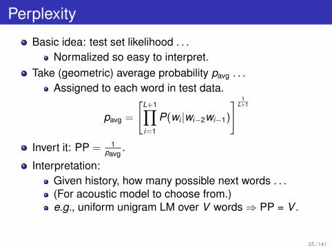
Perplexity
Basic idea: test set likelihood . . .Normalized so easy to interpret.
Take (geometric) average probability pavg . . .Assigned to each word in test data.
pavg =
[L+1∏i=1
P(wi |wi−2wi−1)
] 1L+1
Invert it: PP = 1pavg
.
Interpretation:Given history, how many possible next words . . .(For acoustic model to choose from.)e.g., uniform unigram LM over V words ⇒ PP = V .
25 / 141
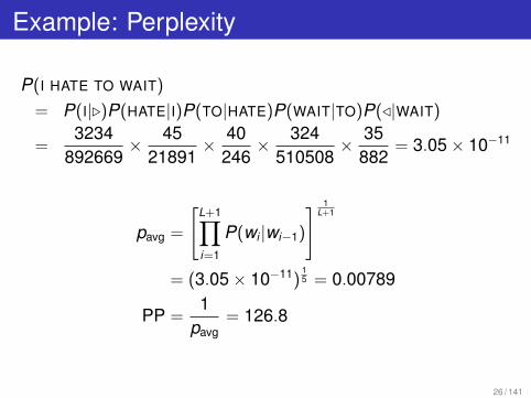
Example: Perplexity
P(I HATE TO WAIT)
= P(I|.)P(HATE|I)P(TO|HATE)P(WAIT|TO)P(/|WAIT)
=3234
892669× 45
21891× 40
246× 324
510508× 35
882= 3.05× 10⁻¹¹
pavg =
[L+1∏i=1
P(wi |wi−1)
] 1L+1
= (3.05× 10⁻¹¹)15 = 0.00789
PP =1
pavg= 126.8
26 / 141
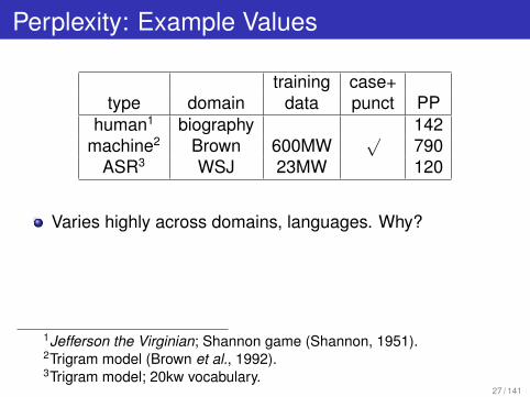
Perplexity: Example Values
training case+type domain data punct PP
human1 biography 142machine2 Brown 600MW
√790
ASR3 WSJ 23MW 120
Varies highly across domains, languages. Why?
1Jefferson the Virginian; Shannon game (Shannon, 1951).2Trigram model (Brown et al., 1992).3Trigram model; 20kw vocabulary.
27 / 141
Does Perplexity Predict Word-Error Rate?
Not across different LM types.e.g., word n-gram model; class n-gram model; . . .
OK within LM type.e.g., vary training set; model order; pruning; . . .
28 / 141
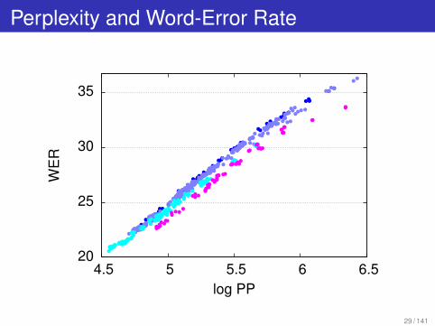
Perplexity and Word-Error Rate
20
25
30
35
4.5 5 5.5 6 6.5
WE
R
log PP
29 / 141
Recap
LM describes allowable word sequences.Used to build decoding graph.
Need AM weight for LM to have full effect.Best to evaluate LM’s using WER . . .
But perplexity can be informative.Can you think of any problems with word error rate?
What do we really care about in applications?
30 / 141

Where Are We?
1 N-Gram Models
2 Technical Details
3 Smoothing
4 Discussion
31 / 141

An Experiment
Take 50M words of WSJ; shuffle sentences; split in two.“Training” set: 25M words.
NONCOMPETITIVE TENDERS MUST BE RECEIVED BY NOONEASTERN TIME THURSDAY AT THE TREASURY OR ATFEDERAL RESERVE BANKS OR BRANCHES .PERIOD
NOT EVERYONE AGREED WITH THAT STRATEGY .PERIOD. . .. . .
“Test” set: 25M words.NATIONAL PICTURE &ERSAND FRAME –DASH INITIALTWO MILLION ,COMMA TWO HUNDRED FIFTY THOUSANDSHARES ,COMMA VIA WILLIAM BLAIR .PERIOD
THERE WILL EVEN BE AN EIGHTEEN -HYPHEN HOLE GOLFCOURSE .PERIOD. . .. . .
32 / 141
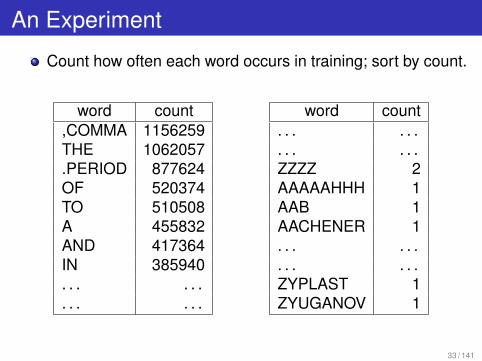
An Experiment
Count how often each word occurs in training; sort by count.
word count,COMMA 1156259THE 1062057.PERIOD 877624OF 520374TO 510508A 455832AND 417364IN 385940. . . . . .. . . . . .
word count. . . . . .. . . . . .ZZZZ 2AAAAAHHH 1AAB 1AACHENER 1. . . . . .. . . . . .ZYPLAST 1ZYUGANOV 1
33 / 141
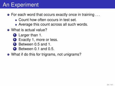
An Experiment
For each word that occurs exactly once in training . . .Count how often occurs in test set.Average this count across all such words.
What is actual value?1 Larger than 1.2 Exactly 1, more or less.3 Between 0.5 and 1.4 Between 0.1 and 0.5.
What if do this for trigrams, not unigrams?
34 / 141

Why?
Q: How many unigrams/trigrams in test set . . .Do not appear in training set?A: 48k/7.4M.
Q: How many unique unigrams/trigrams in training set?A: 135k/9.4M.
On average, everything seen in training is discounted!
35 / 141
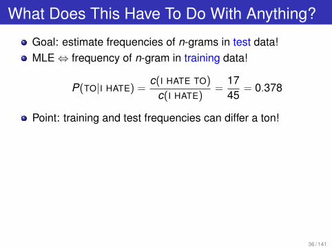
What Does This Have To Do With Anything?
Goal: estimate frequencies of n-grams in test data!MLE ⇔ frequency of n-gram in training data!
P(TO|I HATE) =c(I HATE TO)
c(I HATE)=
1745
= 0.378
Point: training and test frequencies can differ a ton!
36 / 141
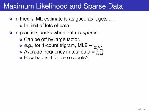
Maximum Likelihood and Sparse Data
In theory, ML estimate is as good as it gets . . .In limit of lots of data.
In practice, sucks when data is sparse.Can be off by large factor.e.g., for 1-count trigram, MLE = 1
25M .Average frequency in test data = 0.25
25M .How bad is it for zero counts?
37 / 141
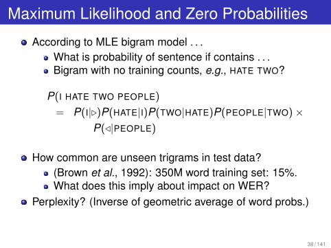
Maximum Likelihood and Zero Probabilities
According to MLE bigram model . . .What is probability of sentence if contains . . .Bigram with no training counts, e.g., HATE TWO?
P(I HATE TWO PEOPLE)
= P(I|.)P(HATE|I)P(TWO|HATE)P(PEOPLE|TWO)×P(/|PEOPLE)
How common are unseen trigrams in test data?(Brown et al., 1992): 350M word training set: 15%.What does this imply about impact on WER?
Perplexity? (Inverse of geometric average of word probs.)
38 / 141
Smoothing
Adjusting ML estimates to better match test data.How to decrease probabilities for seen stuff?How to estimate probabilities for unseen stuff?
Also called regularization.
39 / 141
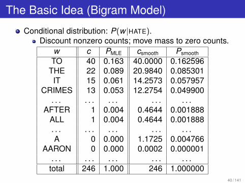
The Basic Idea (Bigram Model)
Conditional distribution: P(w |HATE).Discount nonzero counts; move mass to zero counts.
w c PMLE csmooth Psmooth
TO 40 0.163 40.0000 0.162596THE 22 0.089 20.9840 0.085301IT 15 0.061 14.2573 0.057957
CRIMES 13 0.053 12.2754 0.049900. . . . . . . . . . . . . . .
AFTER 1 0.004 0.4644 0.001888ALL 1 0.004 0.4644 0.001888. . . . . . . . . . . . . . .A 0 0.000 1.1725 0.004766
AARON 0 0.000 0.0002 0.000001. . . . . . . . . . . . . . .
total 246 1.000 246 1.00000040 / 141
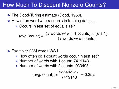
How Much To Discount Nonzero Counts?
The Good-Turing estimate (Good, 1953).How often word with k counts in training data . . .
Occurs in test set of equal size?
(avg. count) ≈ (# words w/ k + 1 counts)× (k + 1)
(# words w/ k counts)
Example: 23M words WSJ.How often do 1-count words occur in test set?Number of words with 1 count: 7419143.Number of words with 2 counts: 933493.
(avg. count) ≈ 933493× 27419143
= 0.252
41 / 141
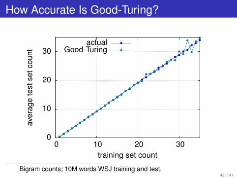
How Accurate Is Good-Turing?
0
10
20
30
0 10 20 30
aver
age
test
setc
ount
training set count
actualGood-Turing
Bigram counts; 10M words WSJ training and test.42 / 141
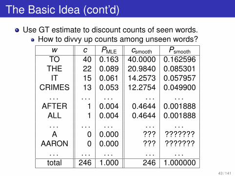
The Basic Idea (cont’d)
Use GT estimate to discount counts of seen words.How to divvy up counts among unseen words?
w c PMLE csmooth Psmooth
TO 40 0.163 40.0000 0.162596THE 22 0.089 20.9840 0.085301IT 15 0.061 14.2573 0.057957
CRIMES 13 0.053 12.2754 0.049900. . . . . . . . . . . . . . .
AFTER 1 0.004 0.4644 0.001888ALL 1 0.004 0.4644 0.001888. . . . . . . . . . . . . . .A 0 0.000 ??? ???????
AARON 0 0.000 ??? ???????. . . . . . . . . . . . . . .
total 246 1.000 246 1.00000043 / 141
Backoff
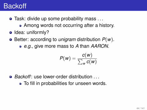
Task: divide up some probability mass . . .Among words not occurring after a history.
Idea: uniformly?Better: according to unigram distribution P(w).
e.g., give more mass to A than AARON.
P(w) =c(w)∑w c(w)
Backoff : use lower-order distribution . . .To fill in probabilities for unseen words.
44 / 141
Putting It All Together: Katz Smoothing
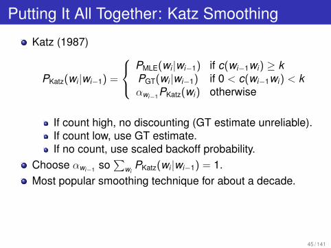
Katz (1987)
PKatz(wi |wi−1) =
PMLE(wi |wi−1) if c(wi−1wi) ≥ kPGT(wi |wi−1) if 0 < c(wi−1wi) < kαwi−1PKatz(wi) otherwise
If count high, no discounting (GT estimate unreliable).If count low, use GT estimate.If no count, use scaled backoff probability.
Choose αwi−1 so∑
wiPKatz(wi |wi−1) = 1.
Most popular smoothing technique for about a decade.
45 / 141
Example: Katz Smoothing
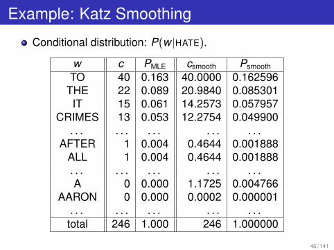
Conditional distribution: P(w |HATE).
w c PMLE csmooth Psmooth
TO 40 0.163 40.0000 0.162596THE 22 0.089 20.9840 0.085301IT 15 0.061 14.2573 0.057957
CRIMES 13 0.053 12.2754 0.049900. . . . . . . . . . . . . . .
AFTER 1 0.004 0.4644 0.001888ALL 1 0.004 0.4644 0.001888. . . . . . . . . . . . . . .A 0 0.000 1.1725 0.004766
AARON 0 0.000 0.0002 0.000001. . . . . . . . . . . . . . .
total 246 1.000 246 1.000000
46 / 141
Recap: Smoothing
ML estimates: way off for low counts.Zero probabilities kill performance.
Key aspects of smoothing algorithms.How to discount counts of seen words.Estimating mass of unseen words.Backoff to get information from lower-order models.
No downside.
47 / 141

Where Are We?
1 N-Gram Models
2 Technical Details
3 Smoothing
4 Discussion
48 / 141
N-Gram Models
Workhorse of language modeling for ASR for 30 years.Used in great majority of deployed systems.
Almost no linguistic knowledge.Totally data-driven.
Easy to build.Fast and scalable.Can train on vast amounts of data; just gets better.
49 / 141
Smoothing
Lots and lots of smoothing algorithms developed.Will talk about newer algorithms in Lecture 11.Gain: ∼1% absolute in WER over Katz.
With good smoothing, don’t worry models being too big!Can increase n-gram order w/o loss in performance.Can gain in performance if lots of data.
Rule of thumb: if ML estimate is working OK . . .Model is way too small.
50 / 141
Does Markov Property Hold For English?
Not for small n.
P(wi | OF THE) 6= P(wi | KING OF THE)
Make n larger?FABIO, WHO WAS NEXT IN LINE, ASKED IF THETELLER SPOKE . . .Lots more to say about language modeling . . .
In Lecture 11.
51 / 141

References
C.E. Shannon, “Prediction and Entropy of Printed English”,Bell Systems Technical Journal, vol. 30, pp. 50–64, 1951.
I.J. Good, “The Population Frequencies of Species and theEstimation of Population Parameters”, Biometrika, vol. 40,no. 3 and 4, pp. 237–264, 1953.
S.M. Katz, “Estimation of Probabilities from Sparse Data forthe Language Model Component of a Speech Recognizer”,IEEE Transactions on Acoustics, Speech and SignalProcessing, vol. 35, no. 3, pp. 400–401, 1987.
P.F. Brown, S.A. Della Pietra, V.J. Della Pietra, J.C. Lai, R.L.Mercer, “An Estimate of an Upper Bound for the Entropy ofEnglish”, Computational Linguistics, vol. 18, no. 1, pp.31–40, 1992.
52 / 141

Part II
Administrivia
53 / 141
Administrivia
Clear (7); mostly clear (10); unclear (1).Pace: too fast/too much content (4); OK (10); too slow/notenough time on LM’s (2).Feedback (2+ votes):
More demos (2).More examples (2).Post answers to lab/sooner (2).Put administrivia in middle of lecture.
Muddiest: n-grams (2); . . .
54 / 141

Administrivia
Lab 1Handed back today?Answers:/user1/faculty/stanchen/e6870/lab1_ans/
Lab 2Due two days from now (Wednesday, Oct. 17) at 6pm.Xiao-Ming has extra office hours: Tue 2-4pm.
Optional non-reading projects.Will be posted Thursday; we’ll send out announcement.Proposal will be due week from Wednesday (Oct. 24).For reading projects, oral presentation ⇒ paper.
55 / 141
Part III
Pronunciation Modeling
56 / 141
In the beginning...
... . was the whole word model.For each word in the vocabulary, decide on a topology.Often the number of states in the model is chosen to beproportional to the number of phonemes in the word.Train the observation and transition parameters for a givenword using examples of that word in the training data.Good domain for this approach: digits.
57 / 141
Example topologies: Digits
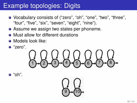
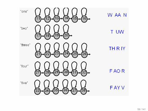
Vocabulary consists of (“zero”, “oh”, “one”, “two”, “three”,“four”, “five”, “six”, “seven”, “eight”, “nine”).Assume we assign two states per phoneme.Must allow for different durationsModels look like:“zero”.
“oh”.
58 / 141
59 / 141
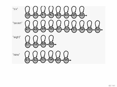
60 / 141
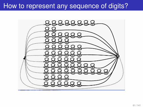
How to represent any sequence of digits?
61 / 141
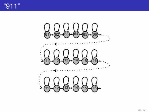
“911”
62 / 141
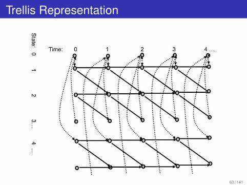
Trellis Representation
63 / 141
Whole-word model limitations
The whole-word model suffers from two main problems.Cannot model unseen words. In fact, we need severalsamples of each word to train the models properly.Cannot share data among models – data sparsenessproblem.The number of parameters in the system isproportional to the vocabulary size.
Thus, whole-word models are best on small vocabularytasks.
64 / 141
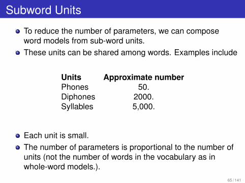
Subword Units
To reduce the number of parameters, we can composeword models from sub-word units.These units can be shared among words. Examples include
Units Approximate numberPhones 50.Diphones 2000.Syllables 5,000.
Each unit is small.The number of parameters is proportional to the number ofunits (not the number of words in the vocabulary as inwhole-word models.).
65 / 141
Phonetic Models
We represent each word as a sequence of phonemes. Thisrepresentation is the “baseform” for the word.
BANDS -> B AE N D Z
Some words need more than one baseform.
THE -> DH UH-> DH IY
66 / 141
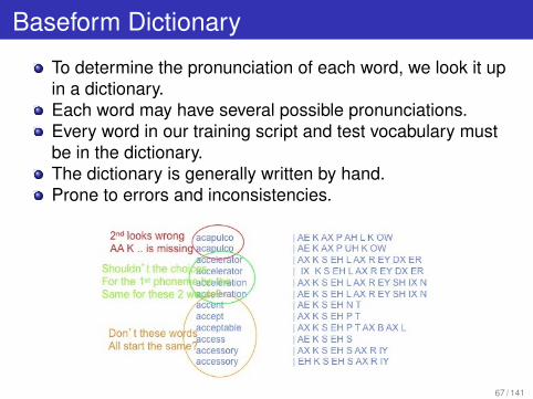
Baseform Dictionary
To determine the pronunciation of each word, we look it upin a dictionary.Each word may have several possible pronunciations.Every word in our training script and test vocabulary mustbe in the dictionary.The dictionary is generally written by hand.Prone to errors and inconsistencies.
67 / 141
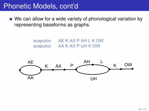
Phonetic Models, cont’d
We can allow for a wide variety of phonological variation byrepresenting baseforms as graphs.
68 / 141
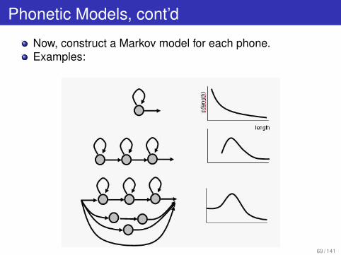
Phonetic Models, cont’d
Now, construct a Markov model for each phone.Examples:
69 / 141
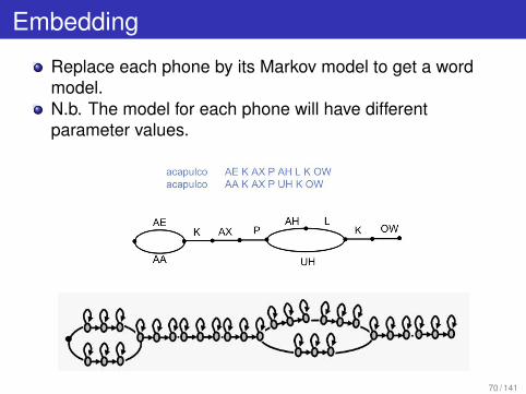
Embedding
Replace each phone by its Markov model to get a wordmodel.N.b. The model for each phone will have differentparameter values.
70 / 141
Reducing Parameters by Tying
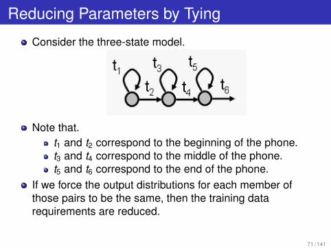
Consider the three-state model.
Note that.t1 and t2 correspond to the beginning of the phone.t3 and t4 correspond to the middle of the phone.t5 and t6 correspond to the end of the phone.
If we force the output distributions for each member ofthose pairs to be the same, then the training datarequirements are reduced.
71 / 141
Tying
A set of arcs in a Markov model are tied to one another ifthey are constrained to have identical output distributions.Similarly, states are tied if they have identical transitionprobabilities.Tying can be explicit or implicit.
72 / 141
Implicit Tying
Occurs when we build up models for larger units frommodels of smaller units.Example: when word models are made from phone models.First, consider an example without any tying.
Let the vocabulary consist of digits 0,1,2,... 9.We can make a separate model for each word.To estimate parameters for each word model, we needseveral samples for each word.Samples of “0” affect only parameters for the “0” model.
73 / 141
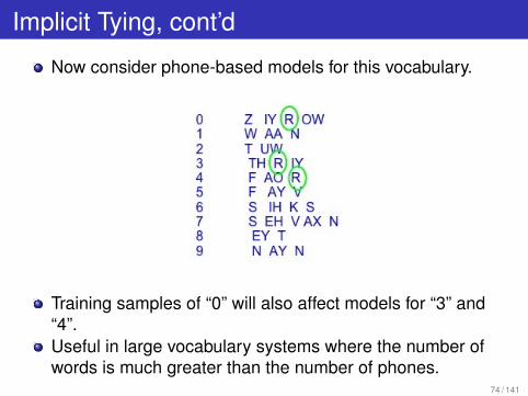
Implicit Tying, cont’d
Now consider phone-based models for this vocabulary.
Training samples of “0” will also affect models for “3” and“4”.Useful in large vocabulary systems where the number ofwords is much greater than the number of phones.
74 / 141

Explicit Tying
Example:
6 non-null arcs, but only 3 different output distributionsbecause of tying.Number of model parameters is reduced.Tying saves storage because only one copy of eachdistribution is saved.Fewer parameters mean less training data needed.
75 / 141
Variations in realizations of phonemes
The broad units, phonemes, have variants known asallophones
Example: p and ph (un-aspirated and aspirated p).Exercise: Put your hand in front of your mouth andpronounce spin and then pin Note that the p in pin hasa puff of air,. while the p in spin does not.
Articulators have inertia, thus the pronunciation of aphoneme is influenced by surrounding phonemes. This isknown as co-articulation
Example: Consider k and g in different contexts.In key and geese the whole body of the tongue has to bepulled up to make the vowel.Closure of the k moves forward compared to caw and gauze.
Phonemes have canonical articulator target positions thatmay or may not be reached in a particular utterance.
76 / 141
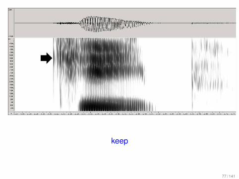
keep
77 / 141
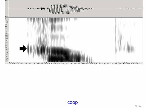
coop78 / 141
Context-dependent models
We can model phones in context.Two approaches: “triphones” and "Decision Trees".Both methods use clustering. “Triphones” use bottom-upclustering, "Decision trees" implement top-down clustering.Typical improvements of speech recognizers whenintroducing context dependence: 30% - 50% fewer errors.
79 / 141
Triphone models
Model each phoneme in the context of its left and rightneighbor.E.g. K-IY+P is a model for IY when K is its left contextphoneme and P is its right context phoneme.If we have 50 phonemes in a language, we could have asmany as 503 triphones to model.Not all of these occur.Still have data sparsity issues.Try to solve these issues by agglomerative clustering.
80 / 141
Agglomerative / “Bottom-up” Clustering
Start with each item in a cluster by itself.Find “closest” pair of items.Merge them into a single cluster.Iterate.Different results based on distance measure used.
Single-link: dist(A,B) = min dist(a,b) for aA, bB.Complete-link: dist(A,B) = max dist(a,b) for aA, bB.
81 / 141
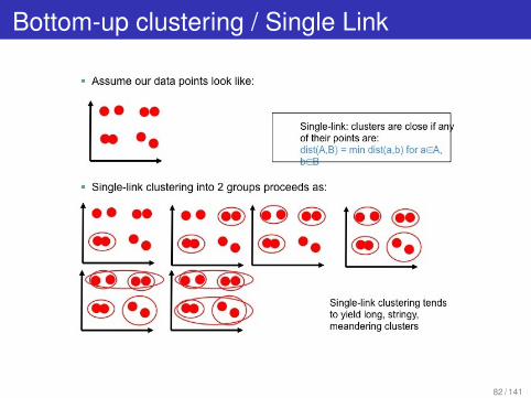
Bottom-up clustering / Single Link
82 / 141
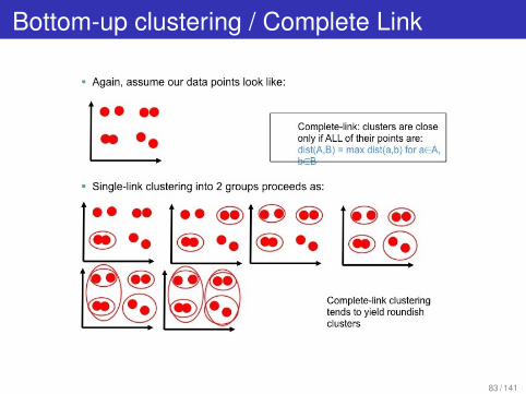
Bottom-up clustering / Complete Link
83 / 141
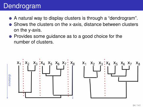
Dendrogram
A natural way to display clusters is through a “dendrogram”.Shows the clusters on the x-axis, distance between clusterson the y-axis.Provides some guidance as to a good choice for thenumber of clusters.
84 / 141
Triphone Clustering
We can use e.g. complete-link clustering to clustertriphones.Helps with data sparsity issue.Still have an issue with unseen data.To model unseen events, we need to “back-off” to lowerorder models such as bi-phones and uni-phones.
85 / 141
Decision Trees
Goal of any clustering scheme is to find equivalenceclasses among our training samples.A decision tree maps data tagged with set of input variablesinto equivalence classes.Asks questions about the input variables to designed toimprove some criterion function associated with the trainingdata.
Output data may be labels - criteria could be entropyOutput data may be real numbers or vector - criteriacould be mean-square error
The goal when constructing a decision tree is significantlyimprove the criterion function (relative to doing nothing)
86 / 141
Decision Trees - A Form of Top-DownClustering
DTs perform top-down clustering because constructed byasking series of questions that recursively split the trainingdata.In our case,
The input features will be phonetic context (the phonesto left and right of phone for which we are creating acontext-dependent model;The output data will be the feature vectors associatedwith each phoneThe criterion function will be the likelihood of the outputfeatures.
Classic text: L. Breiman et al. Classification andRegression Trees. Wadsworth & Brooks. Monterey,California. 1984.
87 / 141
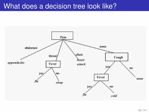
What does a decision tree look like?
88 / 141

Types of Input Attributes/Features
Numerical: Domain is ordered and can be represented onthe real line (e.g., age, income).Nominal or categorical: Domain is a finite set without anynatural ordering (e.g., occupation, marital status, race).Ordinal: Domain is ordered, but absolute differencesbetween values is unknown (e.g., preference scale, severityof an injury).
89 / 141
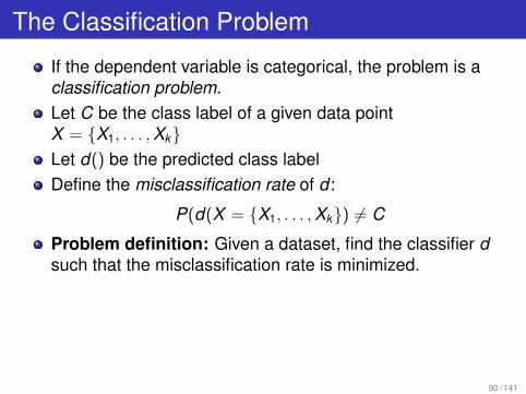
The Classification Problem
If the dependent variable is categorical, the problem is aclassification problem.Let C be the class label of a given data pointX = {X1, . . . , Xk}Let d() be the predicted class labelDefine the misclassification rate of d :
P(d(X = {X1, . . . , Xk}) 6= C
Problem definition: Given a dataset, find the classifier dsuch that the misclassification rate is minimized.
90 / 141
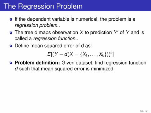
The Regression Problem
If the dependent variable is numerical, the problem is aregression problem..The tree d maps observation X to prediction Y ′ of Y and iscalled a regression function..Define mean squared error of d as:
E [(Y − d(X = {X1, . . . , Xk}))2]
Problem definition: Given dataset, find regression functiond such that mean squared error is minimized.
91 / 141
Goals & Requirements
Traditional Goals of Decision TreesTo produce an accurate classifier/regression function.To understand the structure of the problem.
Traditional Requirements on the model:High accuracy.Understandable by humans, interpretable.Fast construction for very large training databases.
For speech recognition, understandibility quickly goes outthe window....
92 / 141
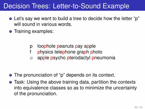
Decision Trees: Letter-to-Sound Example
Let’s say we want to build a tree to decide how the letter “p”will sound in various words.Training examples:
p loophole peanuts pay applef physics telephone graph photoφ apple psycho pterodactyl pneumonia
The pronunciation of “p” depends on its context.Task: Using the above training data, partition the contextsinto equivalence classes so as to minimize the uncertaintyof the pronunciation.
93 / 141
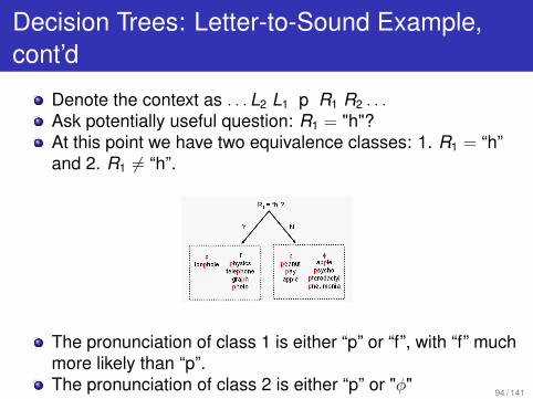
Decision Trees: Letter-to-Sound Example,cont’d
Denote the context as . . . L2 L1 p R1 R2 . . .Ask potentially useful question: R1 = "h"?At this point we have two equivalence classes: 1. R1 = “h”and 2. R1 6= “h”.
The pronunciation of class 1 is either “p” or “f”, with “f” muchmore likely than “p”.The pronunciation of class 2 is either “p” or "φ"
94 / 141

Four equivalence classes. Uncertainty only remains in class 3.
95 / 141
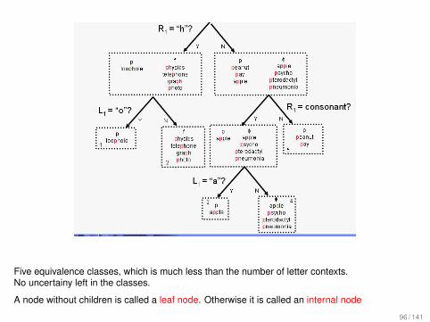
Five equivalence classes, which is much less than the number of letter contexts.No uncertainy left in the classes.
A node without children is called a leaf node. Otherwise it is called an internal node
96 / 141
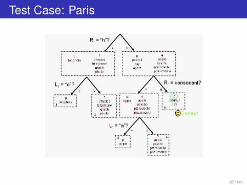
Test Case: Paris
97 / 141
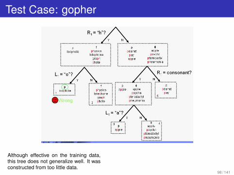
Test Case: gopher
Although effective on the training data,this tree does not generalize well. It wasconstructed from too little data.
98 / 141

Decision Tree Construction
1 Find the best question for partitioning the data at a givennode into 2 equivalence classes.
2 Repeat step 1 recursively on each child node.3 Stop when there is insufficient data to continue or when the
best question is not sufficiently helpful.
99 / 141
Basic Issues to Solve
The selection of the splits.The decisions when to declare a node terminal or tocontinue splitting.
100 / 141
Decision Tree Construction – FundamentalOperation
There is only 1 fundamental operation in tree construction:Find the best question for partitioning a subset of thedata into two smaller subsets.i.e. Take an equivalence class and split it into 2more-specific classes.
101 / 141
Decision Tree Greediness
Tree construction proceeds from the top down – from root toleaf.Each split is intended to be locally optimal.Constructing a tree in this “greedy” fashion usually leads toa good tree, but probably not globally optimal.Finding the globally optimal tree is an NP-completeproblem: it is not practical.
102 / 141
Splitting
Each internal node has an associated splitting question.Example questions:
Age <= 20 (numeric).Profession in (student, teacher) (categorical).5000*Age + 3*Salary – 10000 > 0 (function of rawfeatures).
103 / 141
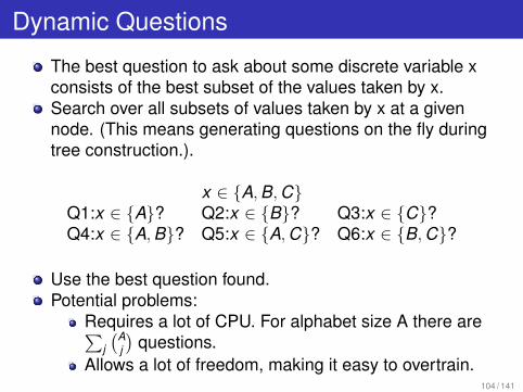
Dynamic Questions
The best question to ask about some discrete variable xconsists of the best subset of the values taken by x.Search over all subsets of values taken by x at a givennode. (This means generating questions on the fly duringtree construction.).
x ∈ {A, B, C}Q1:x ∈ {A}? Q2:x ∈ {B}? Q3:x ∈ {C}?Q4:x ∈ {A, B}? Q5:x ∈ {A, C}? Q6:x ∈ {B, C}?
Use the best question found.Potential problems:
Requires a lot of CPU. For alphabet size A there are∑j
(Aj
)questions.
Allows a lot of freedom, making it easy to overtrain.104 / 141
Pre-determined Questions
The easiest way to construct a decision tree is to create inadvance a list of possible questions for each variable.Finding the best question at any given node consists ofsubjecting all relevant variables to each of the questions,and picking the best combination of variable and question.In acoustic modeling, we typically ask about 2-4 variables:the 1-2 phones to the left of the current phone and the 1-2phones to the right of the current phone. Since thesevariables all span the same alphabet (phone alphabet) onlyone list of questions.Each question on this list consists of a subset of thephonetic phone alphabet.
105 / 141
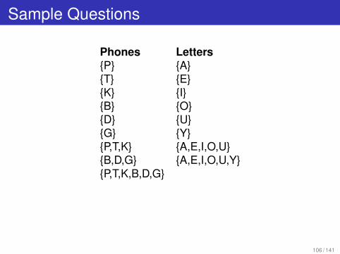
Sample Questions
Phones Letters{P} {A}{T} {E}{K} {I}{B} {O}{D} {U}{G} {Y}{P,T,K} {A,E,I,O,U}{B,D,G} {A,E,I,O,U,Y}{P,T,K,B,D,G}
106 / 141
Discrete Questions
A decision tree has a question associated with everynon-terminal node.If x is a discrete variable which takes on values in somefinite alphabet A, then a question about x has the form:x ∈ S? where S is a subset of A.Let L denote the preceding letter in building aspelling-to-sound tree. Let S=(A,E,I,O,U). Then L ∈ S?denotes the question: Is the preceding letter a vowel?Let R denote the following phone in building an acousticcontext tree. Let S=(P,T,K). Then R ∈ S ? denotes thequestion: Is the following phone an unvoiced stop?
107 / 141
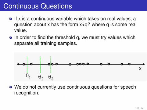
Continuous Questions
If x is a continuous variable which takes on real values, aquestion about x has the form x<q? where q is some realvalue.In order to find the threshold q, we must try values whichseparate all training samples.
We do not currently use continuous questions for speechrecognition.
108 / 141
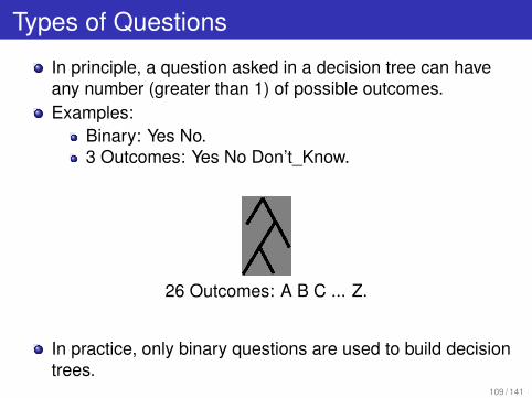
Types of Questions
In principle, a question asked in a decision tree can haveany number (greater than 1) of possible outcomes.Examples:
Binary: Yes No.3 Outcomes: Yes No Don’t_Know.
26 Outcomes: A B C ... Z.
In practice, only binary questions are used to build decisiontrees.
109 / 141
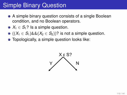
Simple Binary Question
A simple binary question consists of a single Booleancondition, and no Boolean operators.X1 ∈ S1? Is a simple question.((X1 ∈ S1)&&(X2 ∈ S2))? is not a simple question.Topologically, a simple question looks like:
110 / 141
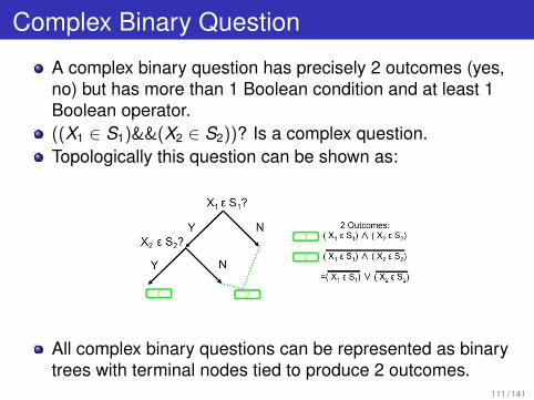
Complex Binary Question
A complex binary question has precisely 2 outcomes (yes,no) but has more than 1 Boolean condition and at least 1Boolean operator.((X1 ∈ S1)&&(X2 ∈ S2))? Is a complex question.Topologically this question can be shown as:
All complex binary questions can be represented as binarytrees with terminal nodes tied to produce 2 outcomes.
111 / 141
Configurations Currently Used
All decision trees currently used in speech recognition use:a pre-determined setof simple,binary questions.on discrete variables.
112 / 141

Tree Construction Overview
Let x1 . . . xn denote n discrete variables whose values maybe asked about. Let Qij denote the j th pre-determinedquestion for xi .Starting at the root, try splitting each node into 2 sub-nodes:
1 For each xi evaluate questions Qi1, Qi2, . . . and let Q′i
denote the best.2 Find the best pair xi , Q′
i and denote it x ′, Q′
3 If Q′ is not sufficiently helpful, make the current node aleaf.
4 Otherwise, split the current node into 2 new sub-nodesaccording to the answer of question Q′ on variable x ′.
Stop when all nodes are either too small to split further orhave been marked as leaves.
113 / 141
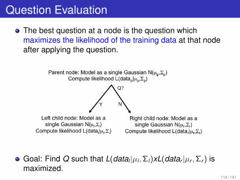
Question Evaluation
The best question at a node is the question whichmaximizes the likelihood of the training data at that nodeafter applying the question.
Goal: Find Q such that L(datal |µl , Σl)xL(datar |µr , Σr ) ismaximized.
114 / 141
Question Evaluation, cont’d
Let feature x have a set of M possible outcomes.Let x1, x2, . . . , xN be the data samples for feature xLet each of the M outcomes occur ci(i = 1, 2, . . . , M) timesin the overall sampleLet Q be a question which partitions this sample into leftand right sub-samples of size nl and nr , respectively.Let c l
i , cri denote the frequency of the i th outcome in the left
and right sub-samples.The best question Q for feature x is defined to be the onewhich maximizes the conditional (log) likelihood of thecombined sub-samples.
115 / 141
log likelihood computation
The log likelihood of the data, given that we ask question Q,is:
log L(x1, . . . , xn|Q) =N∑
i=1
c li log pl
i +N∑
i=1
cri log pr
i
The above assumes we know the "true" probabilities pli , pr
i
116 / 141
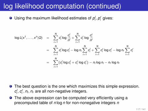
log likelihood computation (continued)
Using the maximum likelihood estimates of pli , pr
i gives:
log L(x1, . . . , xn|Q) =NX
i=1
c li log
c li
nl+
NXi=1
cri log
cri
nr
=NX
i=1
c li log c l
i − log nl
NXi=1
c li +
NXi=1
cri log cr
i − log nr
NXi=1
cri
=NX
i=1
{c li log c l
i + cri log cr
i } − nl log nl − nr log nr
The best question is the one which maximizes this simple expression.c l
i , cri , nl , nr are all non-negative integers.
The above expression can be computed very efficiently using aprecomputed table of n log n for non-nonegative integers n
117 / 141
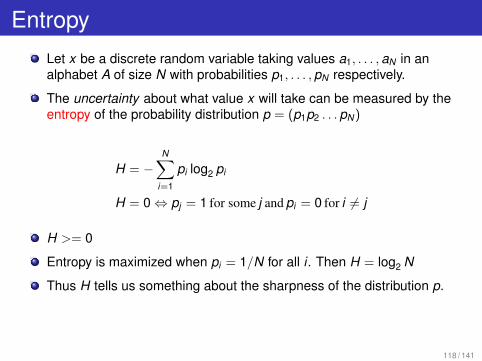
Entropy
Let x be a discrete random variable taking values a1, . . . , aN in analphabet A of size N with probabilities p1, . . . , pN respectively.
The uncertainty about what value x will take can be measured by theentropy of the probability distribution p = (p1p2 . . . pN)
H = −N∑
i=1
pi log2 pi
H = 0 ⇔ pj = 1 for some j and pi = 0 for i 6= j
H >= 0
Entropy is maximized when pi = 1/N for all i . Then H = log2 N
Thus H tells us something about the sharpness of the distribution p.
118 / 141

What does entropy look like for a binaryvariable?
119 / 141
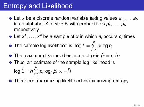
Entropy and Likelihood
Let x be a discrete random variable taking values a1, . . . aN
in an alphabet A of size N with probabilities p1, . . . , pN
respectively.Let x1, . . . , xn be a sample of x in which ai occurs ci times
The sample log likelihood is: log L =n∑
i=1ci log pi
The maximum likelihood estimate of pi is pi = ci/nThus, an estimate of the sample log likelihood is
log L = nN∑
i=1pi log2 pi ∝ −H
Therefore, maximizing likelihood ⇔ minimizing entropy.
120 / 141
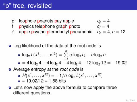
“p” tree, revisited
p loophole peanuts pay apple cp = 4f physics telephone graph photo cf = 4φ apple psycho pterodactyl pneumonia cφ = 4, n = 12
Log likelihood of the data at the root node is
log2 L(x1, . . . , x12) =3∑
i=1ci log2 ci − n log2 n
= 4 log2 4 + 4 log2 4 + 4 log2 4− 12 log2 12 = −19.02Average entropy at the root node is
H(x1, . . . , x12) = −1/n log2 L(x1, . . . , x12)= 19.02/12 = 1.58 bits
Let’s now apply the above formula to compare threedifferent questions.
121 / 141

“p” tree revisited: Question A
122 / 141
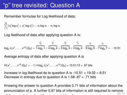
“p” tree revisited: Question A
Remember formulae for Log likelihood of data:
NPi=1
{c li log c l
i + cri log cr
i } − nl log nl − nr log nr
Log likelihood of data after applying question A is:
log2 L(x1, . . . , x12|QA) =
clpz }| {
1 log2 1 +
clfz }| {
4 log2 4 +
crpz }| {
3 log2 3 +
crφz }| {
4 log2 4−
nlz }| {5 log2 5−
nrz }| {7 log2 7 = −10.51
Average entropy of data after applying question A is
H(x1, . . . , x12|QA) = −1/n log2 L(x1, . . . , x12|QA) = 10.51/12 = .87 bits
Increase in log likelihood do to question A is -10.51 + 19.02 = 8.51Decrease in entropy due to question A is 1.58-.87 = .71 bits
Knowing the answer to question A provides 0.71 bits of information about thepronunciation of p. A further 0.87 bits of information is still required to removeall the uncertainty about the pronunciation of p.
123 / 141
“p” tree revisited: Question B
124 / 141
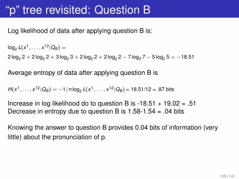
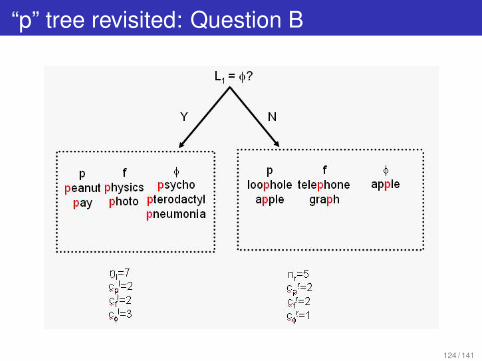
“p” tree revisited: Question B
Log likelihood of data after applying question B is:
log2 L(x1, . . . , x12|QB) =
2 log2 2 + 2 log2 2 + 3 log2 3 + 2 log2 2 + 2 log2 2 − 7 log2 7 − 5 log2 5 = −18.51
Average entropy of data after applying question B is
H(x1, . . . , x12|QB) = −1/n log2 L(x1, . . . , x12|QB) = 18.51/12 = .87 bits
Increase in log likelihood do to question B is -18.51 + 19.02 = .51Decrease in entropy due to question B is 1.58-1.54 = .04 bits
Knowing the answer to question B provides 0.04 bits of information (verylittle) about the pronunciation of p.
125 / 141
“p” tree revisited: Question C
126 / 141

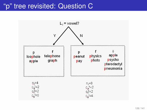
“p” tree revisited: Question C
Log likelihood of data after applying question C is:
log2 L(x1, . . . , x12|QC) =
2 log2 2 + 2 log2 2 + 2 log2 2 + 2 log2 2 + 4 log2 4 − 4 log2 4 − 8 log2 8 = −16.00
Average entropy of data after applying question C is
H(x1, . . . , x12|QC) = −1/n log2 L(x1, . . . , x12|QC) = 16/12 = 1.33 bits
Increase in log likelihood do to question C is -16 + 19.02 = 3.02Decrease in entropy due to question C is 1.58-1.33 = .25 bits
Knowing the answer to question C provides 0.25 bits of information about thepronunciation of p.
127 / 141
Comparison of Questions A, B, C
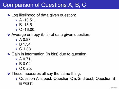
Log likelihood of data given question:A -10.51.B -18.51.C -16.00.
Average entropy (bits) of data given question:A 0.87.B 1.54.C 1.33.
Gain in information (in bits) due to question:A 0.71.B 0.04.C 0.25.
These measures all say the same thing:Question A is best. Question C is 2nd best. Question Bis worst.
128 / 141
Using Decision Trees to Model ContextDependence in HMMs
Remember that the pronunciation of a phone depends onits context.Enumeration of all triphones is one option but has problemsIdea is to use decision trees to find set of equivalenceclasses
129 / 141

Using Decision Trees to Model ContextDependence in HMMs
Align training data (feature vectors) against set ofphonetic-based HMMsFor each feature vector, tag it with ID of current phone andthe phones to left and right.For each phone, create a decision tree by asking questionsabout the phones on left and right to maximize likelihood ofdata.Leaves of tree represent context dependent models for thatphone.During training and recognition, you know the phone and itscontext so no problem in identifying the context-dependentmodels on the fly.
130 / 141
New Problem: dealing with real-valued data
We grow the tree so as to maximize the likelihood of thetraining data (as always), but now the training data arereal-valued vectors.Can’t use the multinomial distribution we used for thespelling-to-sound example,instead, estimate the likelihood of the acoustic vectorsduring tree construction using a diagonal Gaussian model.
131 / 141
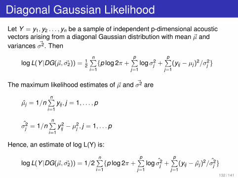
Diagonal Gaussian Likelihood
Let Y = y1, y2 . . . , yn be a sample of independent p-dimensional acousticvectors arising from a diagonal Gaussian distribution with mean ~µ andvariances ~σ2. Then
log L(Y |DG(~µ, ~σ2)) = 12
n∑i=1{p log 2π +
p∑j=1
log σ2j +
p∑j=1
(yij − µj)2/σ2
j }
The maximum likelihood estimates of ~µ and ~σ2 are
µj = 1/nn∑
i=1yij , j = 1, . . . , p
σ2j = 1/n
n∑i=1
y2ij − µ2
j , j = 1, . . . p
Hence, an estimate of log L(Y) is:
log L(Y |DG(~µ, ~σ2)) = 1/2n∑
i=1{p log 2π +
p∑j=1
log σ2j +
p∑j=1
(yij − µj)2/σ2
j }
132 / 141
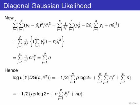
Diagonal Gaussian Likelihood
Nown∑
i=1
p∑j=1
(yij − µj)2/σj
2 =p∑
j=1
1σj
2
n∑i=1
(y2ij − 2µj
n∑i=1
yij + nµj2)
=p∑
j=1
1σj
2
{(
n∑i=1
y2ij )− nµj
2}
=p∑
j=1
1σj
2 nσ2j =
p∑j=1
n
Hence
log L(Y |DG(µ, σ2)) = −1/2{n∑
i=1p log 2π +
n∑i=1
p∑j=1
σj2 +
p∑j=1
n}
= −1/2{np log 2π + np∑
j=1σj
2 + np}
133 / 141
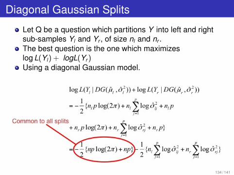
Diagonal Gaussian Splits
Let Q be a question which partitions Y into left and rightsub-samples Yl and Yr , of size nl and nr .The best question is the one which maximizeslog L(Yl) + logL(Yr )Using a diagonal Gaussian model.
134 / 141
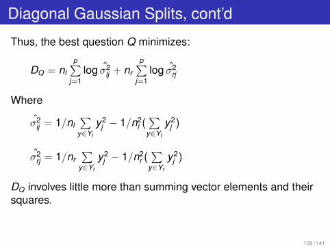
Diagonal Gaussian Splits, cont’d
Thus, the best question Q minimizes:
DQ = nl
p∑j=1
log σ2lj + nr
p∑j=1
log σ2rj
Where
σ2lj = 1/nl
∑y∈Yl
y2j − 1/n2
l (∑
y∈Yl
y2j )
σ2rj = 1/nr
∑y∈Yr
y2j − 1/n2
r (∑
y∈Yr
y2j )
DQ involves little more than summing vector elements and theirsquares.
135 / 141
How Big a Tree?
CART suggests cross-validation.Measure performance on a held-out data set.Choose the tree size that maximizes the likelihood ofthe held-out data.
In practice, simple heuristics seem to work well.A decision tree is fully grown when no terminal node can besplit.Reasons for not splitting a node include:
Insufficient data for accurate question evaluation.Best question was not very helpful / did not improve thelikelihood significantly.Cannot cope with any more nodes due to CPU/memorylimitations.
136 / 141

Recap
Given a word sequence, we can construct thecorresponding Markov model by:
Re-writing word string as a sequence of phonemes.Concatenating phonetic models.Using the appropriate tree for each phone to determinewhich allophone (leaf) is to be used in that context.
In actuality, we make models for the HMM arcs themselvesFollow same process as with phones - align dataagainst the arcsTag each feature vector with its arc id and phoneticcontextCreate decision tree for each arc.
137 / 141
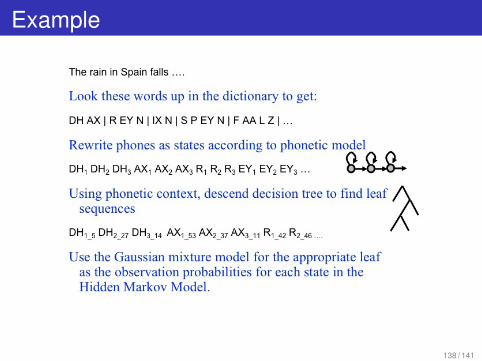
Example
138 / 141
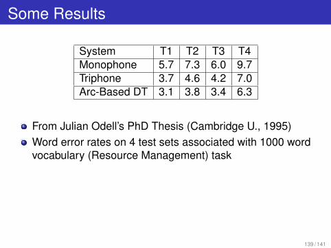
Some Results
System T1 T2 T3 T4Monophone 5.7 7.3 6.0 9.7Triphone 3.7 4.6 4.2 7.0Arc-Based DT 3.1 3.8 3.4 6.3
From Julian Odell’s PhD Thesis (Cambridge U., 1995)Word error rates on 4 test sets associated with 1000 wordvocabulary (Resource Management) task
139 / 141
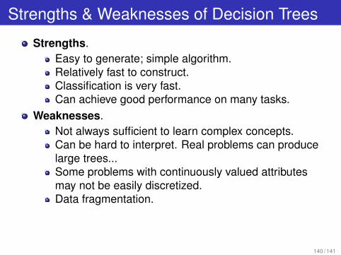
Strengths & Weaknesses of Decision Trees
Strengths.Easy to generate; simple algorithm.Relatively fast to construct.Classification is very fast.Can achieve good performance on many tasks.
Weaknesses.Not always sufficient to learn complex concepts.Can be hard to interpret. Real problems can producelarge trees...Some problems with continuously valued attributesmay not be easily discretized.Data fragmentation.
140 / 141
Course Feedback
Was this lecture mostly clear or unclear?What was the muddiest topic?Other feedback (pace, content, atmosphere, etc.).
141 / 141
Top Related