ISOTOPES AND LAND PLANT ECOLOGY

C3 vs. C4 vs. CAM

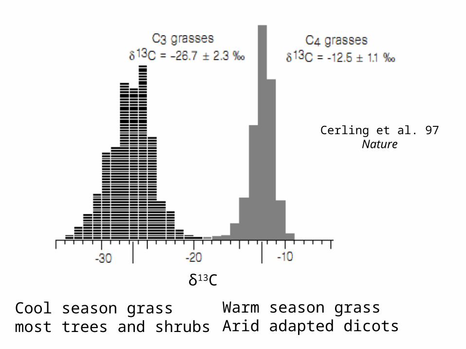
Cool season grassmost trees and shrubs

Warm season grassArid adapted dicots

Cerling et al. 97Nature

δ13C

εp = δa - δf = εt + (Ci/Ca)(εf-εt)

When Ci ≈ Ca (low rate of photosynthesis, open stomata), then εp ≈ εf. Large fractionation, low plant δ13C values.

When Ci << Ca (high rate of photosynthesis, closed stomata), then εp ≈ εt. Small fractionation, high plant δ13C values.

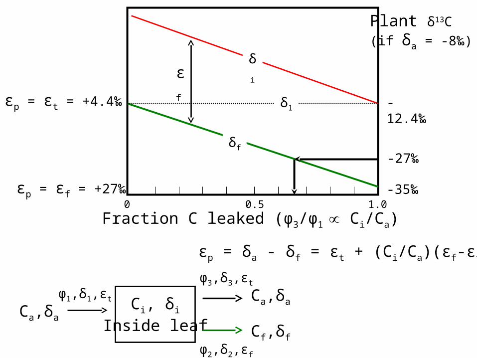
Ci, δi

Inside leafCa,δa

Ca,δa

Cf,δf

φ1,δ1,εt

φ3,δ3,εt

φ2,δ2,εf

-12.4‰

-35‰

-27‰

Plant δ13C

(if δa = -8‰)

εp = εt = +4.4‰

εp = εf = +27‰

εf

0 0.5 1.0

Fraction C leaked (φ3/φ1 C∝ i/Ca)

δi

δf

δ1

εp = δa - δf = εt + (Ci/Ca)(εf-εt)

(Relative to preceding slide, note that the Y axis is reversed, so that εp increases up the scale)

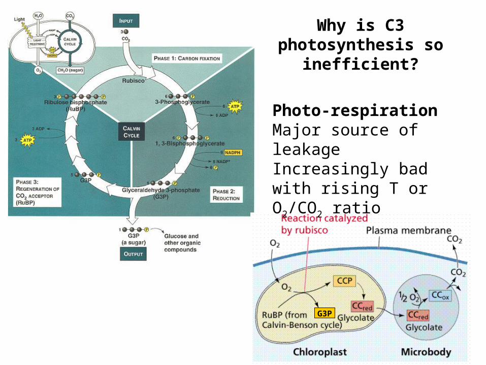
G3P

Photo-respirationMajor source of leakageIncreasingly bad with rising T or O2/CO2 ratio

Why is C3 photosynthesis so inefficient?

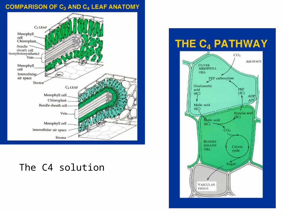
The C4 solution

CO2 a

δa

φ1,δ1

φ3,δ3

δi CO2 i

(aq)

HCO3

Δi-εd/b

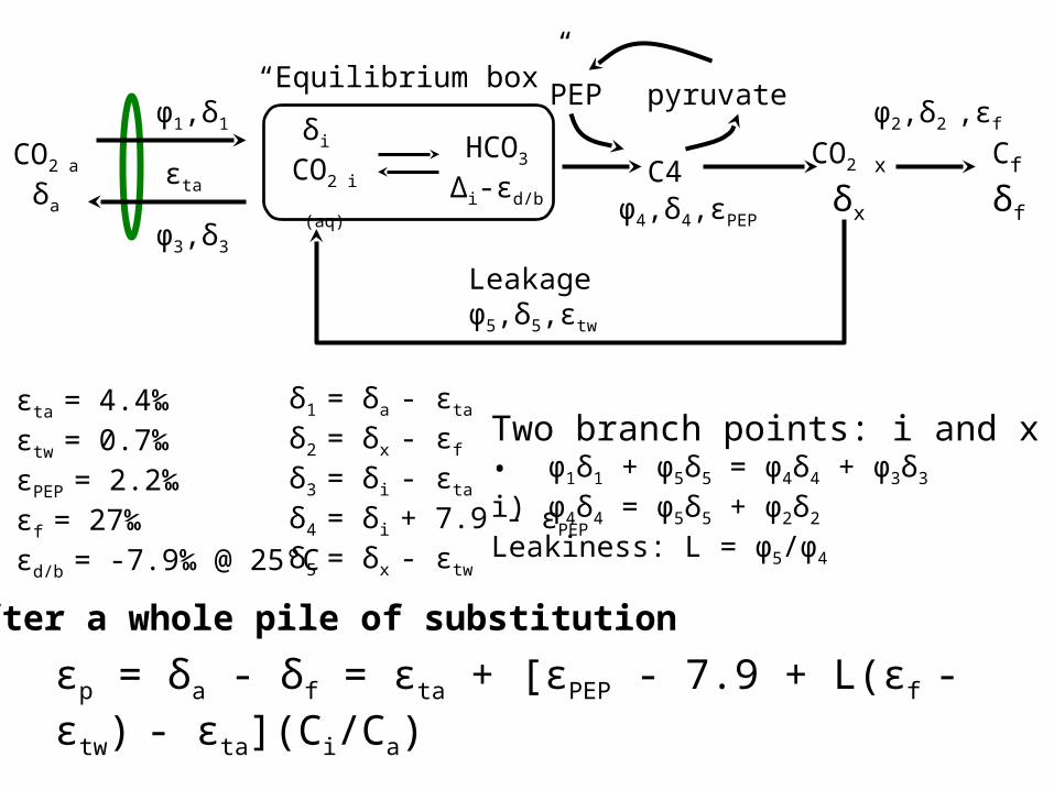
“Equilibrium box”

C4

PEP pyruvate

CO2 xδx

Cf

δf

φ2,δ2 ,εf

φ4,δ4,εPEP

Leakageφ5,δ5,εtw

εta

εta = 4.4‰εtw = 0.7‰εPEP = 2.2‰εf = 27‰εd/b = -7.9‰ @ 25°C

δ1 = δa - εta δ2 = δx - εf

δ3 = δi - εta

δ4 = δi + 7.9 - εPEP

δ5 = δx - εtw

Two branch points: i and x• φ1δ1 + φ5δ5 = φ4δ4 + φ3δ3

i) φ4δ4 = φ5δ5 + φ2δ2

Leakiness: L = φ5/φ4

After a whole pile of substitution

εp = δa - δf = εta + [εPEP - 7.9 + L(εf - εtw) - εta](Ci/Ca)

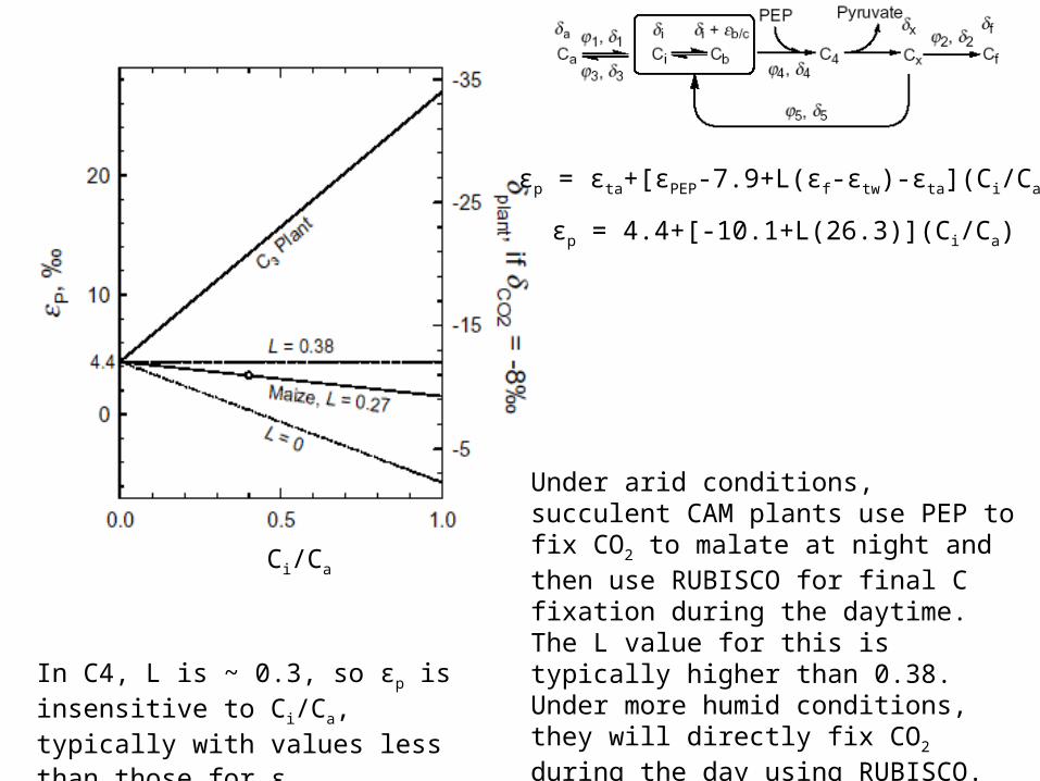
Ci/Ca

In C4, L is ~ 0.3, so εp is insensitive to Ci/Ca, typically with values less than

those for εta.

εp = εta+[εPEP-7.9+L(εf-εtw)-εta](Ci/Ca)

Under arid conditions, succulent CAM plants use PEP to fix CO2 to malate at night and then use RUBISCO for final C fixation during the daytime. The L value for this is typically higher than 0.38. Under more humid conditions, they will directly fix CO2 during the day using RUBISCO. As a consequence, they have higher, and more variable, εp values.

εp = 4.4+[-10.1+L(26.3)](Ci/Ca)

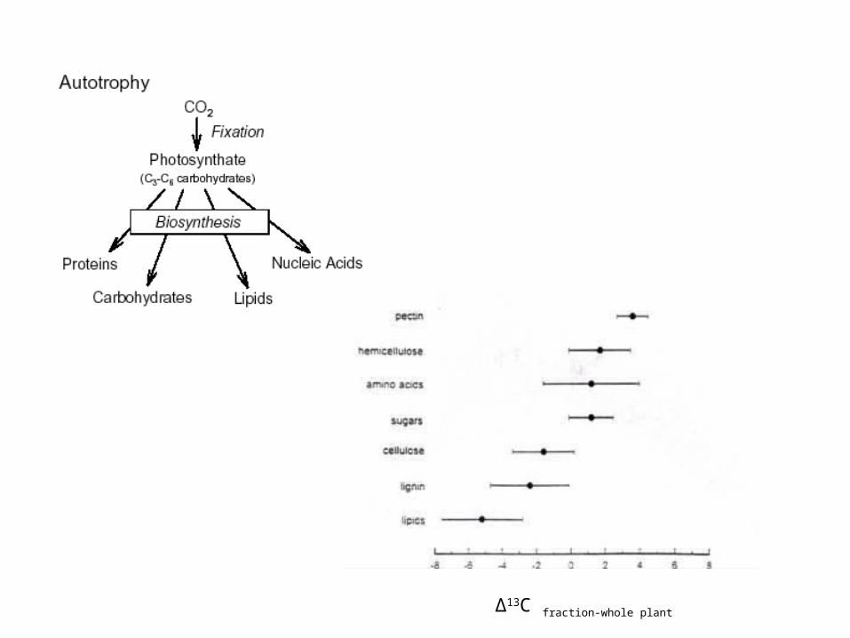
Δ13C fraction-whole plant

Environmental Controls on plant δ13C values

Temperature, water stress, light level, height in the canopy, E.T.C . . .

δ13C varies with environment within C3 plants

C3 plants

QuickTime™ and aTIFF (Uncompressed) decompressor

are needed to see this picture.

soil water

QuickTime™ and aTIFF (Uncompressed) decompressor

are needed to see this picture.

drought

normal

εp = εt + (Ci/Ca)(εf-εt)

When its dry, plants keep theirstomata shut. Drive down Ci/Ca.

C3

drywet

Much less variability in C4, except for different C4 pathways.

NADP C4 > NAD or PCK C4

Water Use Efficiency (WUE) = Assimilation rate/transpiration rate

WUE is negatively correlated with Ci/Ca and therefore negatively correlated with εp or Δ, for a constant v (vapor pressure difference)

Evergreen higher WUE than decid.

A/E = (Ca-Ci)/1.6v = Ca (( 1-Ci )/Ca) /1.6v

QuickTime™ and aTIFF (Uncompressed) decompressor

are needed to see this picture.

salty fresh

Salinity stress = Water stress

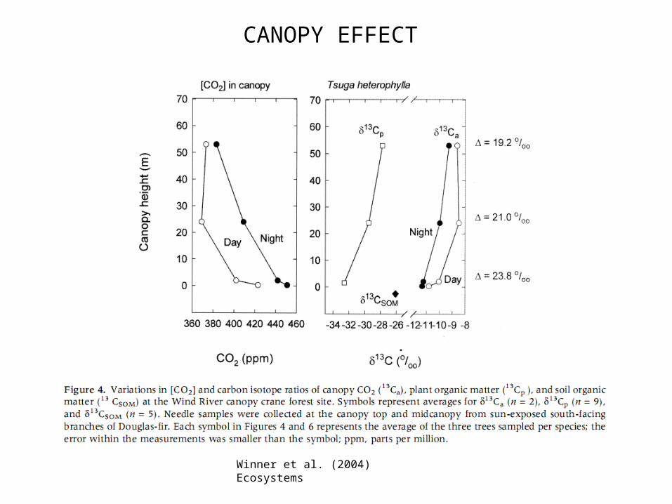
CANOPY EFFECT

Winner et al. (2004) Ecosystems

QuickTime™ and aTIFF (Uncompressed) decompressor

are needed to see this picture.

Diurnal variation

Light matters too

Buchman et al. (1997) Oecologia

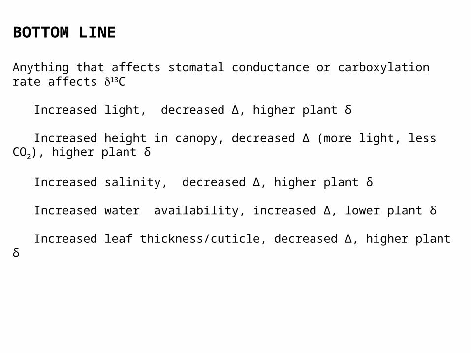
BOTTOM LINE

Anything that affects stomatal conductance or carboxylation rate affects 13C

Increased light, decreased Δ, higher plant δ

Increased height in canopy, decreased Δ (more light, less CO2), higher plant δ

Increased salinity, decreased Δ, higher plant δ

Increased water availability, increased Δ, lower plant δ

Increased leaf thickness/cuticle, decreased Δ, higher plant δ

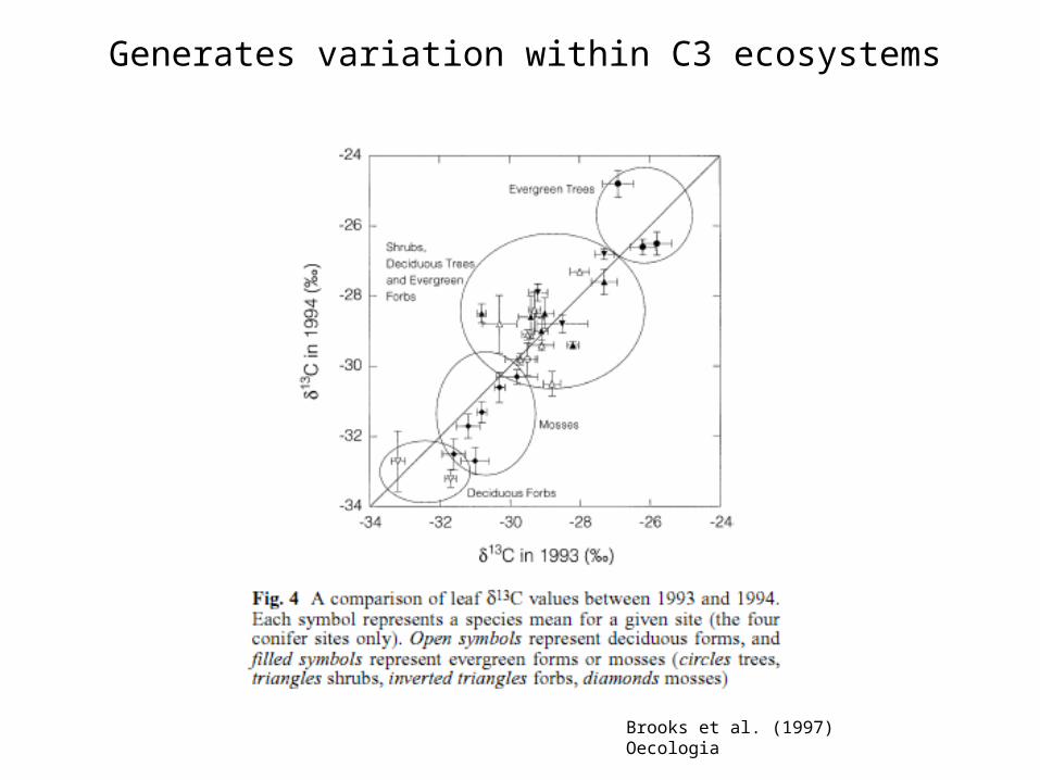
Generates variation within C3 ecosystems

Brooks et al. (1997) Oecologia

QuickTime™ and a decompressor

are needed to see this picture.

Heaton (1999) Journal of Archaeological Science

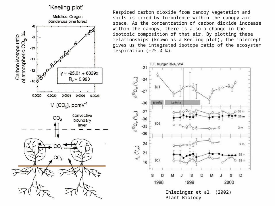
Ehleringer et al. (2002) Plant Biology

Respired carbon dioxide from canopy vegetation and soils is mixed by turbulence within the canopy air space. As the concentration of carbon dioxide increase within the canopy, there is also a change in the isotopic composition of that air. By plotting these relationships (known as a Keeling plot), the intercept gives us the integrated isotope ratio of the ecosystem respiration (-25.0 ‰).

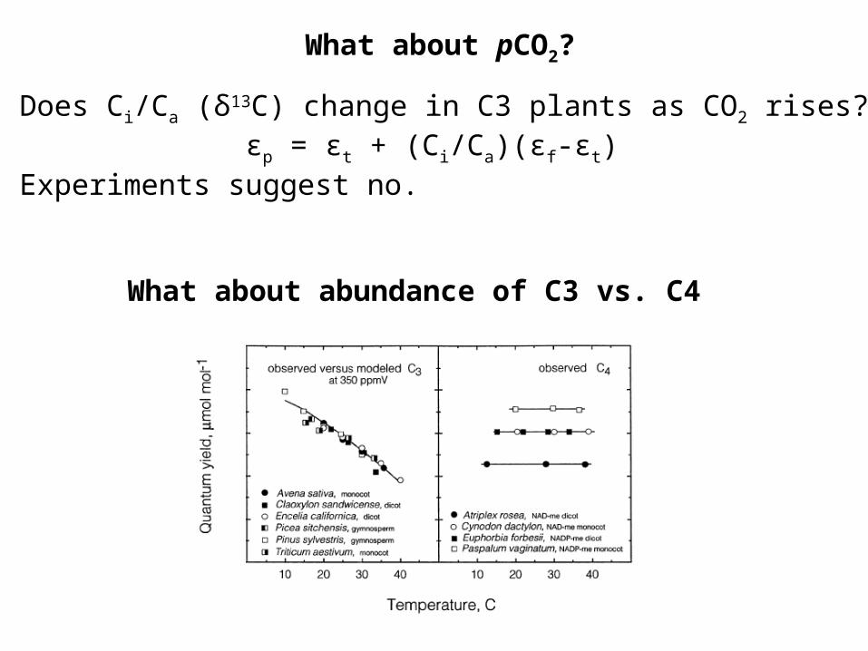
What about pCO2?

Does Ci/Ca (δ13C) change in C3 plants as CO2 rises? εp = εt + (Ci/Ca)(εf-εt)Experiments suggest no.

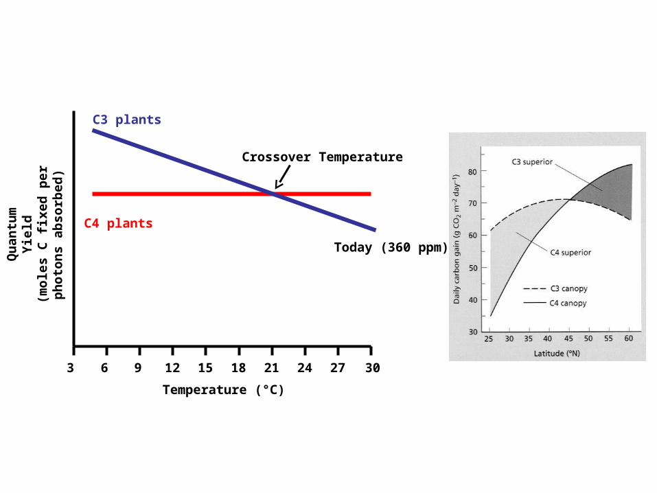
What about abundance of C3 vs. C4

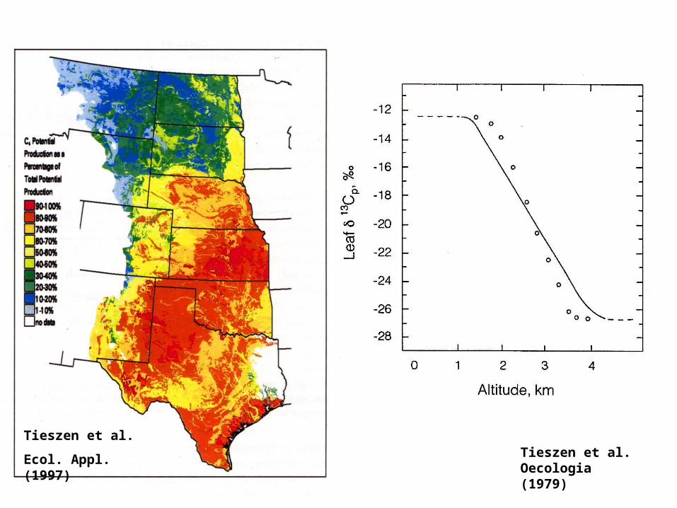
Tieszen et al.

Ecol. Appl. (1997) Tieszen et al. Oecologia (1979)

Qu

antu

mY

ield

(mo

les

C f

ixed

per

ph

oto

ns

abso

rbed

)

Temperature (°C)

3 6 9 12 15 18 21 24 27 30

C4 plants

C3 plants

Crossover Temperature

Today (360 ppm)

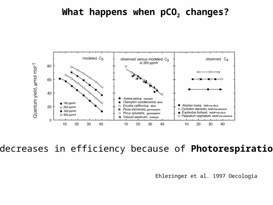
What happens when pCO2 changes?

Ehleringer et al. 1997 Oecologia

C3 decreases in efficiency because of Photorespiration

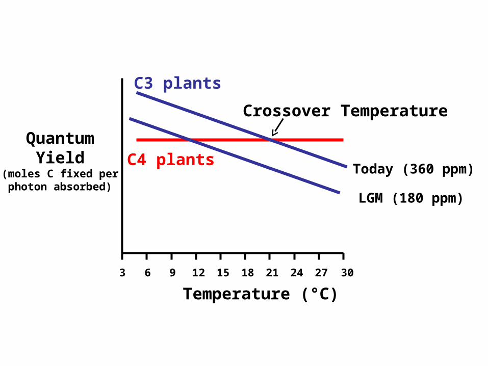
QuantumYield

(moles C fixed perphoton absorbed)

Temperature (°C)

3 6 9 12 15 18 21 24 27 30

C4 plants

C3 plants

Crossover Temperature

Today (360 ppm)

LGM (180 ppm)

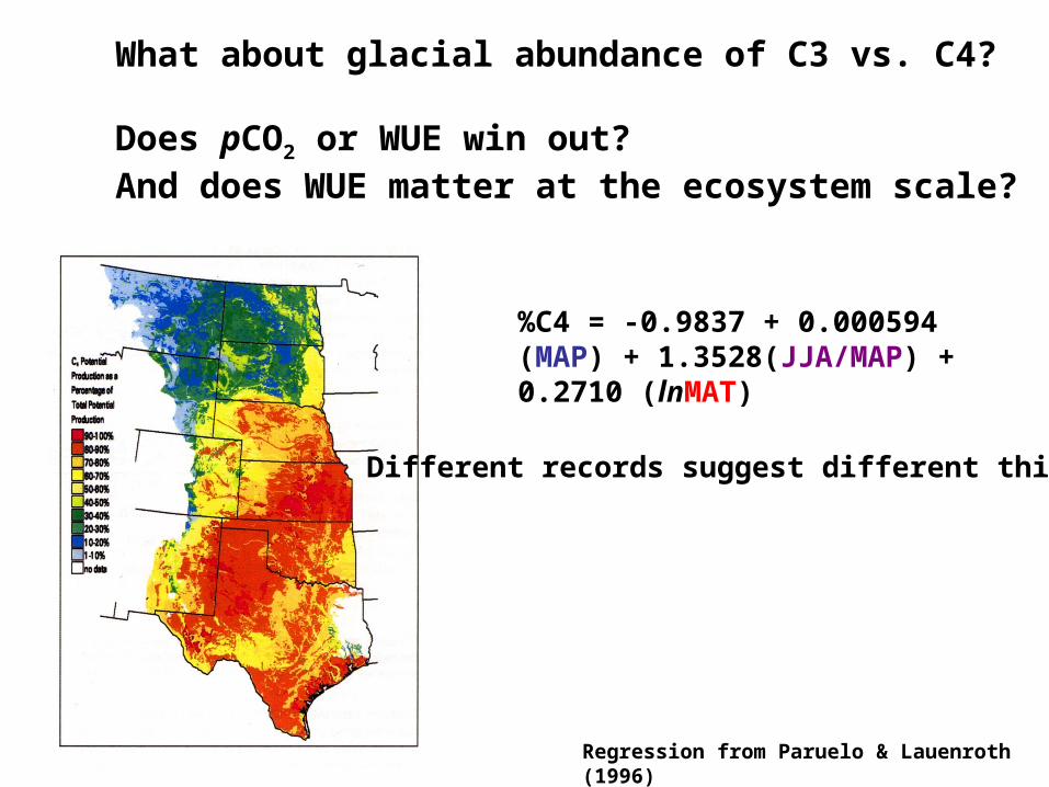
What about glacial abundance of C3 vs. C4?

Does pCO2 or WUE win out?And does WUE matter at the ecosystem scale?

%C4 = -0.9837 + 0.000594 (MAP) + 1.3528(JJA/MAP) + 0.2710 (lnMAT)

Regression from Paruelo & Lauenroth (1996)

Different records suggest different things

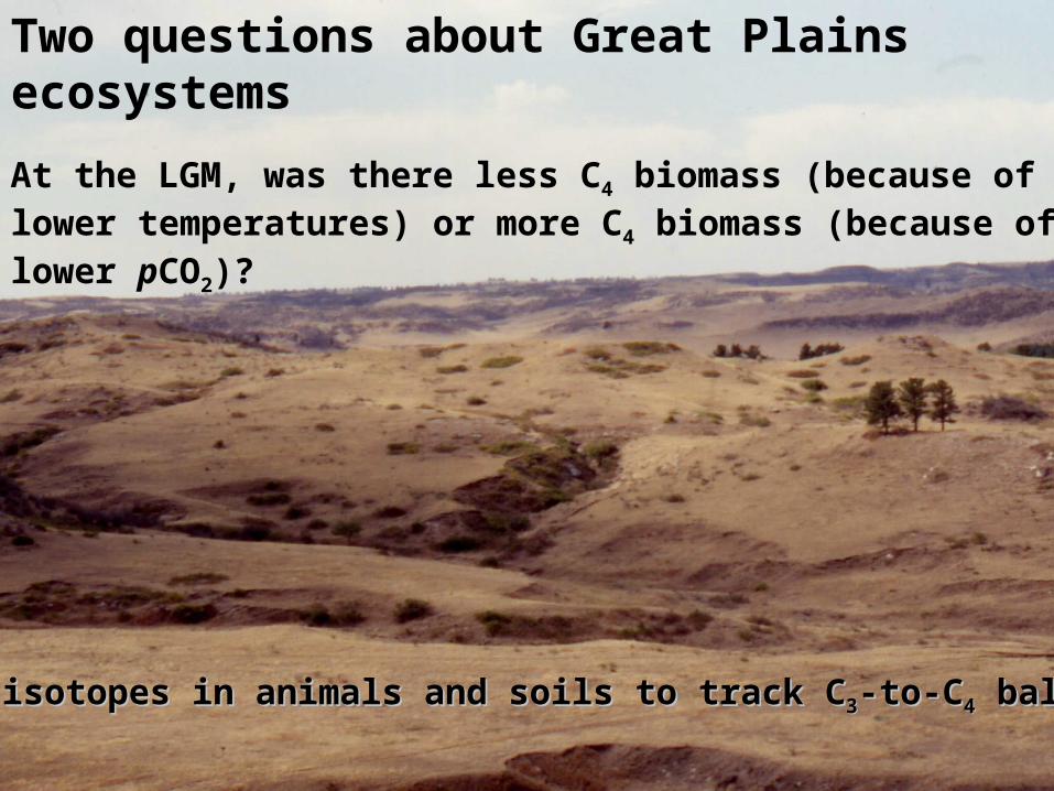
Two questions about Great Plains ecosystems

At the LGM, was there less C4 biomass (because of lower temperatures) or more C4 biomass (because of lower pCO2)?

Use isotopes in animals and soils to track CUse isotopes in animals and soils to track C33-to-C-to-C44 balance balance

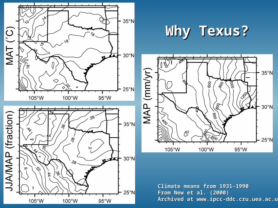
Why Texus?Why Texus?

Climate means from 1931-1990Climate means from 1931-1990From New et al. (2000)From New et al. (2000)Archived at www.ipcc-ddc.cru.uea.ac.ukArchived at www.ipcc-ddc.cru.uea.ac.uk

106°W 104°W 102°W 100°W 98°W 96°W 94°W

26°N

28°N

30°N

32°N

OKLAHOMA

MEXICO

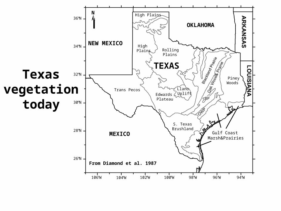
TEXAS

Trans PecosEdwardsPlateau

RollingPlains

S. TexasBrushland

PineyWoods

LlanoUplift

Gulf CoastMarsh&Prairies

BP

34°N

36°N

NEW MEXICO

N

HighPlains

High Plains

From Diamond et al. 1987

Texasvegetation

today

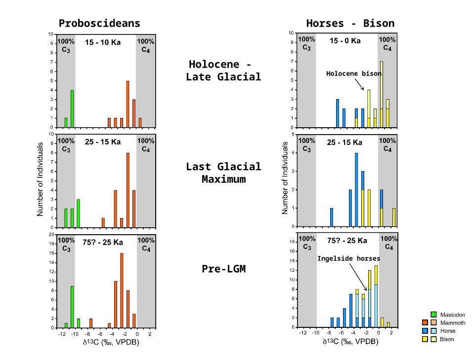
Holocene - Late Glacial

Last GlacialMaximum

Pre-LGM

Proboscideans

Holocene bison

Ingelside horses

Horses - Bison

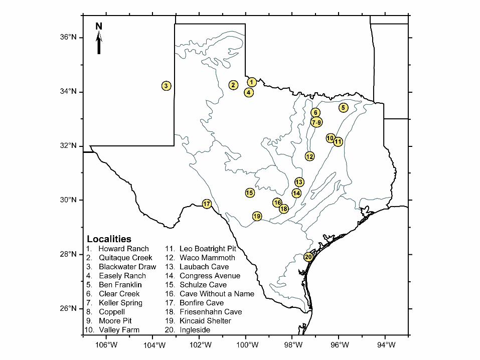
Initial conclusions from isotope studies of Texas mammals

1) No changes in mean δ13C value through time.

1) Bison and mammoths are grazers. They can be used to monitor C3 to C4 balance on Pleistocene grasslands.

2) Mastodons are browsers. Their presence suggests tree cover.

3) Pleistocene horses ate lots of C3 vegetation, even when bison and mammoths had ~100% C4 diets. Horses were mixed feeders.

What's next?Compare %C4 from mammals to values simulated via modeling.

1) Use Quaternary climate model output, and estimate %C4 biomass using the Regression Equation.

2) Use the same climate model output, but estimate %C4 biomass as the percentage of growing season months that are above the appropriate Crossover Temperature.

Holocene0-10 Ka

Post-LGM10-15 Ka

LGM25-15 Ka

%C4 Grass from Regression Model

%C4 plants in grazer dietsMammuthus

Bison

Mammut present

Holocene model driven by modern climate data from New et al. (2000). LGM and Post-LGM models driven by GCM output from Kutzbach et al. (1996)(archived at www.ngdc.noaa.gov/paleo/paleo.html)

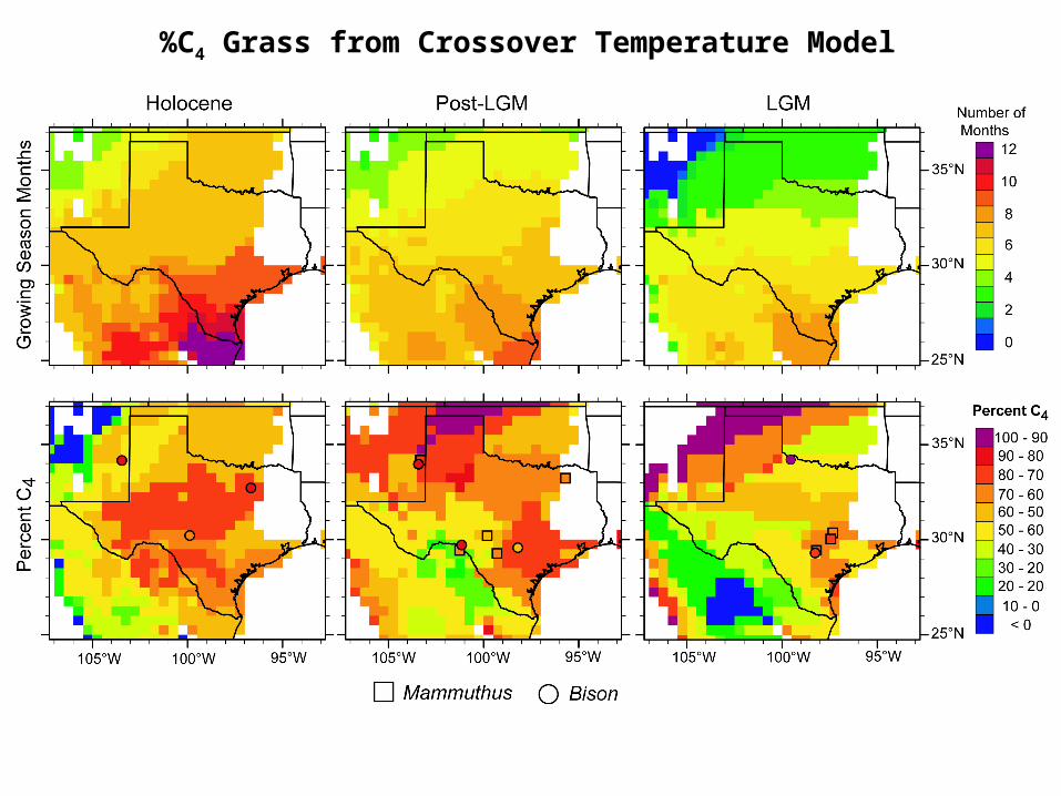
%C4 Grass from Crossover Temperature Model

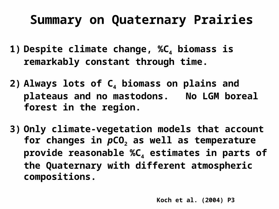
Summary on Quaternary Prairies

1) Despite climate change, %C4 biomass is remarkably constant through time.

2) Always lots of C4 biomass on plains and plateaus and no mastodons. No LGM boreal forest in the region.

3) Only climate-vegetation models that account for changes in pCO2 as well as temperature provide reasonable %C4 estimates in parts of the Quaternary with different atmospheric compositions.

Koch et al. (2004) P3