Inverse Problems:From Regularization to Bayesian Inference

An Overview onPrior Modeling and Bayesian Computation

Application to Computed Tomography

Ali Mohammad-Djafari

Groupe Problemes InversesLaboratoire des Signaux et Systemes

UMR 8506 CNRS - SUPELEC - Univ Paris Sud 11Supelec, Plateau de Moulon, 91192 Gif-sur-Yvette, FRANCE.

djafari@lss.supelec.frhttp://djafari.free.fr

http://www.lss.supelec.fr

Applied Math Colloquium, UCLA, USA, July 17, 2009Organizer: Stanley Osher

1 / 42

Content Image reconstruction in Computed Tomography :

An ill posed invers problem Two main steps in Bayesian approach :

Prior modeling and Bayesian computation Prior models for images :

Separable Gaussian, GG, ... Gauss-Markov, General one layer Markovian models Hierarchical Markovian models with hidden variables

(contours and regions) Gauss-Markov-Potts

Bayesian computation MCMC Variational and Mean Field approximations (VBA, MFA)

Application : Computed Tomography in NDT Conclusions and Work in Progress Questions and Discussion

2 / 42

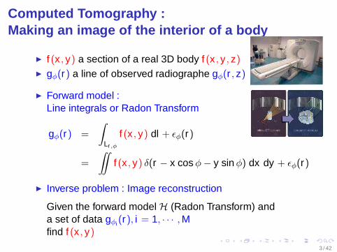
Computed Tomography :Making an image of the interior of a body

f (x , y) a section of a real 3D body f (x , y , z)

gφ(r) a line of observed radiographe gφ(r , z)

Forward model :Line integrals or Radon Transform

gφ(r) =

∫

Lr ,φ

f (x , y) dl + ǫφ(r)

=

∫∫f (x , y) δ(r − x cos φ − y sin φ) dx dy + ǫφ(r)

Inverse problem : Image reconstruction

Given the forward model H (Radon Transform) anda set of data gφi (r), i = 1, · · · , Mfind f (x , y)

3 / 42

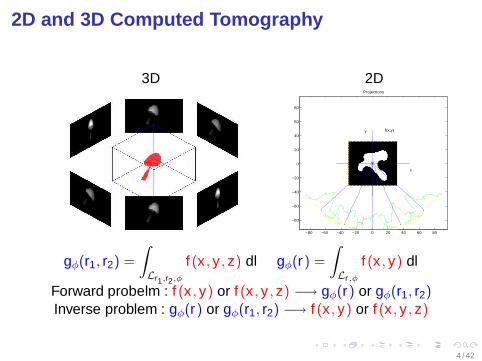
2D and 3D Computed Tomography

3D 2D

−80 −60 −40 −20 0 20 40 60 80

−80

−60

−40

−20

0

20

40

60

80

f(x,y)

x

y

Projections

gφ(r1, r2) =

∫

Lr1,r2,φ

f (x , y , z) dl gφ(r) =

∫

Lr ,φ

f (x , y) dl

Forward probelm : f (x , y) or f (x , y , z) −→ gφ(r) or gφ(r1, r2)Inverse problem : gφ(r) or gφ(r1, r2) −→ f (x , y) or f (x , y , z)

4 / 42

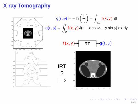
X ray Tomography

f(x,y)

x

y

−150 −100 −50 0 50 100 150

−150

−100

−50

0

50

100

150

g(r , φ) = − ln(

II0

)=

∫

Lr,φ

f (x , y) dl

g(r , φ) =

∫∫

Df (x , y) δ(r − x cos φ − y sin φ) dx dy

f (x , y)- RT -g(r , φ)

phi

r

p(r,phi)

0

45

90

135

180

225

270

315

IRT?

=⇒−60 −40 −20 0 20 40 60

−60

−40

−20

0

20

40

60

5 / 42

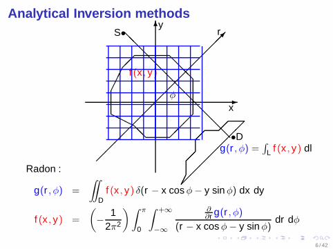
Analytical Inversion methods

f (x , y)

-x

6y

@@@

@@

HHH

r

φ

•Dg(r , φ) =

∫L f (x , y) dl

S•

@@

@@

@@

@@

@@

@@

Radon :

g(r , φ) =

∫∫

Df (x , y) δ(r − x cos φ − y sin φ) dx dy

f (x , y) =

(−

12π2

)∫ π

0

∫ +∞

−∞

∂∂r g(r , φ)

(r − x cos φ − y sin φ)dr dφ

6 / 42

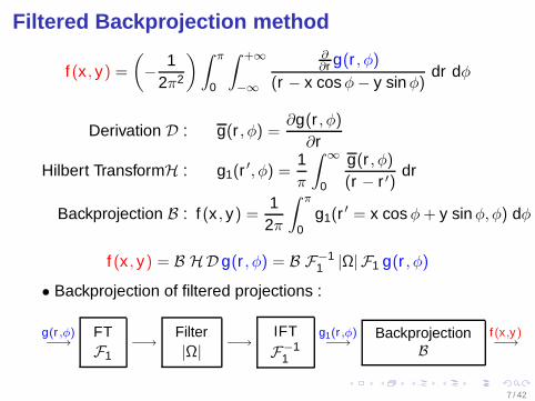
Filtered Backprojection method

f (x , y) =

(−

12π2

) ∫ π

0

∫ +∞

−∞

∂∂r g(r , φ)

(r − x cos φ − y sin φ)dr dφ

Derivation D : g(r , φ) =∂g(r , φ)

∂r

Hilbert TransformH : g1(r′, φ) =

1π

∫ ∞

0

g(r , φ)

(r − r ′)dr

Backprojection B : f (x , y) =1

2π

∫ π

0g1(r

′ = x cos φ + y sin φ, φ) dφ

f (x , y) = B HD g(r , φ) = B F−11 |Ω| F1 g(r , φ)

• Backprojection of filtered projections :

g(r ,φ)−→

FTF1

−→Filter|Ω|

−→IFTF−1

1

g1(r ,φ)−→

BackprojectionB

f (x,y)−→

7 / 42

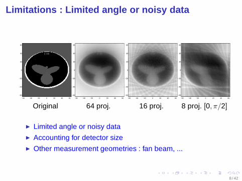
Limitations : Limited angle or noisy data

−60 −40 −20 0 20 40 60

−60

−40

−20

0

20

40

60

−60 −40 −20 0 20 40 60

−60

−40

−20

0

20

40

60

−60 −40 −20 0 20 40 60

−60

−40

−20

0

20

40

60

−60 −40 −20 0 20 40 60

−60

−40

−20

0

20

40

60

Original 64 proj. 16 proj. 8 proj. [0, π/2]

Limited angle or noisy data Accounting for detector size Other measurement geometries : fan beam, ...

8 / 42

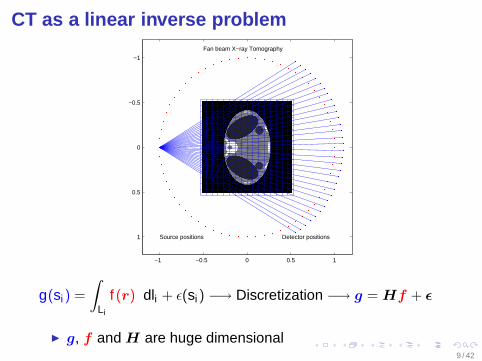
CT as a linear inverse problem

Source positions Detector positions

Fan beam X−ray Tomography

−1 −0.5 0 0.5 1

−1

−0.5

0

0.5

1

g(si) =

∫

Li

f (r) dli + ǫ(si) −→ Discretization −→ g = Hf + ǫ

g, f and H are huge dimensional9 / 42

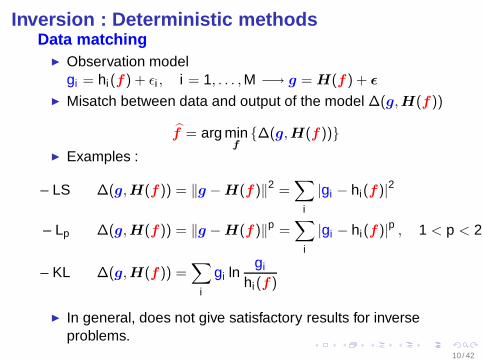
Inversion : Deterministic methodsData matching

Observation modelgi = hi(f) + ǫi , i = 1, . . . , M −→ g = H(f ) + ǫ

Misatch between data and output of the model ∆(g,H(f ))

f = arg minf

∆(g,H(f ))

Examples :

– LS ∆(g,H(f )) = ‖g − H(f )‖2 =∑

i

|gi − hi(f)|2

– Lp ∆(g,H(f )) = ‖g − H(f )‖p =∑

i

|gi − hi(f)|p , 1 < p < 2

– KL ∆(g,H(f )) =∑

i

gi lngi

hi(f)

In general, does not give satisfactory results for inverseproblems.

10 / 42

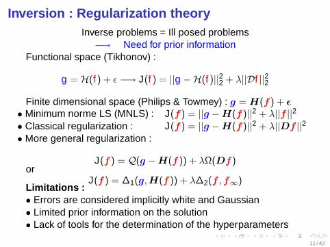
Inversion : Regularization theoryInverse problems = Ill posed problems

−→ Need for prior informationFunctional space (Tikhonov) :

g = H(f ) + ǫ −→ J(f ) = ||g −H(f )||22 + λ||Df ||22

Finite dimensional space (Philips & Towmey) : g = H(f) + ǫ

• Minimum norme LS (MNLS) : J(f ) = ||g − H(f )||2 + λ||f ||2

• Classical regularization : J(f ) = ||g − H(f )||2 + λ||Df ||2

• More general regularization :

J(f ) = Q(g − H(f )) + λΩ(Df)or

J(f) = ∆1(g,H(f )) + λ∆2(f ,f∞)Limitations :• Errors are considered implicitly white and Gaussian• Limited prior information on the solution• Lack of tools for the determination of the hyperparameters

11 / 42

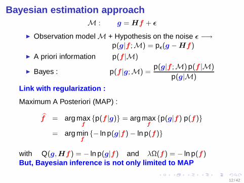
Bayesian estimation approachM : g = Hf + ǫ

Observation model M + Hypothesis on the noise ǫ −→p(g|f ;M) = pǫ(g − Hf)

A priori information p(f |M)

Bayes : p(f |g;M) =p(g|f ;M) p(f |M)

p(g|M)

Link with regularization :

Maximum A Posteriori (MAP) :

f = arg maxf

p(f |g) = arg maxf

p(g|f) p(f)

= arg minf

− ln p(g|f) − ln p(f)

with Q(g,Hf ) = − ln p(g|f) and λΩ(f) = − ln p(f)But, Bayesian inference is not only limited to MAP

12 / 42

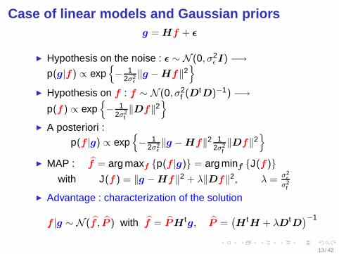
Case of linear models and Gaussian priorsg = Hf + ǫ

Hypothesis on the noise : ǫ ∼ N (0, σ2ǫ I) −→

p(g|f) ∝ exp− 1

2σ2ǫ‖g − Hf‖2

Hypothesis on f : f ∼ N (0, σ2f (DtD)−1) −→

p(f) ∝ exp− 1

2σ2f‖Df‖2

A posteriori :

p(f |g) ∝ exp− 1

2σ2ǫ‖g − Hf‖2 1

2σ2f‖Df‖2

MAP : f = arg maxf p(f |g) = arg minf J(f )

with J(f ) = ‖g − Hf‖2 + λ‖Df‖2, λ = σ2ǫ

σ2f

Advantage : characterization of the solution

f |g ∼ N (f , P ) with f = PH tg, P =(H tH + λDtD

)−1

13 / 42

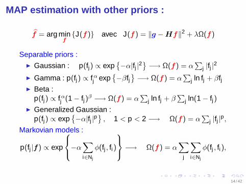
MAP estimation with other priors :

f = arg minf

J(f ) avec J(f ) = ‖g − Hf‖2 + λΩ(f)

Separable priors : Gaussian : p(fj) ∝ exp

−α|fj |2

−→ Ω(f) = α

∑j |fj |

2

Gamma : p(fj) ∝ f αj exp

−βfj

−→ Ω(f) = α

∑j ln fj + βfj

Beta :p(fj) ∝ f α

j (1 − fj)β −→ Ω(f) = α∑

j ln fj + β∑

j ln(1 − fj) Generalized Gaussian :

p(fj) ∝ exp−α|fj |p

, 1 < p < 2 −→ Ω(f) = α

∑j |fj |

p,

Markovian models :

p(fj |f) ∝ exp

−α∑

i∈Nj

φ(fj , fi )

−→ Ω(f) = α∑

j

∑

i∈Nj

φ(fj , fi),

14 / 42

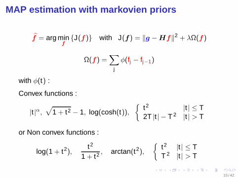
MAP estimation with markovien priors

f = arg minf

J(f ) with J(f) = ‖g − Hf‖2 + λΩ(f)

Ω(f) =∑

j

φ(fj − fj−1)

with φ(t) :

Convex functions :

|t |α,√

1 + t2 − 1, log(cosh(t)),

t2 |t | ≤ T2T |t | − T 2 |t | > T

or Non convex functions :

log(1 + t2),t2

1 + t2 , arctan(t2),

t2 |t | ≤ TT 2 |t | > T

15 / 42

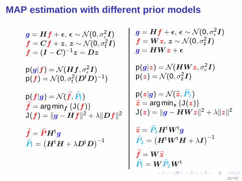
MAP estimation with different prior models

g = Hf + ǫ, ǫ ∼ N (0, σ2ǫ I)

f = Cf + z, z ∼ N (0, σ2f I)

f = (I − C)−1z = Dz

p(g|f) = N (Hf , σ2ǫ I)

p(f) = N (0, σ2f (DtD)−1)

p(f |g) = N (f , Pf )

f = arg minf J(f )J(f ) = ‖g − Hf‖2 + λ‖Df‖2

f = PH tg

Pf =(H tH + λDtD

)−1

g = Hf + ǫ, ǫ ∼ N (0, σ2ǫ I)

f = Wz, z ∼ N (0, σ2zI)

g = HWz + ǫ

p(g|z) = N (HWz, σ2ǫ I)

p(z) = N (0, σ2zI)

p(z|g) = N (z, Pz)z = arg minz J(z)J(z) = ‖g − HWz‖2 + λ‖z‖2

z = PzHtW tg

Pz =(H tW tH + λI

)−1

f = Wz

Pf = WPzWt

16 / 42

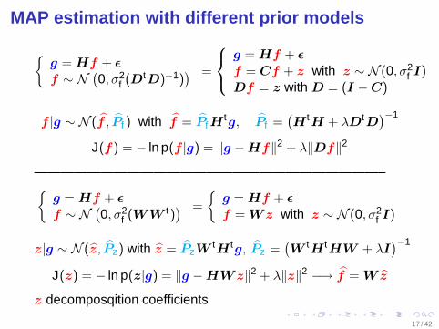
MAP estimation with different prior models

g = Hf + ǫ

f ∼ N(0, σ2

f (DtD)−1)) =

g = Hf + ǫ

f = Cf + z with z ∼ N (0, σ2f I)

Df = z with D = (I − C)

f |g ∼ N (f , Pf ) with f = Pf Htg, Pf =

(H tH + λDtD

)−1

J(f ) = − ln p(f |g) = ‖g − Hf‖2 + λ‖Df‖2

——————————————————————————–

g = Hf + ǫ

f ∼ N(0, σ2

f (WW t)) =

g = Hf + ǫ

f = Wz with z ∼ N (0, σ2f I)

z|g ∼ N (z, Pz) with z = PzWtH tg, Pz =

(W tH tHW + λI

)−1

J(z) = − ln p(z|g) = ‖g − HWz‖2 + λ‖z‖2 −→ f = Wz

z decomposqition coefficients

17 / 42

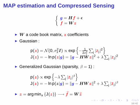
MAP estimation and Compressed Sensing

g = Hf + ǫ

f = Wz

W a code book matrix, z coefficients Gaussian :

p(z) = N (0, σ2zI) ∝ exp

− 1

2σ2z

∑j |z j |

2

J(z) = − ln p(z|g) = ‖g − HWz‖2 + λ∑

j |z j |2

Generalized Gaussian (sparsity, β = 1) :

p(z) ∝ exp−λ

∑j |z j |

β

J(z) = − ln p(z|g) = ‖g − HWz‖2 + λ∑

j |z j |β

z = arg minz J(z) −→ f = Wz

18 / 42

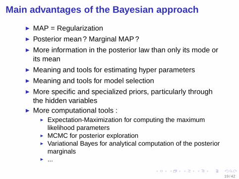
Main advantages of the Bayesian approach

MAP = Regularization Posterior mean ? Marginal MAP ? More information in the posterior law than only its mode or

its mean Meaning and tools for estimating hyper parameters Meaning and tools for model selection More specific and specialized priors, particularly through

the hidden variables More computational tools :

Expectation-Maximization for computing the maximumlikelihood parameters

MCMC for posterior exploration Variational Bayes for analytical computation of the posterior

marginals ...

19 / 42

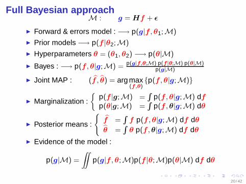
Full Bayesian approachM : g = Hf + ǫ

Forward & errors model : −→ p(g|f ,θ1;M)

Prior models −→ p(f |θ2;M)

Hyperparameters θ = (θ1,θ2) −→ p(θ|M)

Bayes : −→ p(f ,θ|g;M) = p(g|f,θ;M) p(f|θ;M) p(θ|M)p(g|M)

Joint MAP : (f , θ) = arg max(f ,θ)

p(f ,θ|g;M)

Marginalization :

p(f |g;M) =∫∫

p(f ,θ|g;M) df

p(θ|g;M) =∫∫

p(f ,θ|g;M) dθ

Posterior means :

f =

∫∫f p(f ,θ|g;M) df dθ

θ =∫∫

θ p(f ,θ|g;M) df dθ

Evidence of the model :

p(g|M) =

∫∫p(g|f ,θ;M)p(f |θ;M)p(θ|M) df dθ

20 / 42

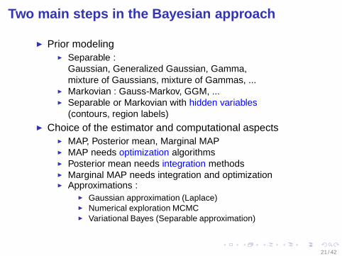
Two main steps in the Bayesian approach

Prior modeling Separable :

Gaussian, Generalized Gaussian, Gamma,mixture of Gaussians, mixture of Gammas, ...

Markovian : Gauss-Markov, GGM, ... Separable or Markovian with hidden variables

(contours, region labels) Choice of the estimator and computational aspects

MAP, Posterior mean, Marginal MAP MAP needs optimization algorithms Posterior mean needs integration methods Marginal MAP needs integration and optimization Approximations :

Gaussian approximation (Laplace) Numerical exploration MCMC Variational Bayes (Separable approximation)

21 / 42

Which images I am looking for ?

50 100 150 200 250 300

50

100

150

200

250

300

350

400

450

22 / 42

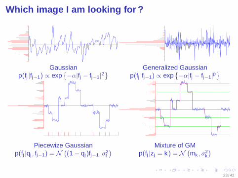
Which image I am looking for ?

Gaussian Generalized Gaussianp(fj |fj−1) ∝ exp

−α|fj − fj−1|

2

p(fj |fj−1) ∝ exp−α|fj − fj−1|

p

Piecewize Gaussian Mixture of GMp(fj |qj , fj−1) = N

((1 − qj)fj−1, σ

2f

)p(fj |zj = k) = N

(mk , σ2

k

)

23 / 42

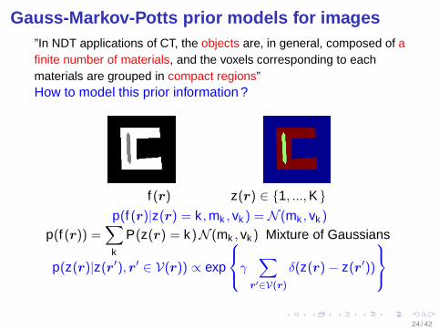
Gauss-Markov-Potts prior models for images”In NDT applications of CT, the objects are, in general, composed of afinite number of materials, and the voxels corresponding to eachmaterials are grouped in compact regions”How to model this prior information ?

f (r) z(r) ∈ 1, ..., K

p(f (r)|z(r) = k , mk , vk ) = N (mk , vk )

p(f (r)) =∑

k

P(z(r) = k)N (mk , vk ) Mixture of Gaussians

p(z(r)|z(r′), r′ ∈ V(r)) ∝ exp

γ∑

r′∈V(r)

δ(z(r) − z(r′))

24 / 42

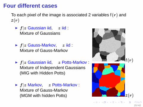
Four different cases

To each pixel of the image is associated 2 variables f (r) andz(r)

f |z Gaussian iid, z iid :Mixture of Gaussians

f |z Gauss-Markov, z iid :Mixture of Gauss-Markov

f |z Gaussian iid, z Potts-Markov :Mixture of Independent Gaussians(MIG with Hidden Potts)

f |z Markov, z Potts-Markov :Mixture of Gauss-Markov(MGM with hidden Potts)

f (r)

z(r)

25 / 42

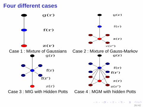
Four different cases

Case 1 : Mixture of Gaussians Case 2 : Mixture of Gauss-Markov

Case 3 : MIG with Hidden Potts Case 4 : MGM with hidden Potts

26 / 42

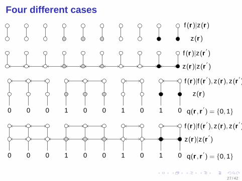
Four different cases

f (r )|z(r)

z(r)

f (r )|z(r′

)

z(r)|z(r′

)

0 0 0 0 0 0 01 1 1

f (r)|f (r′

), z(r), z(r′

)

z(r)

q(r , r′

) = 0, 1

0 0 0 0 0 0 01 1 1

f (r)|f (r′

), z(r), z(r′

)

z(r)|z(r′

)

q(r , r′

) = 0, 1

27 / 42

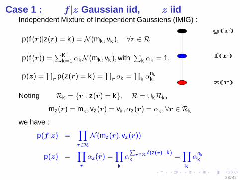
Case 1 : f |z Gaussian iid, z iidIndependent Mixture of Independent Gaussiens (IMIG) :

p(f (r)|z(r) = k) = N (mk , vk ), ∀r ∈ R

p(f (r)) =∑K

k=1 αkN (mk , vk ), with∑

k αk = 1.

p(z) =∏

r p(z(r) = k) =∏

r αk =∏

k αnkk

Noting Rk = r : z(r) = k, R = ∪kRk ,

mz(r) = mk , vz(r) = vk , αz(r) = αk ,∀r ∈ Rk

we have :

p(f |z) =∏

r∈R

N (mz(r), vz (r))

p(z) =∏

r

αz(r) =∏

k

αP

r∈Rδ(z(r)−k)

k =∏

k

αnkk

28 / 42

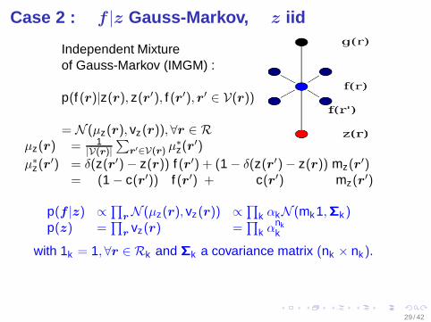
Case 2 : f |z Gauss-Markov, z iid

Independent Mixtureof Gauss-Markov (IMGM) :

p(f (r)|z(r), z(r′), f (r′), r′ ∈ V(r))

= N (µz(r), vz (r)),∀r ∈ Rµz(r) = 1

|V(r)|

∑r′∈V(r) µ∗

z(r′)

µ∗z(r

′) = δ(z(r′) − z(r)) f (r′) + (1 − δ(z(r′) − z(r)) mz(r′)

= (1 − c(r′)) f (r′) + c(r′) mz(r′)

p(f |z) ∝∏

r N (µz(r), vz (r)) ∝∏

k αkN (mk1,Σk )

p(z) =∏

r vz(r) =∏

k αnkk

with 1k = 1,∀r ∈ Rk and Σk a covariance matrix (nk × nk).

29 / 42

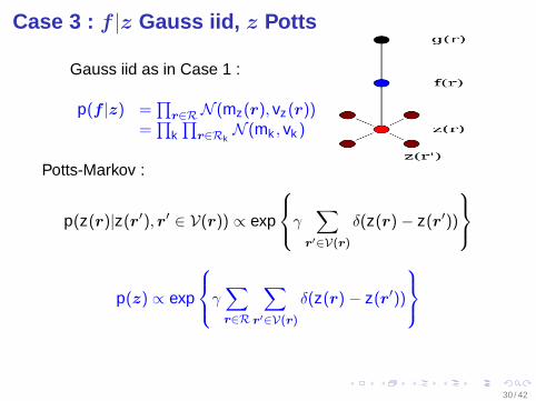
Case 3 : f |z Gauss iid, z Potts

Gauss iid as in Case 1 :

p(f |z) =∏

r∈R N (mz(r), vz (r))=

∏k∏

r∈RkN (mk , vk )

Potts-Markov :

p(z(r)|z(r′), r′ ∈ V(r)) ∝ exp

γ∑

r′∈V(r)

δ(z(r) − z(r′))

p(z) ∝ exp

γ∑

r∈R

∑

r′∈V(r)

δ(z(r) − z(r′))

30 / 42

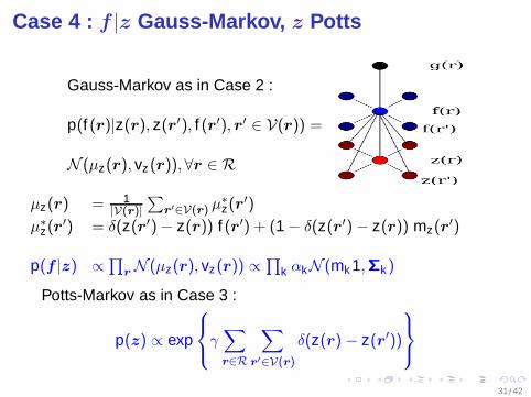
Case 4 : f |z Gauss-Markov, z Potts

Gauss-Markov as in Case 2 :

p(f (r)|z(r), z(r′), f (r′), r′ ∈ V(r)) =

N (µz(r), vz (r)),∀r ∈ R

µz(r) = 1|V(r)|

∑r′∈V(r) µ∗

z(r′)

µ∗z(r

′) = δ(z(r′) − z(r)) f (r′) + (1 − δ(z(r′) − z(r)) mz(r′)

p(f |z) ∝∏

r N (µz(r), vz(r)) ∝∏

k αkN (mk1,Σk )

Potts-Markov as in Case 3 :

p(z) ∝ exp

γ∑

r∈R

∑

r′∈V(r)

δ(z(r) − z(r′))

31 / 42

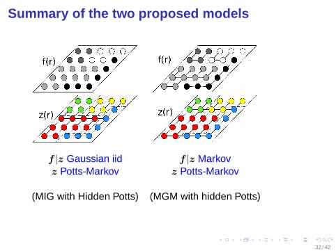
Summary of the two proposed models

f |z Gaussian iid f |z Markovz Potts-Markov z Potts-Markov

(MIG with Hidden Potts) (MGM with hidden Potts)

32 / 42

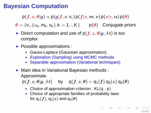
Bayesian Computation

p(f ,z,θ|g) ∝ p(g|f ,z, vǫ) p(f |z,m,v) p(z|γ,α) p(θ)

θ = vǫ, (αk , mk , vk ), k = 1, ·, K p(θ) Conjugate priors

Direct computation and use of p(f ,z,θ|g;M) is toocomplex

Possible approximations : Gauss-Laplace (Gaussian approximation) Exploration (Sampling) using MCMC methods Separable approximation (Variational techniques)

Main idea in Variational Bayesian methods :Approximatep(f ,z,θ|g;M) by q(f ,z,θ) = q1(f) q2(z) q3(θ)

Choice of approximation criterion : KL(q : p) Choice of appropriate families of probability laws

for q1(f), q2(z) and q3(θ)

33 / 42

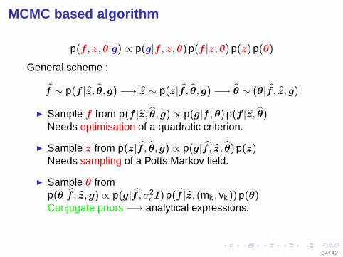
MCMC based algorithm

p(f ,z,θ|g) ∝ p(g|f ,z,θ) p(f |z,θ) p(z) p(θ)

General scheme :

f ∼ p(f |z, θ,g) −→ z ∼ p(z|f , θ,g) −→ θ ∼ (θ|f , z,g)

Sample f from p(f |z, θ,g) ∝ p(g|f ,θ) p(f |z, θ)Needs optimisation of a quadratic criterion.

Sample z from p(z|f , θ,g) ∝ p(g|f , z, θ) p(z)Needs sampling of a Potts Markov field.

Sample θ fromp(θ|f , z,g) ∝ p(g|f , σ2

ǫ I) p(f |z, (mk , vk )) p(θ)Conjugate priors −→ analytical expressions.

34 / 42

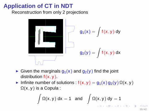
Application of CT in NDTReconstruction from only 2 projections

g1(x) =

∫f (x , y) dy

g2(y) =

∫f (x , y) dx

Given the marginals g1(x) and g2(y) find the jointdistribution f (x , y).

Infinite number of solutions : f (x , y) = g1(x) g2(y) Ω(x , y)Ω(x , y) is a Copula :

∫Ω(x , y) dx = 1 and

∫Ω(x , y) dy = 1

35 / 42

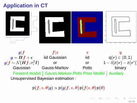
Application in CT

20 40 60 80 100 120

20

40

60

80

100

120

g|f f |z z q

g = Hf + ǫ iid Gaussian iid q(r) ∈ 0, 1g|f ∼ N (Hf , σ2

ǫ I) or or 1 − δ(z(r) − z(r′))Gaussian Gauss-Markov Potts binaryForward model Gauss-Markov-Potts Prior Model Auxilary

Unsupervised Bayesian estimation :

p(f ,z,θ|g) ∝ p(g|f ,z,θ) p(f |z,θ) p(θ)

36 / 42

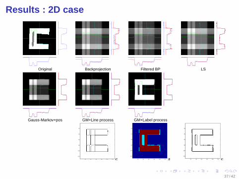
Results : 2D case

Original Backprojection Filtered BP LS

Gauss-Markov+pos GM+Line process GM+Label process

20 40 60 80 100 120

20

40

60

80

100

120

c 20 40 60 80 100 120

20

40

60

80

100

120

z 20 40 60 80 100 120

20

40

60

80

100

120

c

37 / 42

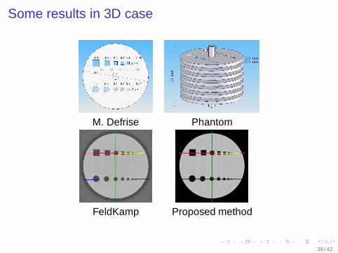
Some results in 3D case

M. Defrise Phantom

FeldKamp Proposed method

38 / 42

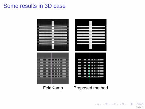
Some results in 3D case

FeldKamp Proposed method

39 / 42

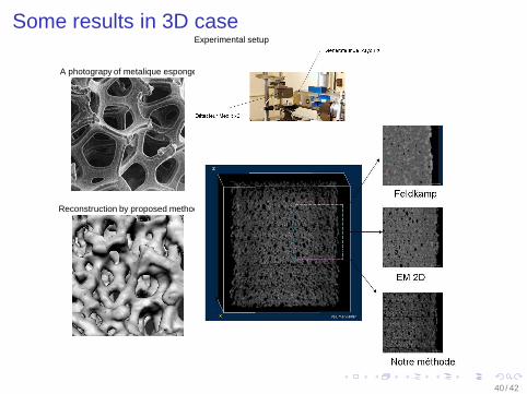
Some results in 3D case

A photograpy of metalique esponge

Reconstruction by proposed method

Experimental setup

40 / 42

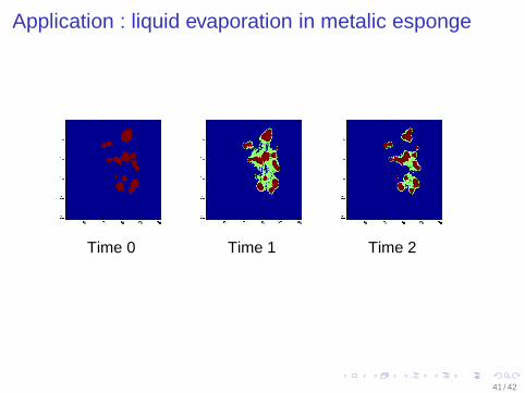
Application : liquid evaporation in metalic esponge

Time 0 Time 1 Time 2

41 / 42

Conclusions

Bayesian estimation approach gives more tools thandeterministic regularization to handle inverses problems

Gauss-Markov-Potts are useful prior models for imagesincorporating regions and contours

Bayesian computation needs either multi-dimensionaloptimization or integration methods

Different optimization and integration tools andapproximations exist (Laplace, MCMC, Variational Bayes)

Work in Progress and Perspectives : Efficient implementation in 2D and 3D cases using GPU Application to other linear and non linear inverse

problems : X ray CT, Ultrasound and Microwave imaging,PET, SPECT, ...

42 / 42