Introduction to Bayesian inference

Thomas Alexander Brouwer

University of Cambridge

tab43@cam.ac.uk

17 November 2015

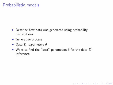
Probabilistic models

I Describe how data was generated using probabilitydistributions

I Generative process

I Data D, parameters θ

I Want to find the “best” parameters θ for the data D -inference

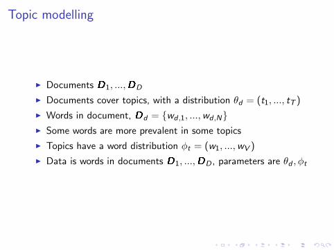
Topic modelling

I Documents D1, ...,DD

I Documents cover topics, with a distribution θd = (t1, ..., tT )

I Words in document, Dd = {wd ,1, ...,wd ,N}I Some words are more prevalent in some topics

I Topics have a word distribution φt = (w1, ...,wV )

I Data is words in documents D1, ...,DD , parameters are θd , φt

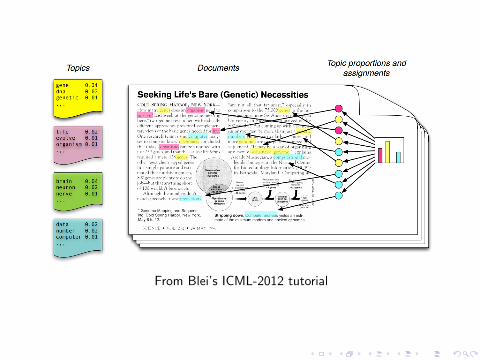
From Blei’s ICML-2012 tutorial

Overview

Probabilistic modelsProbability theoryLatent variable models

Bayesian inferenceBayes’ theoremLatent Dirichlet AllocationConjugacy

Graphical models

Gibbs sampling

Variational Bayesian inference

Probability primer

I Random variable X

I Probability distribution p(X )

I Discrete distribution – e.g. coin flip or dice roll

I Continuous distribution – e.g. height distribution

Multiple RVs

I Joint distribution p(X ,Y )

I Conditional distribution p(X |Y )

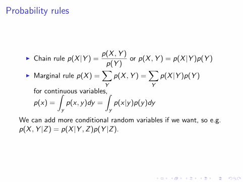
Probability rules

I Chain rule p(X |Y ) =p(X ,Y )

p(Y )or p(X ,Y ) = p(X |Y )p(Y )

I Marginal rule p(X ) =∑Y

p(X ,Y ) =∑Y

p(X |Y )p(Y )

for continuous variables,

p(x) =

∫yp(x , y)dy =

∫yp(x |y)p(y)dy

We can add more conditional random variables if we want, so e.g.p(X ,Y |Z ) = p(X |Y ,Z )p(Y |Z ).

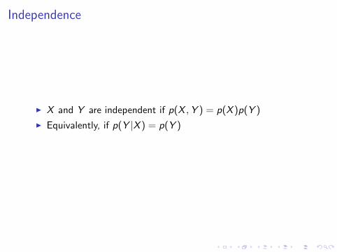
Independence

I X and Y are independent if p(X ,Y ) = p(X )p(Y )

I Equivalently, if p(Y |X ) = p(Y )

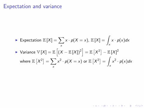
Expectation and variance

I Expectation E [X ] =∑x

x · p(X = x), E [X ] =

∫xx · p(x)dx

I Variance V [X ] = E[(X − E [X ])2

]= E

[X 2]− E [X ]2

where E[X 2]

=∑x

x2 · p(X = x) or E[X 2]

=

∫xx2 · p(x)dx

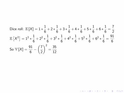
Dice roll: E [X ] = 1 ∗ 1

6+ 2 ∗ 1

6+ 3 ∗ 1

6+ 4 ∗ 1

6+ 5 ∗ 1

6+ 6 ∗ 1

6=

7

2

E[X 2]

= 12 ∗ 1

6+ 22 ∗ 1

6+ 32 ∗ 1

6+ 42 ∗ 1

6+ 52 ∗ 1

6+ 62 ∗ 1

6=

91

6

So V [X ] =91

6−(

7

2

)2

=35

12

Latent variable models

I Manifest or observed variable

I Latent or unobserved variable

I Latent variable models

Probability distributions

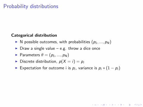
Categorical distribution

I N possible outcomes, with probabilities (p1, ..., pN)

I Draw a single value – e.g. throw a dice once

I Parameters θ = (p1, ..., pN)

I Discrete distribution, p(X = i) = piI Expectation for outcome i is pi , variance is pi ∗ (1− pi )

Probability distributions

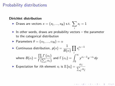
Dirichlet distribution

I Draws are vectors x = (x1, ..., xN) s.t.∑i

xi = 1

I In other words, draws are probability vectors – the parameterto the categorical distribution

I Parameters θ = (α1, ..., αN) = α

I Continuous distribution, p(x) =1

B(α)

∏i

xαi−1i

where B(α) =

∏i Γ (αi )

Γ (∑

i αi )and Γ (αi ) =

∫ ∞0

yαi−1e−αidy

I Expectation for ith element xi is E [xi ] =αi∑j αj

Probabilistic modelsProbability theoryLatent variable models

Bayesian inferenceBayes’ theoremLatent Dirichlet AllocationConjugacy

Graphical models

Gibbs sampling

Variational Bayesian inference

Unfair dice

I Dice with unknown distribution, p = (p1, p2, p3, p4, p5, p6)

I We observe some throws and want to estimate p

I Say we observe 4, 6, 6, 4, 6, 3

I Perhaps p = (0, 0, 16 ,26 , 0,

36)

Maximum likelihood

I Maximum likelihood solution, θML = maxθ

p(D|θ)

I Easily leads to overfitting

I Want to incorporate some prior belief or knowledge about ourparameters

Bayes’ theorem

Bayes’ theoremFor any two random variables X and Y ,

p(X |Y ) =p(Y |X )p(X )

p(Y )

ProofFrom chain rule, p(X ,Y ) = p(Y |X )p(X ) = p(X |Y )p(Y ).Divide both sides by p(Y ).

Disease test

I Test for disease with 99% accuracy

I 1 in a 1000 people have the disease

I You tested positive. What is the probability that you have thedisease?

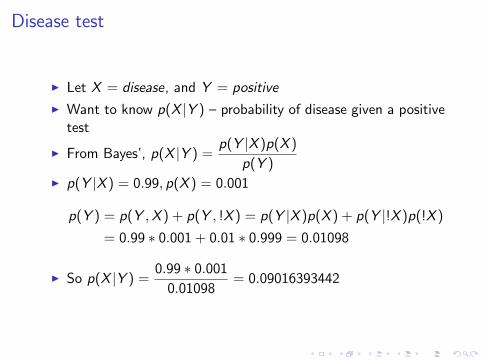
Disease test

I Let X = disease, and Y = positive

I Want to know p(X |Y ) – probability of disease given a positivetest

I From Bayes’, p(X |Y ) =p(Y |X )p(X )

p(Y )I p(Y |X ) = 0.99, p(X ) = 0.001

p(Y ) = p(Y ,X ) + p(Y , !X ) = p(Y |X )p(X ) + p(Y |!X )p(!X )

= 0.99 ∗ 0.001 + 0.01 ∗ 0.999 = 0.01098

I So p(X |Y ) =0.99 ∗ 0.001

0.01098= 0.09016393442

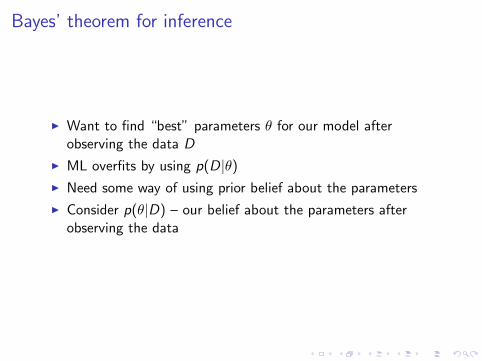
Bayes’ theorem for inference

I Want to find “best” parameters θ for our model afterobserving the data D

I ML overfits by using p(D|θ)

I Need some way of using prior belief about the parameters

I Consider p(θ|D) – our belief about the parameters afterobserving the data

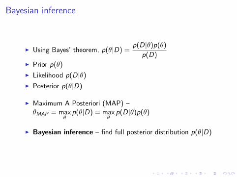
Bayesian inference

I Using Bayes’ theorem, p(θ|D) =p(D|θ)p(θ)

p(D)I Prior p(θ)

I Likelihood p(D|θ)

I Posterior p(θ|D)

I Maximum A Posteriori (MAP) –θMAP = max

θp(θ|D) = max

θp(D|θ)p(θ)

I Bayesian inference – find full posterior distribution p(θ|D)

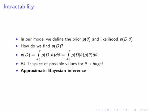
Intractability

I In our model we define the prior p(θ) and likelihood p(D|θ)

I How do we find p(D)?

I p(D) =

∫θp(D, θ)dθ =

∫θp(D|θ)p(θ)dθ

I BUT: space of possible values for θ is huge!

I Approximate Bayesian inference

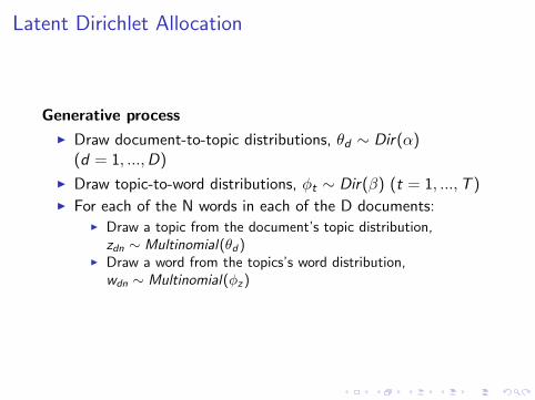
Latent Dirichlet Allocation

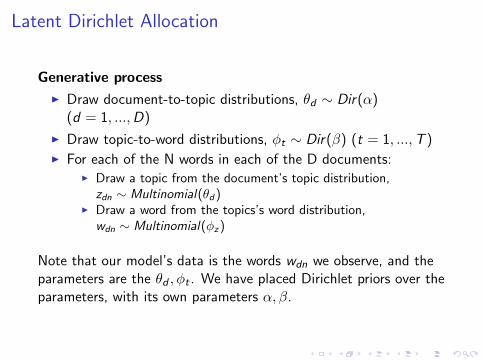
Generative process

I Draw document-to-topic distributions, θd ∼ Dir(α)(d = 1, ...,D)

I Draw topic-to-word distributions, φt ∼ Dir(β) (t = 1, ...,T )I For each of the N words in each of the D documents:

I Draw a topic from the document’s topic distribution,zdn ∼ Multinomial(θd)

I Draw a word from the topics’s word distribution,wdn ∼ Multinomial(φz)

Note that our model’s data is the words wdn we observe, and theparameters are the θd , φt . We have placed Dirichlet priors over theparameters, with its own parameters α, β.

Hyperparameters

In our model we have:

I Random variables – observed ones, like the words; and latentones, like the topics

I Parameters – document-to-topic distributions θd andtopic-to-word distributions φd

I Hyperparameters – these are parameters to the priordistributions over our parameters, so α and β

Conjugacy

For a specific parameter θi , p(θi ) is conjugate to the likelihoodp(D|θi ) if the posterior of the parameter, p(θi |D), is of the samefamily as the prior.

e.g. the Dirichlet distribution is the conjugate prior for thecategorical distribution.

Probabilistic modelsProbability theoryLatent variable models

Bayesian inferenceBayes’ theoremLatent Dirichlet AllocationConjugacy

Graphical models

Gibbs sampling

Variational Bayesian inference

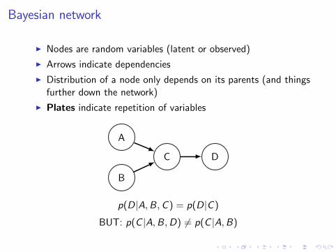
Bayesian network

I Nodes are random variables (latent or observed)

I Arrows indicate dependencies

I Distribution of a node only depends on its parents (and thingsfurther down the network)

I Plates indicate repetition of variables

A

B

C D

p(D|A,B,C ) = p(D|C )

BUT: p(C |A,B,D) 6= p(C |A,B)

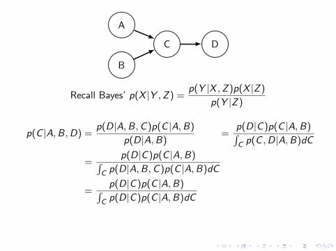
A

B

C D

Recall Bayes’ p(X |Y ,Z ) =p(Y |X ,Z )p(X |Z )

p(Y |Z )

p(C |A,B,D) =p(D|A,B,C )p(C |A,B)

p(D|A,B)=

p(D|C )p(C |A,B)∫C p(C ,D|A,B)dC

=p(D|C )p(C |A,B)∫

C p(D|A,B,C )p(C |A,B)dC

=p(D|C )p(C |A,B)∫

C p(D|C )p(C |A,B)dC

Latent Dirichlet Allocation

Generative process

I Draw document-to-topic distributions, θd ∼ Dir(α)(d = 1, ...,D)

I Draw topic-to-word distributions, φt ∼ Dir(β) (t = 1, ...,T )I For each of the N words in each of the D documents:

I Draw a topic from the document’s topic distribution,zdn ∼ Multinomial(θd)

I Draw a word from the topics’s word distribution,wdn ∼ Multinomial(φz)

Latent Dirichlet Allocation

From http://parkcu.com/blog/

Probabilistic modelsProbability theoryLatent variable models

Bayesian inferenceBayes’ theoremLatent Dirichlet AllocationConjugacy

Graphical models

Gibbs sampling

Variational Bayesian inference

Gibbs sampling

I Want to approximate p(θ|D) for parameters θ = (θ1, ..., θN)

I Cannot compute this exactly, but maybe we can draw samplesfrom it

I We can then use these samples to estimate the distribution, orestimate the expectation and variance

Gibbs sampling

I For each parameter θi , write down its distribution conditionalon the data and the values of the other parameters,p(θi |θ−i ,D)

I If our model is conjugate, this gives closed-form expressions(meaning this distribution is of a known form, e.g. Dirichlet,so we can draw from it)

I Drawing new values for the parameters θi in turn willeventually converge to give draws from the true posterior,p(θ|D)

I Burn-in, thinning

Latent Dirichlet Allocation

I Want to draw samples from p(θ,φ, z |w)

I w = {wd ,n}d=1..D,n=1..N

I z = {zd ,n}d=1..D,n=1..N

I θ = {θd}d=1..D

I φ = {φt}t=1..T

Latent Dirichlet Allocation

For Gibbs sampling, need distribitions:

I p(θd |θ−d ,φ, z ,w)

I p(φt |θ,φ−t , z ,w)

I p(zd ,n|θ,φ, z−d ,n,w)

Latent Dirichlet Allocation

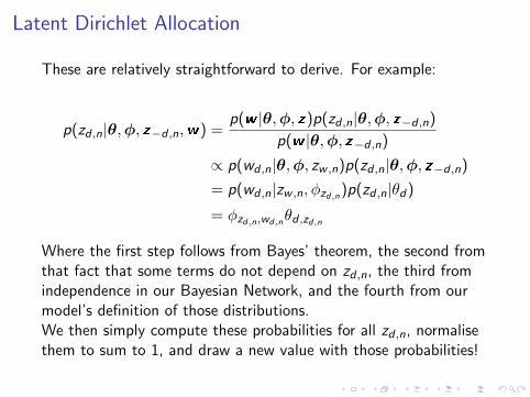
These are relatively straightforward to derive. For example:

p(zd ,n|θ,φ, z−d ,n,w) =p(w |θ,φ, z)p(zd ,n|θ,φ, z−d ,n)

p(w |θ,φ, z−d ,n)

∝ p(wd ,n|θ,φ, zw ,n)p(zd ,n|θ,φ, z−d ,n)

= p(wd ,n|zw ,n, φzd,n)p(zd ,n|θd)

= φzd,n,wd,nθd ,zd,n

Where the first step follows from Bayes’ theorem, the second fromthat fact that some terms do not depend on zd ,n, the third fromindependence in our Bayesian Network, and the fourth from ourmodel’s definition of those distributions.We then simply compute these probabilities for all zd ,n, normalisethem to sum to 1, and draw a new value with those probabilities!

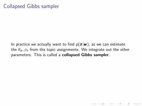
Collapsed Gibbs sampler

In practice we actually want to find p(z |w), as we can estimatethe θd , φt from the topic assignments. We integrate out the otherparameters. This is called a collapsed Gibbs sampler.

Probabilistic modelsProbability theoryLatent variable models

Bayesian inferenceBayes’ theoremLatent Dirichlet AllocationConjugacy

Graphical models

Gibbs sampling

Variational Bayesian inference

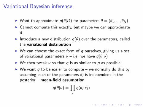
Variational Bayesian inference

I Want to approximate p(θ|D) for parameters θ = (θ1, ..., θN)

I Cannot compute this exactly, but maybe we can approximateit

I Introduce a new distribution q(θ) over the parameters, calledthe variational distribution

I We can choose the exact form of q ourselves, giving us a setof variational parameters ν – i.e. we have q(θ|ν)

I We then tweak ν so that q is as similar to p as possible!

I We want q to be easier to compute – we normally do this byassuming each of the parameters θi is independent in theposterior – mean-field assumption

q(θ|ν) =∏i

q(θi |νi )

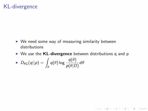
KL-divergence

I We need some way of measuring similarity betweendistributions

I We use the KL-divergence between distributions q and p

I DKL(q||p) =

∫θq(θ) log

q(θ)

p(θ|D)dθ

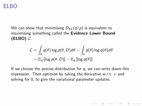
ELBO

We can show that minimising DKL(q||p) is equivalent tomaximising something called the Evidence Lower Bound(ELBO) L.

L =

∫θq(θ) log p(θ,D)dθ −

∫θq(θ) log q(θ)dθ

= Eq [log p(θ,D)]− Eq [log q(θ)]

If we choose the precise distribution for q, we can write down thisexpression. Then optimise by taking the derivative w.r.t. ν andsolving for 0, to give the variational parameter updates.

Convergence

We update the variational parameters ν in turn, and alternateupdates until the value of the ELBO converges.

After convergence, our estimate of the posterior distribution of aparameter θi is q(θi |νi ).

Choosing q

I Our choice of q determines how well our approximation to p is

I If our model has conjugacy, we simply choose the samedistribution for q(θi ) as we used for Gibbs sampling,p(θi |θ−i ,D)

I We then obtain very nice updates

I In non-conjugate models we need to use gradient descent tooptimise the ELBO!

Introduction to Bayesian inference

Thomas Alexander Brouwer

University of Cambridge

tab43@cam.ac.uk

17 November 2015