


γλώσσες
Σελίδες
Νομικός

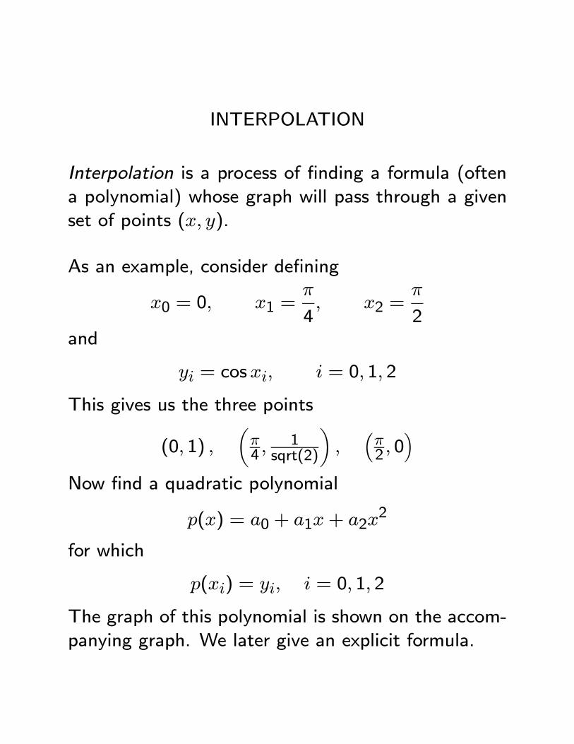
INTERPOLATION
Interpolation is a process of finding a formula (oftena polynomial) whose graph will pass through a givenset of points (x, y).
As an example, consider defining
x0 = 0, x1 =π
4, x2 =
π
2and
yi = cosxi, i = 0, 1, 2
This gives us the three points
(0, 1) ,µπ4 ,
1sqrt(2)
¶,
³π2 , 0
´Now find a quadratic polynomial
p(x) = a0 + a1x+ a2x2
for which
p(xi) = yi, i = 0, 1, 2
The graph of this polynomial is shown on the accom-panying graph. We later give an explicit formula.
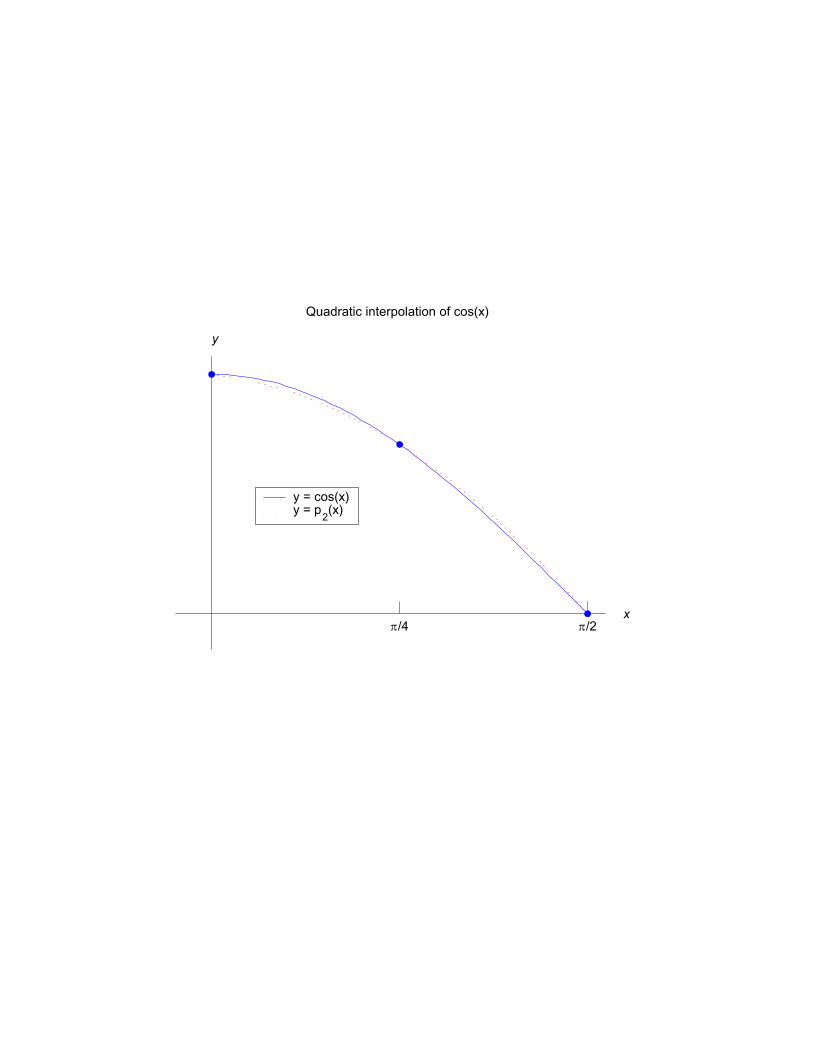
Quadratic interpolation of cos(x)
x
y
π/4 π/2
y = cos(x)y = p2(x)
PURPOSES OF INTERPOLATION
1. Replace a set of data points {(xi, yi)} with a func-tion given analytically.
2. Approximate functions with simpler ones, usually
polynomials or ‘piecewise polynomials’.
Purpose #1 has several aspects.
• The data may be from a known class of functions.Interpolation is then used to find the member of
this class of functions that agrees with the given
data. For example, data may be generated from
functions of the form
p(x) = a0 + a1ex + a2e
2x + · · ·+ anenx
Then we need to find the coefficientsnajobased
on the given data values.
• We may want to take function values f(x) givenin a table for selected values of x, often equally
spaced, and extend the function to values of x
not in the table.
For example, given numbers from a table of loga-
rithms, estimate the logarithm of a number x not
in the table.
• Given a set of data points {(xi, yi)}, find a curvepassing thru these points that is “pleasing to the
eye”. In fact, this is what is done continually with
computer graphics. How do we connect a set of
points to make a smooth curve? Connecting them
with straight line segments will often give a curve
with many corners, whereas what was intended
was a smooth curve.
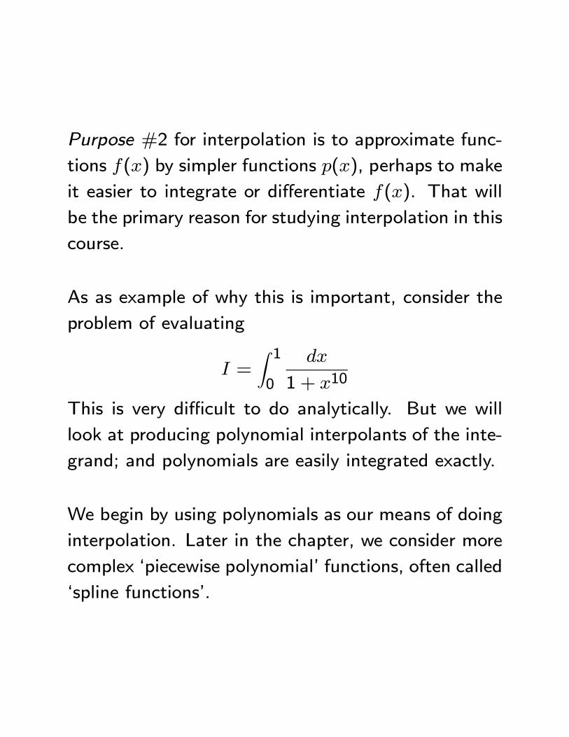
Purpose #2 for interpolation is to approximate func-
tions f(x) by simpler functions p(x), perhaps to make
it easier to integrate or differentiate f(x). That will
be the primary reason for studying interpolation in this
course.
As as example of why this is important, consider the
problem of evaluating
I =Z 10
dx
1 + x10
This is very difficult to do analytically. But we will
look at producing polynomial interpolants of the inte-
grand; and polynomials are easily integrated exactly.
We begin by using polynomials as our means of doing
interpolation. Later in the chapter, we consider more
complex ‘piecewise polynomial’ functions, often called
‘spline functions’.
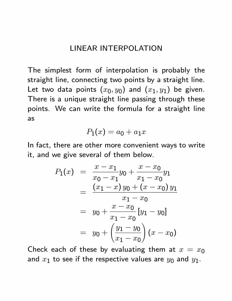
LINEAR INTERPOLATION
The simplest form of interpolation is probably thestraight line, connecting two points by a straight line.
Let two data points (x0, y0) and (x1, y1) be given.
There is a unique straight line passing through these
points. We can write the formula for a straight lineas
P1(x) = a0 + a1x
In fact, there are other more convenient ways to write
it, and we give several of them below.
P1(x) =x− x1x0 − x1
y0 +x− x0x1 − x0
y1
=(x1 − x) y0 + (x− x0) y1
x1 − x0
= y0 +x− x0x1 − x0
[y1 − y0]
= y0 +
Ãy1 − y0x1 − x0
!(x− x0)
Check each of these by evaluating them at x = x0and x1 to see if the respective values are y0 and y1.

Example. Following is a table of values for f(x) =tanx for a few values of x.
x 1 1.1 1.2 1.3tanx 1.5574 1.9648 2.5722 3.6021
Use linear interpolation to estimate tan(1.15). Then
use
x0 = 1.1, x1 = 1.2
with corresponding values for y0 and y1. Then
tanx ≈ y0 +x− x0x1 − x0
[y1 − y0]
tanx ≈ y0 +x− x0x1 − x0
[y1 − y0]
tan (1.15) ≈ 1.9648 +1.15− 1.11.2− 1.1 [2.5722− 1.9648]
= 2.2685
The true value is tan 1.15 = 2.2345. We will want
to examine formulas for the error in interpolation, to
know when we have sufficient accuracy in our inter-
polant.
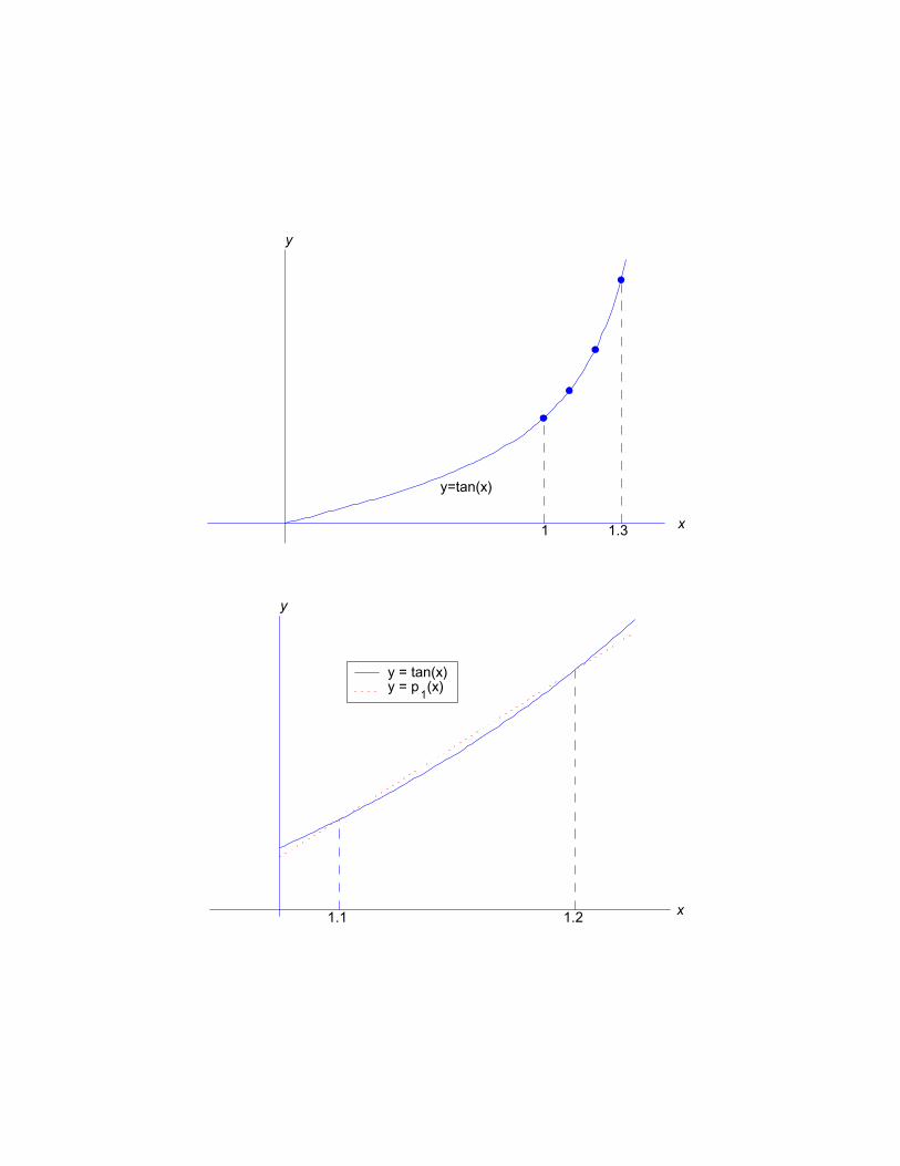
x
y
1 1.3
y=tan(x)
x
y
1.1 1.2
y = tan(x)y = p1(x)
QUADRATIC INTERPOLATION
We want to find a polynomial
P2(x) = a0 + a1x+ a2x2
which satisfies
P2(xi) = yi, i = 0, 1, 2
for given data points (x0, y0) , (x1, y1) , (x2, y2). One
formula for such a polynomial follows:
P2(x) = y0L0(x) + y1L1(x) + y2L2(x) (∗∗)with
L0(x) =(x−x1)(x−x2)(x0−x1)(x0−x2), L1(x) =
(x−x0)(x−x2)(x1−x0)(x1−x2)
L2(x) =(x−x0)(x−x1)(x2−x0)(x2−x1)
The formula (∗∗) is called Lagrange’s form of the in-
terpolation polynomial.
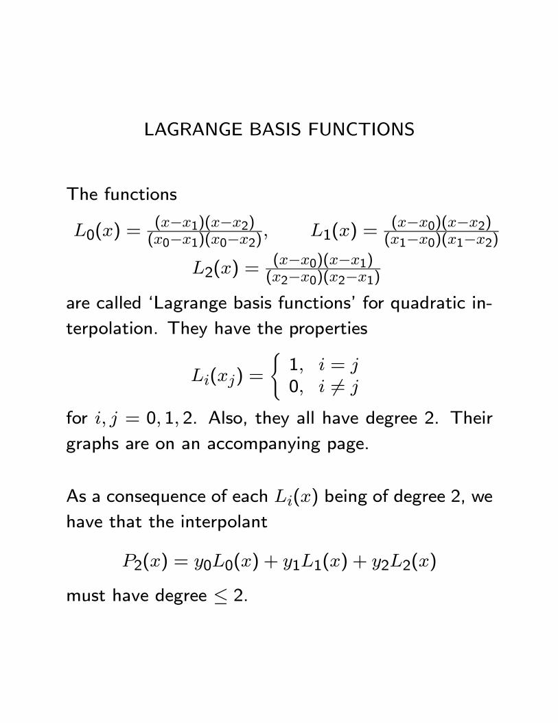
LAGRANGE BASIS FUNCTIONS
The functions
L0(x) =(x−x1)(x−x2)(x0−x1)(x0−x2), L1(x) =
(x−x0)(x−x2)(x1−x0)(x1−x2)
L2(x) =(x−x0)(x−x1)(x2−x0)(x2−x1)
are called ‘Lagrange basis functions’ for quadratic in-
terpolation. They have the properties
Li(xj) =
(1, i = j0, i 6= j
for i, j = 0, 1, 2. Also, they all have degree 2. Their
graphs are on an accompanying page.
As a consequence of each Li(x) being of degree 2, we
have that the interpolant
P2(x) = y0L0(x) + y1L1(x) + y2L2(x)
must have degree ≤ 2.
UNIQUENESS
Can there be another polynomial, call it Q(x), forwhich
deg(Q) ≤ 2Q(xi) = yi, i = 0, 1, 2
Thus, is the Lagrange formula P2(x) unique?
Introduce
R(x) = P2(x)−Q(x)
From the properties of P2 and Q, we have deg(R) ≤2. Moreover,
R(xi) = P2(xi)−Q(xi) = yi − yi = 0
for all three node points x0, x1, and x2. How manypolynomials R(x) are there of degree at most 2 andhaving three distinct zeros? The answer is that onlythe zero polynomial satisfies these properties, and there-fore
R(x) = 0 for all x
Q(x) = P2(x) for all x
SPECIAL CASES
Consider the data points
(x0, 1), (x1, 1), (x2, 1)
What is the polynomial P2(x) in this case?
Answer: We must have the polynomial interpolant is
P2(x) ≡ 1meaning that P2(x) is the constant function. Why?First, the constant function satisfies the property ofbeing of degree ≤ 2. Next, it clearly interpolates thegiven data. Therefore by the uniqueness of quadraticinterpolation, P2(x) must be the constant function 1.
Consider now the data points
(x0,mx0), (x1,mx1), (x2,mx2)
for some constant m. What is P2(x) in this case? Byan argument similar to that above,
P2(x) = mx for all x
Thus the degree of P2(x) can be less than 2.
HIGHER DEGREE INTERPOLATION
We consider now the case of interpolation by poly-nomials of a general degree n. We want to find apolynomial Pn(x) for which
deg(Pn) ≤ nPn(xi) = yi, i = 0, 1, · · · , n (∗∗)
with given data points
(x0, y0) , (x1, y1) , · · · , (xn, yn)The solution is given by Lagrange’s formula
Pn(x) = y0L0(x) + y1L1(x) + · · ·+ ynLn(x)
The Lagrange basis functions are given by
Lk(x) =(x− x0) ..(x− xk−1)(x− xk+1).. (x− xn)
(xk − x0) ..(xk − xk−1)(xk − xk+1).. (xk − xn)
for k = 0, 1, 2, ..., n. The quadratic case was coveredearlier.
In a manner analogous to the quadratic case, we canshow that the above Pn(x) is the only solution to theproblem (∗∗).
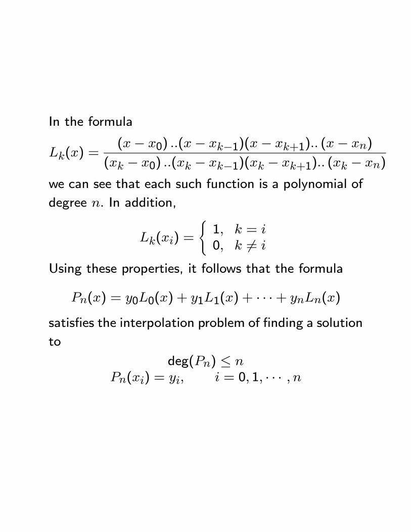
In the formula
Lk(x) =(x− x0) ..(x− xk−1)(x− xk+1).. (x− xn)
(xk − x0) ..(xk − xk−1)(xk − xk+1).. (xk − xn)
we can see that each such function is a polynomial of
degree n. In addition,
Lk(xi) =
(1, k = i0, k 6= i
Using these properties, it follows that the formula
Pn(x) = y0L0(x) + y1L1(x) + · · ·+ ynLn(x)
satisfies the interpolation problem of finding a solution
to
deg(Pn) ≤ nPn(xi) = yi, i = 0, 1, · · · , n
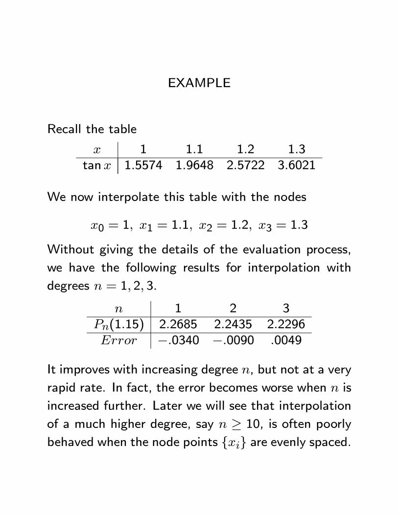
EXAMPLE
Recall the table
x 1 1.1 1.2 1.3tanx 1.5574 1.9648 2.5722 3.6021
We now interpolate this table with the nodes
x0 = 1, x1 = 1.1, x2 = 1.2, x3 = 1.3
Without giving the details of the evaluation process,
we have the following results for interpolation with
degrees n = 1, 2, 3.
n 1 2 3Pn(1.15) 2.2685 2.2435 2.2296Error −.0340 −.0090 .0049
It improves with increasing degree n, but not at a very
rapid rate. In fact, the error becomes worse when n is
increased further. Later we will see that interpolation
of a much higher degree, say n ≥ 10, is often poorly
behaved when the node points {xi} are evenly spaced.
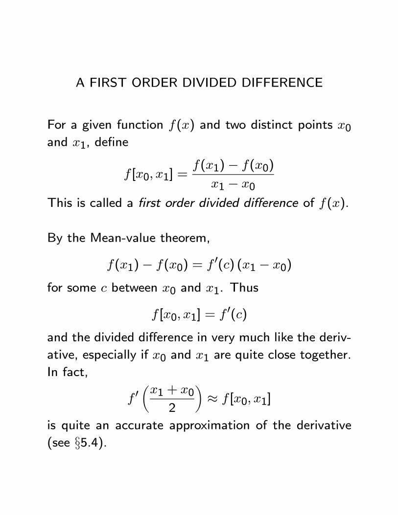
A FIRST ORDER DIVIDED DIFFERENCE
For a given function f(x) and two distinct points x0and x1, define
f [x0, x1] =f(x1)− f(x0)
x1 − x0
This is called a first order divided difference of f(x).
By the Mean-value theorem,
f(x1)− f(x0) = f 0(c) (x1 − x0)
for some c between x0 and x1. Thus
f [x0, x1] = f 0(c)and the divided difference in very much like the deriv-
ative, especially if x0 and x1 are quite close together.
In fact,
f 0µx1 + x02
¶≈ f [x0, x1]
is quite an accurate approximation of the derivative
(see §5.4).
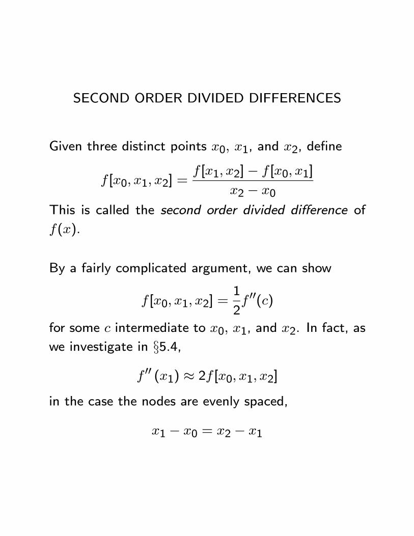
SECOND ORDER DIVIDED DIFFERENCES
Given three distinct points x0, x1, and x2, define
f [x0, x1, x2] =f [x1, x2]− f [x0, x1]
x2 − x0
This is called the second order divided difference of
f(x).
By a fairly complicated argument, we can show
f [x0, x1, x2] =1
2f 00(c)
for some c intermediate to x0, x1, and x2. In fact, as
we investigate in §5.4,f 00 (x1) ≈ 2f [x0, x1, x2]
in the case the nodes are evenly spaced,
x1 − x0 = x2 − x1
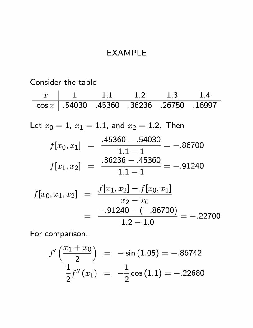
EXAMPLE
Consider the table
x 1 1.1 1.2 1.3 1.4cosx .54030 .45360 .36236 .26750 .16997
Let x0 = 1, x1 = 1.1, and x2 = 1.2. Then
f [x0, x1] =.45360− .54030
1.1− 1 = −.86700
f [x1, x2] =.36236− .45360
1.1− 1 = −.91240
f [x0, x1, x2] =f [x1, x2]− f [x0, x1]
x2 − x0
=−.91240− (−.86700)
1.2− 1.0 = −.22700For comparison,
f 0µx1 + x02
¶= − sin (1.05) = −.86742
1
2f 00 (x1) = −1
2cos (1.1) = −.22680
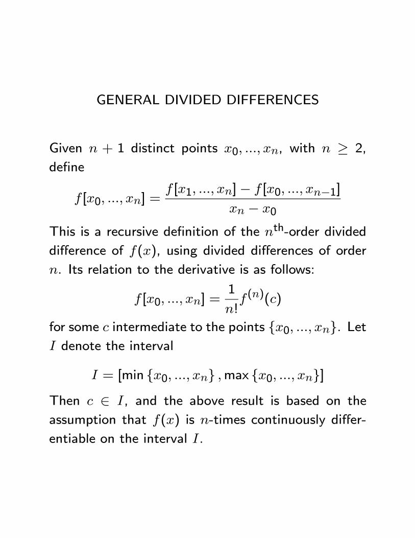
GENERAL DIVIDED DIFFERENCES
Given n + 1 distinct points x0, ..., xn, with n ≥ 2,
define
f [x0, ..., xn] =f [x1, ..., xn]− f [x0, ..., xn−1]
xn − x0
This is a recursive definition of the nth-order divided
difference of f(x), using divided differences of order
n. Its relation to the derivative is as follows:
f [x0, ..., xn] =1
n!f (n)(c)
for some c intermediate to the points {x0, ..., xn}. LetI denote the interval
I = [min {x0, ..., xn} ,max {x0, ..., xn}]Then c ∈ I, and the above result is based on the
assumption that f(x) is n-times continuously differ-
entiable on the interval I.
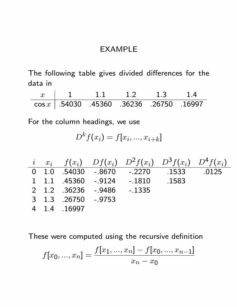
EXAMPLE
The following table gives divided differences for the
data in
x 1 1.1 1.2 1.3 1.4cosx .54030 .45360 .36236 .26750 .16997
For the column headings, we use
Dkf(xi) = f [xi, ..., xi+k]
i xi f(xi) Df(xi) D2f(xi) D3f(xi) D4f(xi)0 1.0 .54030 -.8670 -.2270 .1533 .01251 1.1 .45360 -.9124 -.1810 .15832 1.2 .36236 -.9486 -.13353 1.3 .26750 -.97534 1.4 .16997
These were computed using the recursive definition
f [x0, ..., xn] =f [x1, ..., xn]− f [x0, ..., xn−1]
xn − x0
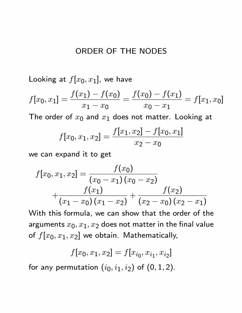
ORDER OF THE NODES
Looking at f [x0, x1], we have
f [x0, x1] =f(x1)− f(x0)
x1 − x0=
f(x0)− f(x1)
x0 − x1= f [x1, x0]
The order of x0 and x1 does not matter. Looking at
f [x0, x1, x2] =f [x1, x2]− f [x0, x1]
x2 − x0
we can expand it to get
f [x0, x1, x2] =f(x0)
(x0 − x1) (x0 − x2)
+f(x1)
(x1 − x0) (x1 − x2)+
f(x2)
(x2 − x0) (x2 − x1)
With this formula, we can show that the order of the
arguments x0, x1, x2 does not matter in the final value
of f [x0, x1, x2] we obtain. Mathematically,
f [x0, x1, x2] = f [xi0, xi1, xi2]
for any permutation (i0, i1, i2) of (0, 1, 2).
We can show in general that the value of f [x0, ..., xn]
is independent of the order of the arguments {x0, ..., xn},even though the intermediate steps in its calculations
using
f [x0, ..., xn] =f [x1, ..., xn]− f [x0, ..., xn−1]
xn − x0
are order dependent.
We can show
f [x0, ..., xn] = f [xi0, ..., xin]
for any permutation (i0, i1, ..., in) of (0, 1, ..., n).
COINCIDENT NODES
What happens when some of the nodes {x0, ..., xn}are not distinct. Begin by investigating what happens
when they all come together as a single point x0.
For first order divided differences, we have
limx1→x0
f [x0, x1] = limx1→x0
f(x1)− f(x0)
x1 − x0= f 0(x0)
We extend the definition of f [x0, x1] to coincident
nodes using
f [x0, x0] = f 0(x0)
For second order divided differences, recall
f [x0, x1, x2] =1
2f 00(c)
with c intermediate to x0, x1, and x2.
Then as x1 → x0 and x2 → x0, we must also have
that c→ x0. Therefore,
limx1→x0x2→x0
f [x0, x1, x2] =1
2f 00(x0)
We therefore define
f [x0, x0, x0] =1
2f 00(x0)
For the case of general f [x0, ..., xn], recall that
f [x0, ..., xn] =1
n!f (n)(c)
for some c intermediate to {x0, ..., xn}. Then
lim{x1,...,xn}→x0
f [x0, ..., xn] =1
n!f (n)(x0)
and we define
f [x0, ..., x0| {z }]n+1 times
=1
n!f (n)(x0)
What do we do when only some of the nodes are
coincident. This too can be dealt with, although we
do so here only by examples.
f [x0, x1, x1] =f [x1, x1]− f [x0, x1]
x1 − x0
=f 0(x1)− f [x0, x1]
x1 − x0The recursion formula can be used in general in this
way to allow all possible combinations of possibly co-
incident nodes.
LAGRANGE’S FORMULA FOR
THE INTERPOLATION POLYNOMIAL
Recall the general interpolation problem: find a poly-
nomial Pn(x) for which
deg(Pn) ≤ nPn(xi) = yi, i = 0, 1, · · · , n
with given data points
(x0, y0) , (x1, y1) , · · · , (xn, yn)and with {x0, ..., xn} distinct points.
In §5.1, we gave the solution as Lagrange’s formulaPn(x) = y0L0(x) + y1L1(x) + · · ·+ ynLn(x)
with {L0(x), ..., Ln(x)} the Lagrange basis polynomi-als. Each Lj is of degree n and it satisfies
Lj(xi) =
(1, j = i0, j 6= i
for i = 0, 1, ..., n.
THE NEWTON DIVIDED DIFFERENCE FORM
OF THE INTERPOLATION POLYNOMIAL
Let the data values for the problem
deg(Pn) ≤ nPn(xi) = yi, i = 0, 1, · · · , n
be generated from a function f(x):
yi = f(xi), i = 0, 1, ..., n
Using the divided differences
f [x0, x1], f [x0, x1, x2], ..., f [x0, ..., xn]
we can write the interpolation polynomials
P1(x), P2(x), ..., Pn(x)
in a way that is simple to compute.
P1(x) = f(x0) + f [x0, x1] (x− x0)P2(x) = f(x0) + f [x0, x1] (x− x0)
+f [x0, x1, x2] (x− x0) (x− x1)= P1(x) + f [x0, x1, x2] (x− x0) (x− x1)
For the case of the general problem
deg(Pn) ≤ nPn(xi) = yi, i = 0, 1, · · · , n
we have
Pn(x) = f(x0) + f [x0, x1] (x− x0)+f [x0, x1, x2] (x− x0) (x− x1)+f [x0, x1, x2, x3] (x− x0) (x− x1) (x− x2)+ · · ·+f [x0, ..., xn] (x− x0) · · · (x− xn−1)
From this we have the recursion relation
Pn(x) = Pn−1(x)+f [x0, ..., xn] (x− x0) · · · (x− xn−1)
in which Pn−1(x) interpolates f(x) at the points in{x0, ..., xn−1}.

Example: Recall the table
i xi f(xi) Df(xi) D2f(xi) D3f(xi) D4f(xi)0 1.0 .54030 -.8670 -.2270 .1533 .01251 1.1 .45360 -.9124 -.1810 .15832 1.2 .36236 -.9486 -.13353 1.3 .26750 -.97534 1.4 .16997
withDkf(xi) = f [xi, ..., xi+k], k = 1, 2, 3, 4. Then
P1(x) = .5403− .8670 (x− 1)P2(x) = P1(x)− .2270 (x− 1) (x− 1.1)P3(x) = P2(x) + .1533 (x− 1) (x− 1.1) (x− 1.2)P4(x) = P3(x)
+.0125 (x− 1) (x− 1.1) (x− 1.2) (x− 1.3)Using this table and these formulas, we have the fol-
lowing table of interpolants for the value x = 1.05.
The true value is cos(1.05) = .49757105.
n 1 2 3 4Pn(1.05) .49695 .49752 .49758 .49757Error 6.20E−4 5.00E−5 −1.00E−5 0.0
EVALUATION OF THE DIVIDED DIFFERENCE
INTERPOLATION POLYNOMIAL
Let
d1 = f [x0, x1]d2 = f [x0, x1, x2]
...dn = f [x0, ..., xn]
Then the formula
Pn(x) = f(x0) + f [x0, x1] (x− x0)+f [x0, x1, x2] (x− x0) (x− x1)+f [x0, x1, x2, x3] (x− x0) (x− x1) (x− x2)+ · · ·+f [x0, ..., xn] (x− x0) · · · (x− xn−1)
can be written as
Pn(x) = f(x0) + (x− x0) (d1 + (x− x1) (d2 + · · ·+(x− xn−2) (dn−1 + (x− xn−1) dn) · · · )
Thus we have a nested polynomial evaluation, and
this is quite efficient in computational cost.
Top Related