≈≈≈≈≈≈≈≈≈≈≈≈≈≈≈≈≈≈≈≈≈ HYPOTHESIS TESTING ≈≈≈≈≈≈≈≈≈≈≈≈≈≈≈≈≈≈≈≈≈

1

HYPOTHESIS TESTING Documents prepared for use in course B01.1305, New York University, Stern School of Business

The logic of hypothesis testing, as compared to jury trials page 3 This simple layout shows an excellent correspondence between hypothesis testing and jury decision-making.

t test examples page 4

Here are some examples of the very widely used t test. The t test through Minitab page 8

This shows an example of a two-sample problem, as performed by Minitab.

One-sided tests page 13

We need to be very careful in using one-sided tests. Here are some serious thoughts and some tough examples.

An example of a one-sided testing environment page 18

Most of the time we prefer two-sided tests, but there are some clear situations calling for one-sided investigations.

Comparing the means of two groups page 19

The two-sample t test presents some confusion because of the uncertainty about whether or not to assume equal standard deviations.

Comparing two groups with Minitab 14 page 24

Minitab 14 reduces all the confusion of the previous section down to a few simple choices.

≈≈≈≈≈≈≈≈≈≈≈≈≈≈≈≈≈≈≈≈≈ HYPOTHESIS TESTING ≈≈≈≈≈≈≈≈≈≈≈≈≈≈≈≈≈≈≈≈≈

2

Does it matter which form of the two-sample t test we use? page 28

There is a lot of confusion about which form of the two-sample test should be used. But does it really matter?

Summary of hypothesis tests page 30

This gives, in chart form, a layout of the commonly-used statistical hypothesis tests.

What are the uses for hypothesis tests? page 33

This discusses the situations in which we use hypothesis testing. Included also is a serious discussion of error rates and power curves.

© Gary Simon, 2007

Cover photo: Yasgur farm, Woodstock, New York revision date 16 APR 2007

||||| HYPOTHESIS TESTING COMPARED TO JURY TRIALS|||||

3

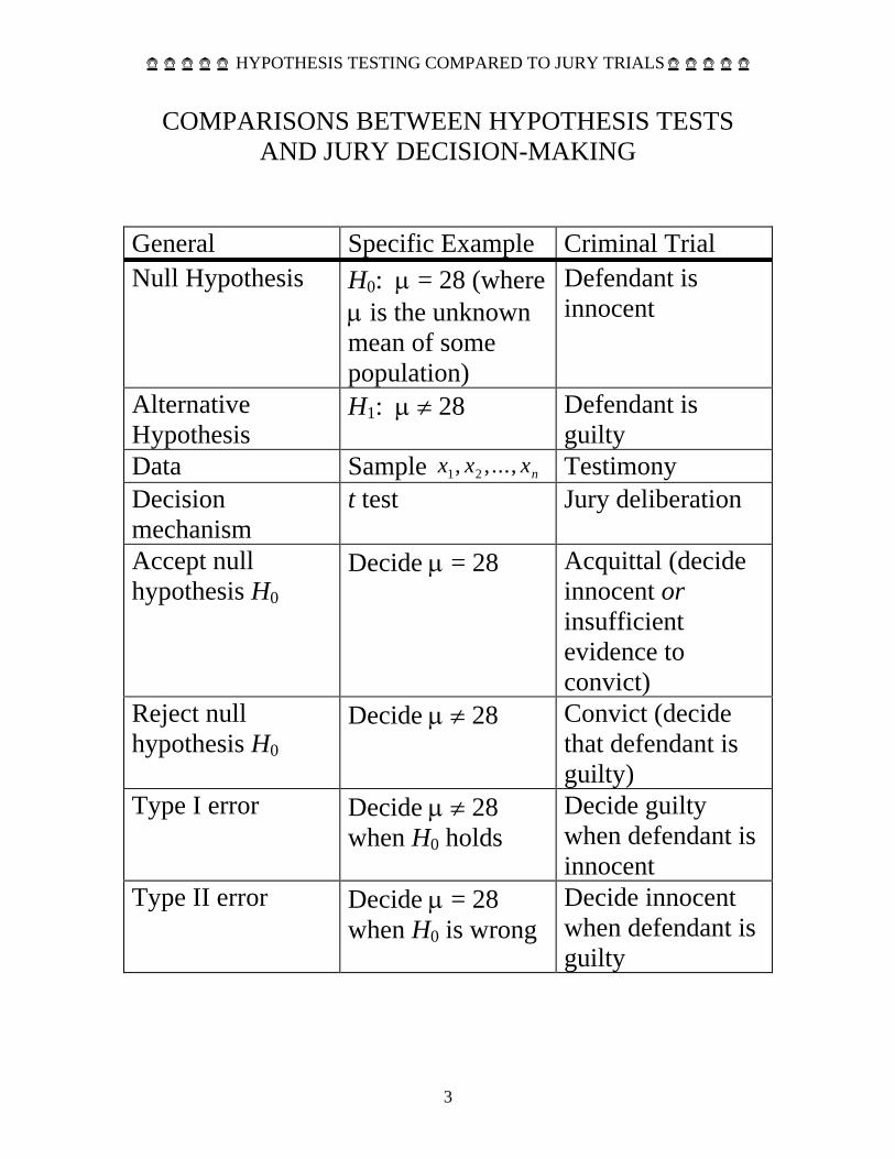
COMPARISONS BETWEEN HYPOTHESIS TESTS AND JURY DECISION-MAKING

General Specific Example Criminal Trial Null Hypothesis H0: μ = 28 (where

μ is the unknown mean of some population)

Defendant is innocent

Alternative Hypothesis

H1: μ ≠ 28 Defendant is guilty

Data Sample x x xn1 2, , ..., Testimony Decision mechanism

t test Jury deliberation

Accept null hypothesis H0

Decide μ = 28 Acquittal (decide innocent or insufficient evidence to convict)

Reject null hypothesis H0

Decide μ ≠ 28 Convict (decide that defendant is guilty)

Type I error Decide μ ≠ 28 when H0 holds

Decide guilty when defendant is innocent

Type II error Decide μ = 28 when H0 is wrong

Decide innocent when defendant is guilty

¢¢¢¢¢¢¢¢¢¢ t TEST EXAMPLES ¢¢¢¢¢¢¢¢¢¢

4

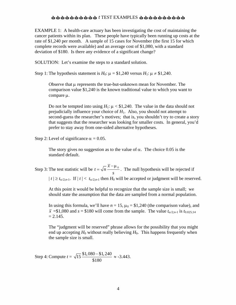
EXAMPLE 1: A health-care actuary has been investigating the cost of maintaining the cancer patients within its plan. These people have typically been running up costs at the rate of $1,240 per month. A sample of 15 cases for November (the first 15 for which complete records were available) and an average cost of $1,080, with a standard deviation of $180. Is there any evidence of a significant change? SOLUTION: Let’s examine the steps to a standard solution. Step 1: The hypothesis statement is H0: μ = $1,240 versus H1: μ ≠ $1,240.

Observe that μ represents the true-but-unknown mean for November. The comparison value $1,240 is the known traditional value to which you want to compare μ. Do not be tempted into using H1: μ < $1,240. The value in the data should not prejudicially influence your choice of H1. Also, you should not attempt to second-guess the researcher’s motives; that is, you shouldn’t try to create a story that suggests that the researcher was looking for smaller costs. In general, you’d prefer to stay away from one-sided alternative hypotheses.

Step 2: Level of significance α = 0.05.

The story gives no suggestion as to the value of α. The choice 0.05 is the standard default.

Step 3: The test statistic will be 0xt n

s−μ

= . The null hypothesis will be rejected if

| t | ≥ tα/2;n-1. If | t | < tα/2;n-1 then H0 will be accepted or judgment will be reserved.

At this point it would be helpful to recognize that the sample size is small; we should state the assumption that the data are sampled from a normal population. In using this formula, we’ll have n = 15, μ0 = $1,240 (the comparison value), and x =$1,080 and s = $180 will come from the sample. The value tα/2;n-1 is t0.025;14 = 2.145. The “judgment will be reserved” phrase allows for the possibility that you might end up accepting H0 without really believing H0. This happens frequently when the sample size is small.

Step 4: Compute t = $1,080 $1, 24015$180− ≈ -3.443.

¢¢¢¢¢¢¢¢¢¢ t TEST EXAMPLES ¢¢¢¢¢¢¢¢¢¢

5

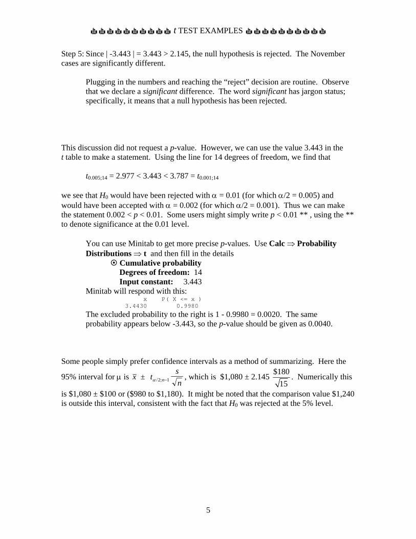
Step 5: Since | -3.443 | = 3.443 > 2.145, the null hypothesis is rejected. The November cases are significantly different.

Plugging in the numbers and reaching the “reject” decision are routine. Observe that we declare a significant difference. The word significant has jargon status; specifically, it means that a null hypothesis has been rejected.

This discussion did not request a p-value. However, we can use the value 3.443 in the t table to make a statement. Using the line for 14 degrees of freedom, we find that

t0.005;14 = 2.977 < 3.443 < 3.787 = t0.001;14 we see that H0 would have been rejected with α = 0.01 (for which α/2 = 0.005) and would have been accepted with α = 0.002 (for which α/2 = 0.001). Thus we can make the statement 0.002 < p < 0.01. Some users might simply write p < 0.01 ** , using the ** to denote significance at the 0.01 level.

You can use Minitab to get more precise p-values. Use Calc ⇒ Probability Distributions ⇒ t and then fill in the details

Cumulative probability Degrees of freedom: 14 Input constant: 3.443

Minitab will respond with this: x P( X <= x ) 3.4430 0.9980

The excluded probability to the right is 1 - 0.9980 = 0.0020. The same probability appears below -3.443, so the p-value should be given as 0.0040.

Some people simply prefer confidence intervals as a method of summarizing. Here the

95% interval for μ is x ± tsnnα / ;2 1− , which is $1,080 ± 2.145 $180

15. Numerically this

is $1,080 ± $100 or ($980 to $1,180). It might be noted that the comparison value $1,240 is outside this interval, consistent with the fact that H0 was rejected at the 5% level.

¢¢¢¢¢¢¢¢¢¢ t TEST EXAMPLES ¢¢¢¢¢¢¢¢¢¢

6

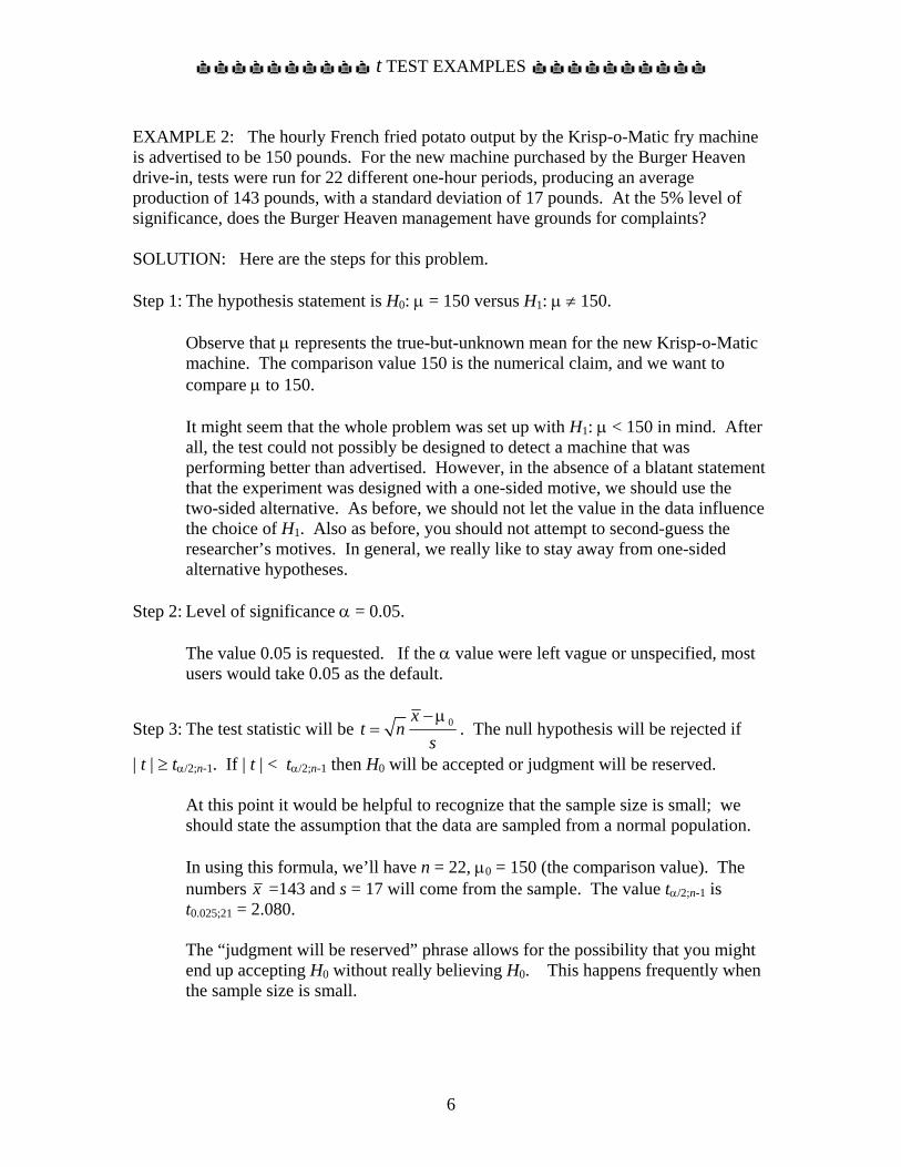
EXAMPLE 2: The hourly French fried potato output by the Krisp-o-Matic fry machine is advertised to be 150 pounds. For the new machine purchased by the Burger Heaven drive-in, tests were run for 22 different one-hour periods, producing an average production of 143 pounds, with a standard deviation of 17 pounds. At the 5% level of significance, does the Burger Heaven management have grounds for complaints? SOLUTION: Here are the steps for this problem. Step 1: The hypothesis statement is H0: μ = 150 versus H1: μ ≠ 150.

Observe that μ represents the true-but-unknown mean for the new Krisp-o-Matic machine. The comparison value 150 is the numerical claim, and we want to compare μ to 150. It might seem that the whole problem was set up with H1: μ < 150 in mind. After all, the test could not possibly be designed to detect a machine that was performing better than advertised. However, in the absence of a blatant statement that the experiment was designed with a one-sided motive, we should use the two-sided alternative. As before, we should not let the value in the data influence the choice of H1. Also as before, you should not attempt to second-guess the researcher’s motives. In general, we really like to stay away from one-sided alternative hypotheses.

Step 2: Level of significance α = 0.05.

The value 0.05 is requested. If the α value were left vague or unspecified, most users would take 0.05 as the default.

Step 3: The test statistic will be 0xt n

s−μ

= . The null hypothesis will be rejected if

| t | ≥ tα/2;n-1. If | t | < tα/2;n-1 then H0 will be accepted or judgment will be reserved.

At this point it would be helpful to recognize that the sample size is small; we should state the assumption that the data are sampled from a normal population. In using this formula, we’ll have n = 22, μ0 = 150 (the comparison value). The numbers x =143 and s = 17 will come from the sample. The value tα/2;n-1 is t0.025;21 = 2.080. The “judgment will be reserved” phrase allows for the possibility that you might end up accepting H0 without really believing H0. This happens frequently when the sample size is small.

¢¢¢¢¢¢¢¢¢¢ t TEST EXAMPLES ¢¢¢¢¢¢¢¢¢¢

7

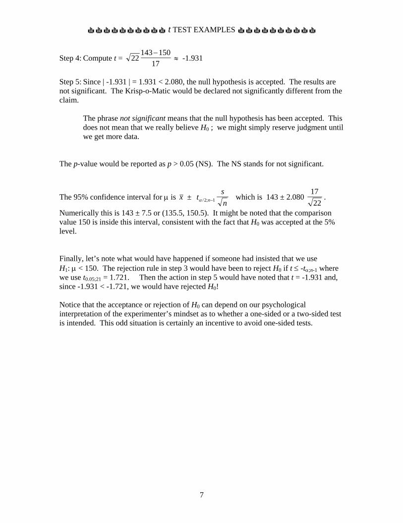
Step 4: Compute t = 22143 150

17−

≈ -1.931

Step 5: Since | -1.931 | = 1.931 < 2.080, the null hypothesis is accepted. The results are not significant. The Krisp-o-Matic would be declared not significantly different from the claim.

The phrase not significant means that the null hypothesis has been accepted. This does not mean that we really believe H0 ; we might simply reserve judgment until we get more data.

The p-value would be reported as p > 0.05 (NS). The NS stands for not significant.

The 95% confidence interval for μ is x ± tsnnα / ;2 1− which is 143 ± 2.080

1722

.

Numerically this is 143 ± 7.5 or (135.5, 150.5). It might be noted that the comparison value 150 is inside this interval, consistent with the fact that H0 was accepted at the 5% level. Finally, let’s note what would have happened if someone had insisted that we use H1: μ < 150. The rejection rule in step 3 would have been to reject H0 if t ≤ -tα;n-1 where we use t0.05;21 = 1.721. Then the action in step 5 would have noted that t = -1.931 and, since -1.931 < -1.721, we would have rejected H0! Notice that the acceptance or rejection of H0 can depend on our psychological interpretation of the experimenter’s mindset as to whether a one-sided or a two-sided test is intended. This odd situation is certainly an incentive to avoid one-sided tests.

ƒƒƒƒƒƒƒƒ THE t TEST THROUGH MINITAB ƒƒƒƒƒƒƒƒ

8

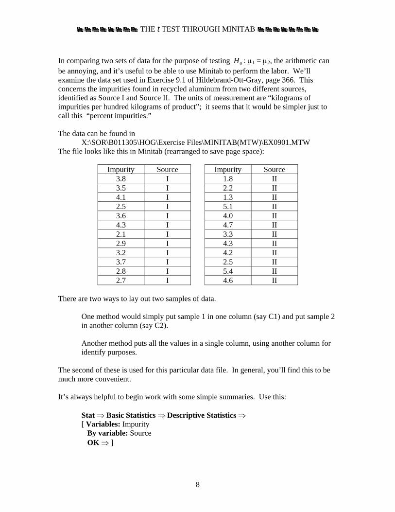
In comparing two sets of data for the purpose of testing H0 : μ1 = μ2, the arithmetic can be annoying, and it’s useful to be able to use Minitab to perform the labor. We’ll examine the data set used in Exercise 9.1 of Hildebrand-Ott-Gray, page 366. This concerns the impurities found in recycled aluminum from two different sources, identified as Source I and Source II. The units of measurement are “kilograms of impurities per hundred kilograms of product”; it seems that it would be simpler just to call this “percent impurities.” The data can be found in

X:\SOR\B011305\HOG\Exercise Files\MINITAB(MTW)\EX0901.MTW The file looks like this in Minitab (rearranged to save page space):

Impurity Source Impurity Source 3.8 I 1.8 II 3.5 I 2.2 II 4.1 I 1.3 II 2.5 I 5.1 II 3.6 I 4.0 II 4.3 I 4.7 II 2.1 I 3.3 II 2.9 I 4.3 II 3.2 I 4.2 II 3.7 I 2.5 II 2.8 I 5.4 II 2.7 I 4.6 II

There are two ways to lay out two samples of data.

One method would simply put sample 1 in one column (say C1) and put sample 2 in another column (say C2). Another method puts all the values in a single column, using another column for identify purposes.

The second of these is used for this particular data file. In general, you’ll find this to be much more convenient. It’s always helpful to begin work with some simple summaries. Use this:

Stat ⇒ Basic Statistics ⇒ Descriptive Statistics ⇒ [ Variables: Impurity By variable: Source OK ⇒ ]

ƒƒƒƒƒƒƒƒ THE t TEST THROUGH MINITAB ƒƒƒƒƒƒƒƒ

9

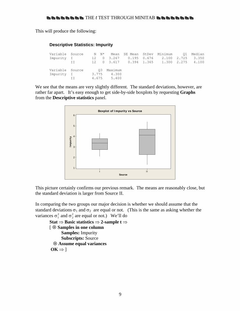
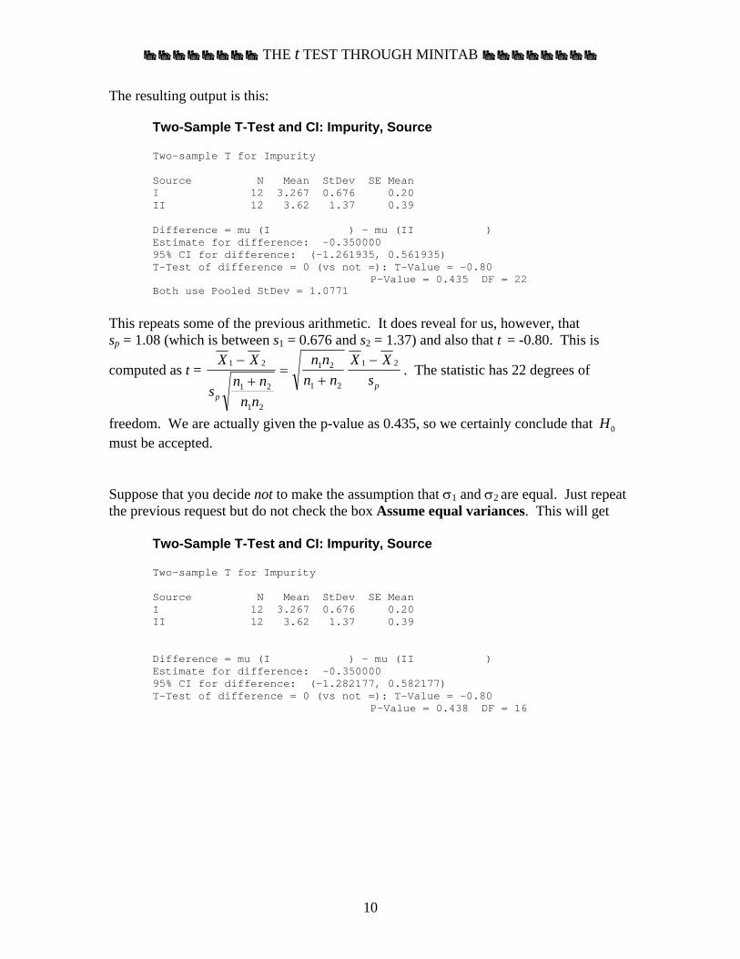
This will produce the following:

Descriptive Statistics: Impurity Variable Source N N* Mean SE Mean StDev Minimum Q1 Median Impurity I 12 0 3.267 0.195 0.676 2.100 2.725 3.350 II 12 0 3.617 0.394 1.365 1.300 2.275 4.100 Variable Source Q3 Maximum Impurity I 3.775 4.300 II 4.675 5.400

We see that the means are very slightly different. The standard deviations, however, are rather far apart. It’s easy enough to get side-by-side boxplots by requesting Graphs from the Descriptive statistics panel.

Source

Impu

rity

III

6

5

4

3

2

1

Boxplot of Impurity vs Source

This picture certainly confirms our previous remark. The means are reasonably close, but the standard deviation is larger from Source II. In comparing the two groups our major decision is whether we should assume that the standard deviations σ1 and σ2 are equal or not. (This is the same as asking whether the variances σ1

2 and σ22 are equal or not.) We’ll do

Stat ⇒ Basic statistics ⇒ 2-sample t ⇒ [ Samples in one column Samples: Impurity Subscripts: Source Assume equal variances OK ⇒ ]

ƒƒƒƒƒƒƒƒ THE t TEST THROUGH MINITAB ƒƒƒƒƒƒƒƒ

10

This repeats some of the previous arithmetic. It does reveal for us, however, that sp = 1.08 (which is between s1 = 0.676 and s2 = 1.37) and also that t = -0.80. This is

computed as t = X X

sn n

n n

n nn n

X Xs

pp

1 2

1 2

1 2

1 2

1 2

1 2−+

=+

−. The statistic has 22 degrees of

freedom. We are actually given the p-value as 0.435, so we certainly conclude that H0 must be accepted. Suppose that you decide not to make the assumption that σ1 and σ2 are equal. Just repeat the previous request but do not check the box Assume equal variances. This will get

Two-Sample T-Test and CI: Impurity, Source Two-sample T for Impurity Source N Mean StDev SE Mean I 12 3.267 0.676 0.20 II 12 3.62 1.37 0.39 Difference = mu (I ) - mu (II ) Estimate for difference: -0.350000 95% CI for difference: (-1.282177, 0.582177) T-Test of difference = 0 (vs not =): T-Value = -0.80

P-Value = 0.438 DF = 16

The resulting output is this: Two-Sample T-Test and CI: Impurity, Source Two-sample T for Impurity Source N Mean StDev SE Mean I 12 3.267 0.676 0.20 II 12 3.62 1.37 0.39 Difference = mu (I ) - mu (II ) Estimate for difference: -0.350000 95% CI for difference: (-1.261935, 0.561935) T-Test of difference = 0 (vs not =): T-Value = -0.80

P-Value = 0.435 DF = 22 Both use Pooled StDev = 1.0771

ƒƒƒƒƒƒƒƒ THE t TEST THROUGH MINITAB ƒƒƒƒƒƒƒƒ

11

The test statistic is computed as t = X Xsn

sn

1 2

12

1

22

2

−

+

, with the degrees of freedom computed as

n n

n

sn

sn

sn

n

sn

sn

sn

1 2

2

12

1

12

1

22

2

2

1

22

2

12

1

22

2

2

1 1

1 1

− −

−+

F

H

GGGG

I

K

JJJJ+ −

+

F

H

GGGG

I

K

JJJJ

b gb g

b g b g

, which Minitab truncates to the

previous integer, here 16. While this procedure is elaborate, and while there is rather persuasive evidence that σ1 ≠ σ2, the values produced by t are nearly identical (rounded to -0.80 for both) and the p-values are nearly identical (0.435 and 0.438). You might wonder about a test for H0 : σ1 = σ2 versus H1 : σ1 ≠ σ2. (We’re now using the symbols H0 and H1 to refer to the hypotheses about the standard deviations.) Such a test is actually available through the commands

Stat ⇒ ANOVA ⇒ Test for Equal Variances ⇒ [ Response: Impurity Factors: Source OK ⇒ ]

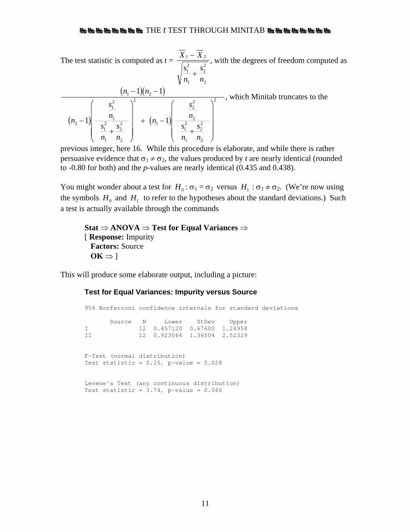
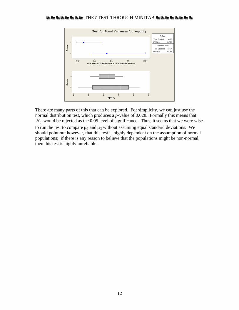
This will produce some elaborate output, including a picture:

Test for Equal Variances: Impurity versus Source 95% Bonferroni confidence intervals for standard deviations Source N Lower StDev Upper I 12 0.457120 0.67600 1.24958 II 12 0.923064 1.36504 2.52329 F-Test (normal distribution) Test statistic = 0.25, p-value = 0.028 Levene's Test (any continuous distribution) Test statistic = 3.74, p-value = 0.066

ƒƒƒƒƒƒƒƒ THE t TEST THROUGH MINITAB ƒƒƒƒƒƒƒƒ

12

Sour

ce

95% Bonferroni Confidence Intervals for StDevs

II

I

2.52.01.51.00.5

Sour

ce

Impurity

II

I

654321

F-Test

0.066

Test Statistic 0.25P-Value 0.028

Levene's Test

Test Statistic 3.74P-Value

Test for Equal Variances for Impurity

There are many parts of this that can be explored. For simplicity, we can just use the normal distribution test, which produces a p-value of 0.028. Formally this means that H0 would be rejected as the 0.05 level of significance. Thus, it seems that we were wise to run the test to compare μ1 and μ2 without assuming equal standard deviations. We should point out however, that this test is highly dependent on the assumption of normal populations; if there is any reason to believe that the populations might be non-normal, then this test is highly unreliable.

‰‰‰‰‰‰‰‰‰‰ ONE SIDED TESTS ‰‰‰‰‰‰‰‰‰‰

13

In some cases, only one side of μ0 is interesting. For instance, results suggesting that really μ > μ0 might be valuable while results suggesting that μ < μ0 might be worthless. The formulation of the hypotheses is H0: μ = μ0 versus H1: μ > μ0.

This problem is written equivalently as H0: μ ≤ μ0 versus H1: μ > μ0. The procedure now is to reject if t ≥ tα;n-1. For instance, if n = 20 and α = 0.05, then you reject H0 when t ≥ 1.729. Observe that no rejection of H0 occurs for negative t; even t = -500 would not cause rejection of H0. Below is a parallel version of these statements for problems organized so that values below μ0 are interesting.

≈≈≈≈≈≈≈≈≈≈≈≈≈≈≈≈≈≈≈≈≈≈≈≈≈≈≈≈≈≈≈≈≈≈≈≈≈≈≈≈≈≈≈≈≈≈≈≈≈≈≈≈≈≈≈≈≈≈≈≈ For instance, results suggesting that really μ < μ0 might be valuable while results suggesting that μ > μ0 might be worthless. The formulation of the hypotheses is H0: μ = μ0 versus H1: μ < μ0.

This problem is written equivalently as H0: μ ≥ μ0 versus H1: μ < μ0. The procedure now is to reject if t ≤ -tα;n-1. For instance, if n = 20 and α = 0.05, then you reject H0 when t ≤ -1.729. Observe that no rejection of H0 occurs for positive t; even t = 500 would not cause rejection of H0. ≈≈≈≈≈≈≈≈≈≈≈≈≈≈≈≈≈≈≈≈≈≈≈≈≈≈≈≈≈≈≈≈≈≈≈≈≈≈≈≈≈≈≈≈≈≈≈≈≈≈≈≈≈≈≈≈≈≈≈≈

It is valuable to note that one-tail tests make it easier to reject H0 , at least when x is on the interesting side of μ0. For instance if n = 20, α = 0.05, μ0 = 1,200, x = 1,260, s = 142,

then t = 201 260 1 200

142, ,−

≈ 1.89.

If the problem is H0: μ = 1,200 versus H1: μ ≠ 1,200, then the procedure is to reject if t ≥ 2.093. This would cause H0 to be accepted.

If the problem is H0: μ = 1,200 versus H1: μ > 1,200, then the procedure is to reject if t ≥ 1.729. This would cause H0 to be rejected.

Your motives will be questioned whenever you do a one-tail test. GOOD ADVICE: Always use two-sided tests, except for those cases which are clearly and blatantly one-sided from their description.

‰‰‰‰‰‰‰‰‰‰ ONE SIDED TESTS ‰‰‰‰‰‰‰‰‰‰

14

If you find yourself looking at the data to decide the form of H1, then you should be doing a two-tail test. The following situations are examples in which one-tail tests are definitely appropriate:

(a) Investigating legal limits in situations for which only results on one side of a stated limit mean trouble. These include problems on pollution allowances.

(b) Performing an audit in which only one side (undervaluing, say) is relevant.

If can sometimes be argued that one-sided tests should be used for these cases: (c) Comparing a new product to a standard product. (d) Investigating advertising claims or sales pitches about the merits of a

product. Virtually all other tests should be done two-sided. Particular cases to watch out for:

(e) Comparing two products, both of which are already on the market. (f) Comparing two medical procedures. (g) t tests on regression coefficients. (h) Investigating scientific claims.

Special arguments can be invoked in almost every instance. If you have any doubts about whether you should be doing a one-tail test or a two-tail test.....then do a two-tail test. This document takes the broad point of view that every test should be done two-sided, with exceptions only for those situations like (a) or (b) or for those situations in which there is a tradition of one-sided tests. Please see the last paragraph for an interesting defense of one-sided tests. In dealing with hypothesis tests, there are rules about proper procedure. The prime concern is that a glance at the data influences the manner in which the test is conceived and conducted. Specifically....you must not inspect the data before you formulate H0 and H1. The concern is that you will decide whether this is a one-sided test or two-sided test after examining the data. Consider this interesting situation. The Chow City Supermarket chain has just installed Magiceye optical scanning equipment at the checkout counters of its Mayville store. After one month of experimentation, management notes that the Magiceye system gives a checkout rate of 6.45 items per minute. This is computed as the number of line items processed per minute of time that a checkout counter is open, and necessarily involves time for bagging groceries and processing coupons. The manager of the Mayville store asked to try System M, an alternate system, and a couple of checkout counters were equiped with System M. Over the next few days, using different clerks, System M was

‰‰‰‰‰‰‰‰‰‰ ONE SIDED TESTS ‰‰‰‰‰‰‰‰‰‰

15

evaluated for 50 separate one-hour periods. These 50 periods showed an average checkout rate of 6.61 items per minute, with a standard deviation of 0.62. What conclusions should be reached? At company headquarters, the problem was formulated as H0 : μ = 6.45 versus H1 : μ ≠ 6.45. (Here μ is the unknown mean for System M.) This was done as a two-sided problem because management expressed an interest in either side of 6.45. If System M does significantly worse, then the large purchase of Magiceye has been justified. If System M does significantly better, then additional installations might use

System M. The test statistic was computed as t = 506 61 6 45

0 62. .

.−

≈ 1.825.

The comparison point, using the 5% level of significance, is 2.011.

This is the value t0.025;49. This was obtained by quick interpolation between t0.025;40 = 2.021 and t0.025;60 = 2.000. If your t table lacks entries beyond 30 df, then use t0.025;∞ = 1.96.

Since the t statistic is between -2.011 and +2.011, the null hypothesis is accepted. The conclusion is that there is no significant difference between Magiceye and System M. The results were transmitted back to the manager of the Mayville store. He insisted that he wanted to test System M only because it would be an improvement. After all, why would he be interested in a system no better than what he already has? He redid the analysis. The problem was formulated as H0 : μ = 6.45 versus alternative H1 : μ > 6.45. This was done as a one-sided problem because the Mayville manager expected to show that

System M was superior. The test statistic was computed as t = 506 61 6 45

0 62. .

.−

≈ 1.825.

The comparison point, using the 5% level of significance, is 1.678.

This is the value t0.05;49, obtained by quick interpolation between t0.05;40 = 1.684 and t0.05;60 = 1.671. If your t table lacks entries beyond 30 df, then you must use t0.05;∞ = 1.645.

Since the value of t exceeds 1.678, the null hypothesis is rejected. The conclusion is that System M is significantly faster than Magiceye. This example illustrates why many statisticians, especially those at regulatory agencies, are very wary of one-sided tests.

‰‰‰‰‰‰‰‰‰‰ ONE SIDED TESTS ‰‰‰‰‰‰‰‰‰‰

16

Now consider this example. The Ultra! soft drink company has retooled the chemical filtration step through which its cola drink is passed, in the expectation that the caffeine concentration will be reduced. The target concentration is 125 mg per twelve-ounce can, the current content of its UltraCola drink. The new method is used to produce 96 cans, and the caffeine concentration of each can is measured. The resulting 96 values have a mean concentration of 125.81 mg and a standard deviation of 4.2 mg. The problem was formulated as a test of H0 : μ = 125 versus H1 : μ ≠ 125, using μ to represent the true-but-unknown concentration using the retooled filtration step. The t

statistic was computed as t = 9612581 125

4 2.

.−

≈ 1.890.

The comparison point, using the 5% level of significance, is t0.025;95 = is 1.992.

This was obtained by crude interpolation between t0.025;60 = 2.000 and t0.025;120 = 1.980. If your t table does not have lines past 30 df, use t0.025;∞ = 1.96.

Since the computed value of t, namely 1.890, is between -1.992 and +1.992, the null hypothesis must be accepted. One would conclude that this change has had no significant impact on the caffeine concentration. The analysis above was shown to a marketing specialist who refused to pass up a potentially interesting finding. He reinterpreted the situation as a desire to make a higher caffeine drink in order to tap into the “high-wired” market segment. Accordingly, using the same information, he rewrote the analysis as follows: The problem was formulated as a test of H0 : μ = 125 versus H1 : μ > 125, using μ to represent the true-but-unknown concentration using the retooled filtration step. The t

statistic was computed as t = 9612581 125

4 2.

.−

≈ 1.890.

The comparison point, using the 5% level of significance, is t0.05;95 = 1.663.

This was obtained by crude interpolation between t0.05;60 = 1.671 and t0.05;120 = 1.658. If your t table does not have lines past 30 df, use t0.05;∞ = 1.645.

Since the computed value of t, namely 1.890, exceeds 1.663 the null hypothesis must be rejected. One would conclude that this change has had a significant increasing impact on the caffeine concentration. The marketing specialist recommended that the product be developed under the name UltraVolt Cola. He may have ignored the fact that the typical soda drinker may not be able to distinguish 125 mg from (estimated) 125.81 mg.

‰‰‰‰‰‰‰‰‰‰ ONE SIDED TESTS ‰‰‰‰‰‰‰‰‰‰

17

Each of these examples illustrates that

A nonsignificant result can sometimes be made significant by revising the procedure to be one-sided. A peek at the data can be a powerful influence to the person formulating the hypotheses. We must specify H0 and H1 without a look at the data.

As a practical question, we have to ask what to do if we see the data before we have a chance to specify the hypotheses. After all, there are cases in which the data are presented to you before you have any chance to react! In such a situation, your only reasonable strategy is to try to imagine what you would have done if you understood the experimental layout but had not seen the data. This is tough. It is probably reasonable to recommend a two-sided test at the 5% level. You are almost certainly unable to honorably recommend a one-sided test.

There is an interesting defense of the one-sided methodology. Suppose that you want to compare a new medical procedure to an existing procedure. The experiment needs to be done on human subjects. Experimental protocols must be developed in terms of statistical power, and there must be calculations supporting the notion that the sample size n will be large enough to achieve desired power. The needed value of n will be smaller for a one-sided test, meaning that fewer subjects will be needed in the experiment. This means that the knowledge will be obtaining while putting fewer subjects through the inferior medical procedure! This is discussed in “The Ethics of Sample Size: Two-Sided Testing and One-Sided Thinking,” by J. André Knottnerus and Lex M. Bouter, Journal of Clinical Epidemiology, vol 54, #2, February 2001, pp 109-110.

‘‘‘‘‘EXAMPLE OF A ONE-SIDED TESTING ENVIRONMENT ‘‘‘‘‘

18

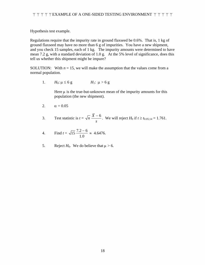
Hypothesis test example. Regulations require that the impurity rate in ground flaxseed be 0.6%. That is, 1 kg of ground flaxseed may have no more than 6 g of impurities. You have a new shipment, and you check 15 samples, each of 1 kg. The impurity amounts were determined to have mean 7.2 g, with a standard deviation of 1.0 g. At the 5% level of significance, does this tell us whether this shipment might be impure? SOLUTION: With n = 15, we will make the assumption that the values come from a normal population.

1. H0: μ ≤ 6 g H1: μ > 6 g

Here μ is the true-but-unknown mean of the impurity amounts for this population (the new shipment).

2. α = 0.05

3. Test statistic is t = 6Xns− . We will reject H0 if t ≥ t0.05;14 = 1.761.

4. Find t = 7.2 6151.0− ≈ 4.6476.

5. Reject H0. We do believe that μ > 6.

COMPARING THE MEANS OF TWO GROUPS

19

In comparing two samples of measured data, there are several possibilities for structuring a test. Population standard

deviations assumed equal; σA = σB

Population standard deviations σA and σB

allowed to be different Sample sizes nA and nB both large (30 or more)

Use t test with sp ; degrees of freedom is nA+nB-2 ; as degrees of freedom is large this is approximately normal (whether the populations are assumed normal or not).

Use statistic

B

B

A

A

BA

ns

ns

XX22

+

−

which will be approximately normal.

At least one of the sample sizes is small [must assume normal populations]

Use t test with sp ; degrees of freedom is nA+nB-2. Use statistic

X Xsn

sn

A B

A

A

B

B

−

+2 2

which will approximately be t with approximate degrees of freedom noted at end of this document.

It is strongly recommended that you invoke the assumption σA = σB unless the data are presenting very convincing evidence that these are unequal. As a quick approximation,

you can reasonably believe that σA = σB whenever 12

2≤ ≤ss

A

B

. If you think that

σA ≠ σB , then you should seriously consider whether you really want to ask whether μA = μB . Here are a number of illustrations of these calculations. Two brands of commercial frying fat are to be compared in terms of saturated fat content, and the standard of comparison is expressed in terms of grams of saturated fat per tablespoon. A whole tablespoon contains 20 grams of fat, but only some of that amount is saturated. Samples are obtained for brands A and B, resulting in the following:

Fat Number of Samples Average Standard Deviation A 40 6.02 0.86 B 50 6.41 0.90

Test whether or not the two fats have equal amounts of saturated fat. State your conclusion in terms of the p-value.

COMPARING THE MEANS OF TWO GROUPS

20

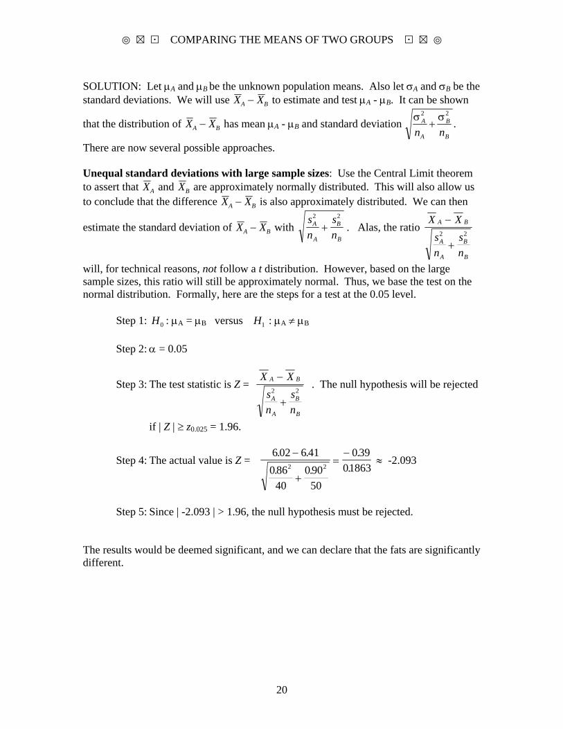
SOLUTION: Let μA and μB be the unknown population means. Also let σA and σB be the standard deviations. We will use X XA B− to estimate and test μA - μB. It can be shown

that the distribution of X XA B− has mean μA - μB and standard deviation σ σA

A

B

Bn n

2 2

+ .

There are now several possible approaches. Unequal standard deviations with large sample sizes: Use the Central Limit theorem to assert that XA and XB are approximately normally distributed. This will also allow us to conclude that the difference X XA B− is also approximately distributed. We can then

estimate the standard deviation of X XA B− with sn

sn

A

A

B

B

2 2

+ . Alas, the ratio X X

sn

sn

A B

A

A

B

B

−

+2 2

will, for technical reasons, not follow a t distribution. However, based on the large sample sizes, this ratio will still be approximately normal. Thus, we base the test on the normal distribution. Formally, here are the steps for a test at the 0.05 level.

Step 1: H0 : μA = μB versus H1 : μA ≠ μB Step 2: α = 0.05

Step 3: The test statistic is Z = X X

sn

sn

A B

A

A

B

B

−

+2 2

. The null hypothesis will be rejected

if | Z | ≥ z0.025 = 1.96.

Step 4: The actual value is Z = 6 02 6 410 86

400 90

50

0 39018632 2

. .. .

..

−

+

=−

≈ -2.093

Step 5: Since | -2.093 | > 1.96, the null hypothesis must be rejected.

The results would be deemed significant, and we can declare that the fats are significantly different.

COMPARING THE MEANS OF TWO GROUPS

21

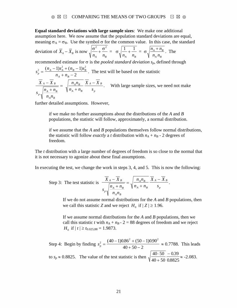
if we make no further assumptions about the distributions of the A and B populations, the statistic will follow, approximately, a normal distribution. if we assume that the A and B populations themselves follow normal distributions, the statistic will follow exactly a t distribution with nA + nB - 2 degrees of freedom.

The t distribution with a large number of degrees of freedom is so close to the normal that it is not necessary to agonize about these final assumptions. In executing the test, we change the work in steps 3, 4, and 5. This is now the following:

Step 3: The test statistic is X X

sn n

n n

n nn n

X Xs

A B

pA B

A B

A B

A B

A B

p

−+

=+

−.

If we do not assume normal distributions for the A and B populations, then we call this statistic Z and we reject H0 if | Z | ≥ 1.96. If we assume normal distributions for the A and B populations, then we call this statistic t with nA + nB - 2 = 88 degrees of freedom and we reject H0 if | t | ≥ t0.025;88 = 1.9873.

Step 4: Begin by finding sp2

2 240 1 0 86 50 1 0 9040 50 2

=− + −

+ −( ) . ( ) .

≈ 0.7788. This leads

to sp ≈ 0.8825. The value of the test statistic is then 40 5040 50

0 390 8825

⋅+

− ..

≈ -2.083.

Equal standard deviations with large sample sizes: We make one additional assumption here. We now assume that the population standard deviations are equal, meaning σA = σB. Use the symbol σ for the common value. In this case, the standard

deviation of X XA B− is now σ σ2 2

n nA B

+ = σ 1 1n nA B

+ = σ n nn nA B

A B

+ . The

recommended estimate for σ is the pooled standard deviation sp, defined through

sn s n s

n npA A B B

A B

22 21 1

2=

− + −+ −

( ) ( ). The test will be based on the statistic

p

BA

BA

BA

BA

BAp

BA

sXX

nnnn

nnnns

XX −+

=+

− . With large sample sizes, we need not make

further detailed assumptions. However,

COMPARING THE MEANS OF TWO GROUPS

22

Step 5: Whether we made the assumptions leading to Z or to t, the null hypotheses H0 would be rejected.

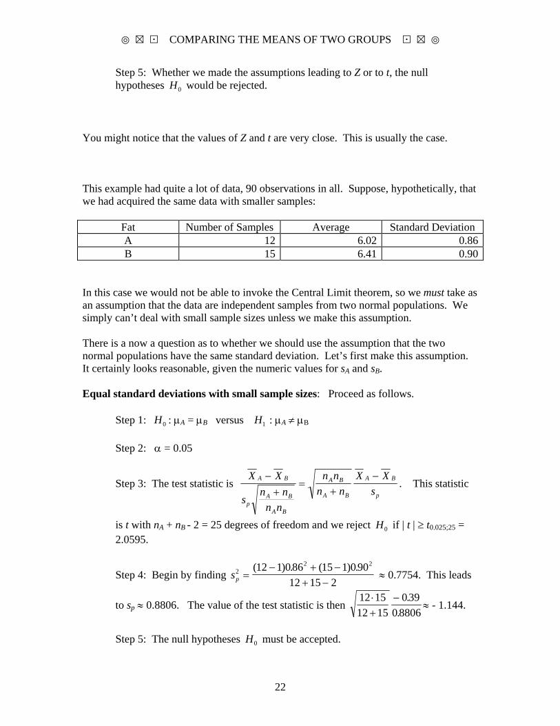
You might notice that the values of Z and t are very close. This is usually the case. This example had quite a lot of data, 90 observations in all. Suppose, hypothetically, that we had acquired the same data with smaller samples:

Fat Number of Samples Average Standard Deviation A 12 6.02 0.86B 15 6.41 0.90

In this case we would not be able to invoke the Central Limit theorem, so we must take as an assumption that the data are independent samples from two normal populations. We simply can’t deal with small sample sizes unless we make this assumption. There is a now a question as to whether we should use the assumption that the two normal populations have the same standard deviation. Let’s first make this assumption. It certainly looks reasonable, given the numeric values for sA and sB. Equal standard deviations with small sample sizes: Proceed as follows.

Step 1: H0 : μA = μB versus H1 : μA ≠ μB Step 2: α = 0.05

Step 3: The test statistic is X X

sn n

n n

n nn n

X Xs

A B

pA B

A B

A B

A B

A B

p

−+

=+

−. This statistic

is t with nA + nB - 2 = 25 degrees of freedom and we reject H0 if | t | ≥ t0.025;25 = 2.0595.

Step 4: Begin by finding sp2

2 212 1 0 86 15 1 0 9012 15 2

=− + −

+ −( ) . ( ) .

≈ 0.7754. This leads

to sp ≈ 0.8806. The value of the test statistic is then 12 1512 15

0 390 8806

⋅+

− ..

≈ - 1.144.

Step 5: The null hypotheses H0 must be accepted.

COMPARING THE MEANS OF TWO GROUPS

23

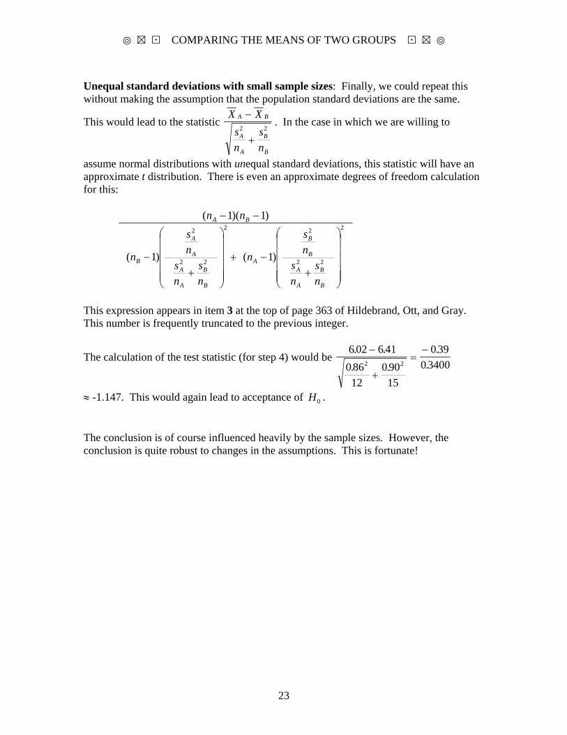
Unequal standard deviations with small sample sizes: Finally, we could repeat this without making the assumption that the population standard deviations are the same.

This would lead to the statistic X X

sn

sn

A B

A

A

B

B

−

+2 2

. In the case in which we are willing to

assume normal distributions with unequal standard deviations, this statistic will have an approximate t distribution. There is even an approximate degrees of freedom calculation for this:

2

22

22

22

2

)1()1(

)1)(1(

⎟⎟⎟⎟⎟

⎠

⎞

⎜⎜⎜⎜⎜

⎝

⎛

+−+

⎟⎟⎟⎟⎟

⎠

⎞

⎜⎜⎜⎜⎜

⎝

⎛

+−

−−

B

B

A

A

B

B

A

B

B

A

A

A

A

B

BA

ns

ns

ns

n

ns

ns

ns

n

nn

This expression appears in item 3 at the top of page 363 of Hildebrand, Ott, and Gray. This number is frequently truncated to the previous integer.

The calculation of the test statistic (for step 4) would be 6 02 6 41

0 8612

0 9015

0 390 34002 2

. .. .

..

−

+

=−

≈ -1.147. This would again lead to acceptance of H0 . The conclusion is of course influenced heavily by the sample sizes. However, the conclusion is quite robust to changes in the assumptions. This is fortunate!

COMPARING TWO GROUPS WITH MINITAB 14

24

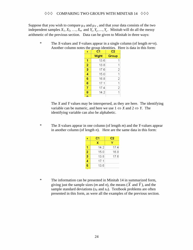
Suppose that you wish to compare μX and μY , and that your data consists of the two independent samples X1, X2, …, Xm and Y Y Yn1 2, , ..., . Minitab will do all the messy arithmetic of the previous section. Data can be given to Minitab in three ways:

* The X-values and Y-values appear in a single column (of length m+n). Another column notes the group identities. Here is data in this form:

The X and Y values may be interspersed, as they are here. The identifying variable can be numeric, and here we use 1 ⇔ X and 2 ⇔ Y. The identifying variable can also be alphabetic.

* The X-values appear in one column (of length m) and the Y-values appear in another column (of length n). Here are the same data in this form:

* The information can be presented in Minitab 14 in summarized form,

giving just the sample sizes (m and n), the means ( X and Y ), and the sample standard deviations (sX and sY). Textbook problems are often presented in this form, as were all the examples of the previous section.

COMPARING TWO GROUPS WITH MINITAB 14

25

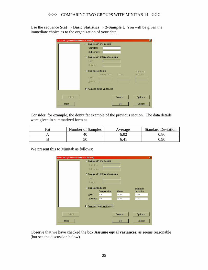
Use the sequence Stat ⇒ Basic Statistics ⇒ 2-Sample t. You will be given the immediate choice as to the organization of your data:

Consider, for example, the donut fat example of the previous section. The data details were given in summarized form as

Fat Number of Samples Average Standard Deviation A 40 6.02 0.86 B 50 6.41 0.90

We present this to Minitab as follows:

Observe that we have checked the box Assume equal variances, as seems reasonable (but see the discussion below).

COMPARING TWO GROUPS WITH MINITAB 14

26

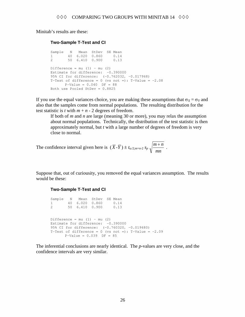
Minitab’s results are these:

Two-Sample T-Test and CI Sample N Mean StDev SE Mean 1 40 6.020 0.860 0.14 2 50 6.410 0.900 0.13 Difference = mu (1) - mu (2) Estimate for difference: -0.390000 95% CI for difference: (-0.762032, -0.017968) T-Test of difference = 0 (vs not =): T-Value = -2.08

P-Value = 0.040 DF = 88 Both use Pooled StDev = 0.8825

If you use the equal variances choice, you are making these assumptions that σX = σY and also that the samples come from normal populations. The resulting distribution for the test statistic is t with m + n - 2 degrees of freedom.

If both of m and n are large (meaning 30 or more), you may relax the assumption about normal populations. Technically, the distribution of the test statistic is then approximately normal, but t with a large number of degrees of freedom is very close to normal.

The confidence interval given here is ( X -Y ) ± tα/2;m+n-2 sp m nmn+ .

Suppose that, out of curiousity, you removed the equal variances assumption. The results would be these:

Two-Sample T-Test and CI Sample N Mean StDev SE Mean 1 40 6.020 0.860 0.14 2 50 6.410 0.900 0.13 Difference = mu (1) - mu (2) Estimate for difference: -0.390000 95% CI for difference: (-0.760320, -0.019680) T-Test of difference = 0 (vs not =): T-Value = -2.09

P-Value = 0.039 DF = 85

The inferential conclusions are nearly identical. The p-values are very close, and the confidence intervals are very similar.

COMPARING TWO GROUPS WITH MINITAB 14

27

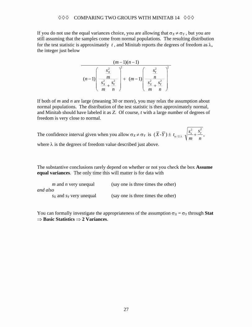
If you do not use the equal variances choice, you are allowing that σX ≠ σY , but you are still assuming that the samples come from normal populations. The resulting distribution for the test statistic is approximately t , and Minitab reports the degrees of freedom as λ, the integer just below

2 22 2

2 2 2 2

( 1)( 1)

( 1) ( 1)X Y

X Y X Y

m ns sm nn m

s s s sm n m n

− −

⎛ ⎞ ⎛ ⎞⎜ ⎟ ⎜ ⎟

− + −⎜ ⎟ ⎜ ⎟⎜ ⎟ ⎜ ⎟+ +⎜ ⎟ ⎜ ⎟⎝ ⎠ ⎝ ⎠

If both of m and n are large (meaning 30 or more), you may relax the assumption about normal populations. The distribution of the test statistic is then approximately normal, and Minitab should have labeled it as Z. Of course, t with a large number of degrees of freedom is very close to normal.

The confidence interval given when you allow σX ≠ σY is ( X -Y ) ± / 2;tα λ sm

sn

x y2 2

+ ,

where λ is the degrees of freedom value described just above. The substantive conclusions rarely depend on whether or not you check the box Assume equal variances. The only time this will matter is for data with

m and n very unequal (say one is three times the other) and also

sX and sY very unequal (say one is three times the other)

You can formally investigate the appropriateness of the assumption σX = σY through Stat ⇒ Basic Statistics ⇒ 2 Variances.

Does it matter which form of the two-sample t test we use?

28

The two-group comparison discussed in the section “Comparing the means of two groups” gets confusing because there are two different forms for the test.

If we are willing to assume σA = σB , we use A B

p

mn X Xm n s

−+

. The null distribution of

this statistic is tm+n-2 [*] .

If we wish to allow σA ≠ σB , we use 2 2

A B

A B

X Xs sm n

−

+

. Depending on nuanced assumptions,

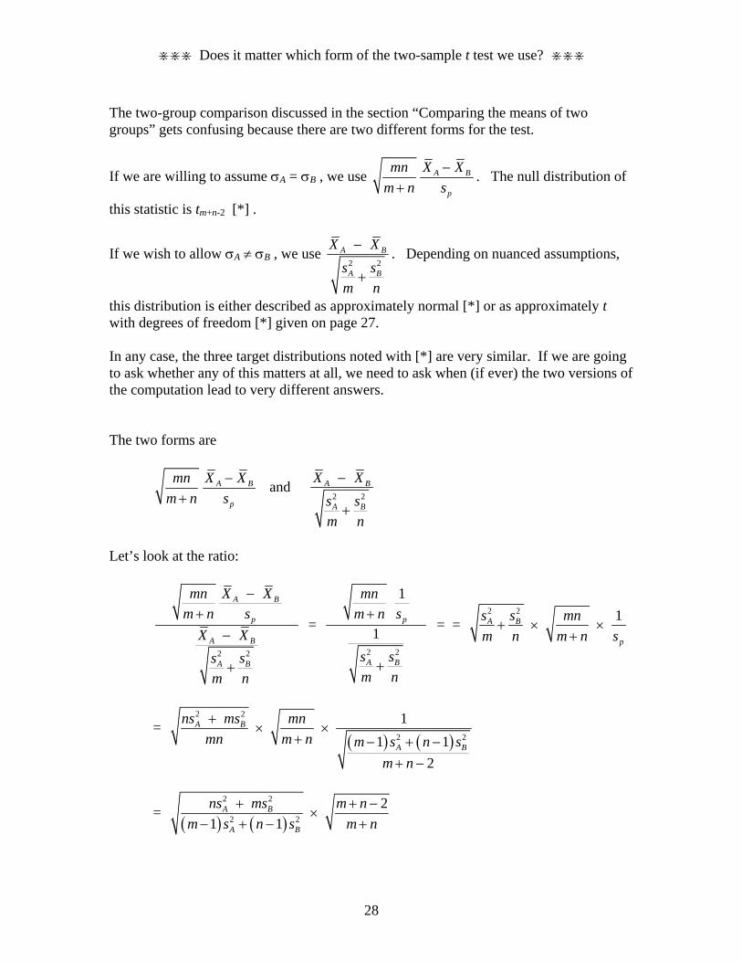
this distribution is either described as approximately normal [*] or as approximately t with degrees of freedom [*] given on page 27. In any case, the three target distributions noted with [*] are very similar. If we are going to ask whether any of this matters at all, we need to ask when (if ever) the two versions of the computation lead to very different answers. The two forms are

A B

p

mn X Xm n s

−+

and 2 2

A B

A B

X Xs sm n

−

+

Let’s look at the ratio:

2 2

A B

p

A B

A B

mn X Xm n s

X Xs sm n

−+

−

+

=

2 2

1

1p

A B

mnm n s

s sm n

+

+

= = 2 2 1A B

p

s s mnm n m n s+ × ×

+

= ( ) ( )

2 2

2 2

11 1

2

A B

A B

ns ms mnmn m n m s n s

m n

+× ×

+ − + −+ −

= ( ) ( )

2 2

2 2

21 1

A B

A B

ns ms m nm s n s m n

+ + −×

− + − +

Does it matter which form of the two-sample t test we use?

29

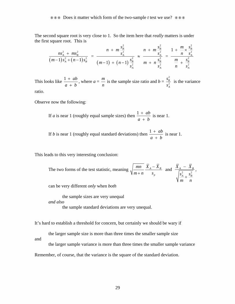
The second square root is very close to 1. So the item here that really matters is under the first square root. This is

( ) ( )2 2

2 21 1A B

A B

ns msm s n s

+− + −

= ( ) ( )

2

2

2

21 1

B

A

B

A

sn ms

sm ns

+

− + − ≈

2

2

2

2

B

A

B

A

sn mssm ns

+

+ =

2

2

2

2

1 B

A

B

A

m sn s

m sn s

+ ×

+

This looks like 1 aba b++

, where a = mn

is the sample size ratio and b = 2

2B

A

ss

is the variance

ratio. Observe now the following:

If a is near 1 (roughly equal sample sizes) then 1 aba b++

is near 1.

If b is near 1 (roughly equal standard deviations) then 1 aba b++

is near 1.

This leads to this very interesting conclusion:

The two forms of the test statistic, meaning A B

p

mn X Xm n s

−+

and 2 2

A B

A B

X Xs sm n

−

+

,

can be very different only when both

the sample sizes are very unequal and also

the sample standard deviations are very unequal.

It’s hard to establish a threshold for concern, but certainly we should be wary if

the larger sample size is more than three times the smaller sample size and

the larger sample variance is more than three times the smaller sample variance Remember, of course, that the variance is the square of the standard deviation.

Summary of hypothesis tests

30

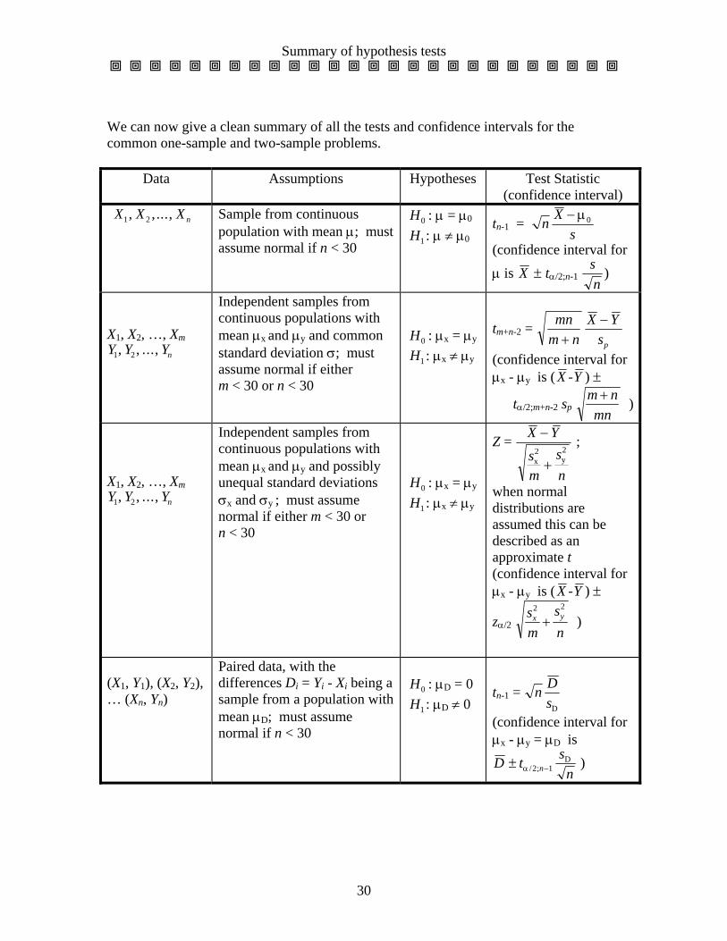
We can now give a clean summary of all the tests and confidence intervals for the common one-sample and two-sample problems.

Data Assumptions Hypotheses Test Statistic (confidence interval)

X X X n1 2, , ..., Sample from continuous population with mean μ; must assume normal if n < 30

H0 : μ = μ0

H1 : μ ≠ μ0 tn-1 = n X

s− μ0

(confidence interval for

μ is X ± tα/2;n-1 sn

)

X1, X2, …, Xm Y Y Yn1 2, , ...,

Independent samples from continuous populations with mean μx and μy and common standard deviation σ; must assume normal if either m < 30 or n < 30

H0 : μx = μy

H1 : μx ≠ μy

tm+n-2 = mnm n

X Ysp+−

(confidence interval for μx - μy is ( X -Y ) ±

tα/2;m+n-2 sp m nmn+ )

X1, X2, …, Xm Y Y Yn1 2, , ...,

Independent samples from continuous populations with mean μx and μy and possibly unequal standard deviations σx and σy ; must assume normal if either m < 30 or n < 30

H0 : μx = μy

H1 : μx ≠ μy

Z = X Ysm

sn

−

+x2

y2

;

when normal distributions are assumed this can be described as an approximate t (confidence interval for μx - μy is ( X -Y ) ±

zα/2 sm

sn

x y2 2

+ )

(X1, Y1), (X2, Y2), … (Xn, Yn)

Paired data, with the differences Di = Yi - Xi being a sample from a population with mean μD; must assume normal if n < 30

H0 : μD = 0 H1 : μD ≠ 0

tn-1 = n DsD

(confidence interval for μx - μy = μD is

D t snn± −α / ;2 1D )

Summary of hypothesis tests

31

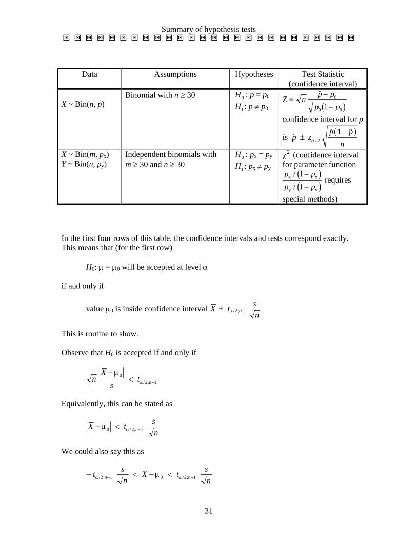
Data Assumptions Hypotheses Test Statistic (confidence interval)

X ~ Bin(n, p)

Binomial with n ≥ 30 H0 : p = p0 H1 : p ≠ p0

Z = n p pp p−

−0

0 01b g confidence interval for p

is p ± ( )/ 2

1p pz

nα

−

X ~ Bin(m, px) Y ~ Bin(n, py)

Independent binomials with m ≥ 30 and n ≥ 30

H0 : px = py H1 : px ≠ py

χ2 (confidence interval

for parameter function p pp p

x x

y y

//

11−

−b gc h requires

special methods) In the first four rows of this table, the confidence intervals and tests correspond exactly. This means that (for the first row)

H0: μ = μ0 will be accepted at level α if and only if

value μ0 is inside confidence interval X ± tα/2;n-1 sn

This is routine to show. Observe that H0 is accepted if and only if

nX

st n

−< −

μα

02 1/ ;

Equivalently, this can be stated as

X t snn− < −μ α0 2 1/ ;

We could also say this as

− < − <− −t sn

X t snn nα αμ/ ; / ;2 1 0 2 1

Summary of hypothesis tests

32

This last inequality can be rearranged as

X t sn

X t snn n− < < +− −α αμ/ ; / ;2 1 0 2 1

This is precisely the condition that μ0 is inside the confidence interval. Now let’s deal with the binomial random variable X with n and π. In general we don’t

know π, so we use the estimate π = Xn

. We also noted that SE(π ) = π π1−b g

n. We had

the 1-α confidence interval by the Agrest-Coull method. Now let’s consider a test of the null hypothesis H0: π = π0, where π0 is some specified comparison value. The alternative will be H1: π ≠ π0. If you like one-sided tests, then you can modify all this stuff in the obvious way. If H0 is true, then the SD of π is π π0 01−b g

n. This is not a standard error. If H0 holds, then we don’t have to estimate

SD(π ). Thus it follows, if the sample size is reasonably large, that the distribution of

Z = π ππ

− 0

SDb g is approximately standard normal. This leads to the test based on Z.

What are the Uses for Hypothesis Tests?

33

To what uses can we put hypothesis tests? This is an interesting question, because we often have alternate ways of dealing with data. We could use our data to test the null hypothesis H0: θ = θ0 against an alternative H1.

Here θ is the true-but-unknown parameter, and θ0 is a specified comparison value. In most cases θ0 is an obvious baseline value (zero for a regression coefficient, one for a risk ratio, zero for a product difference, and so on). The alternative could be H1: θ ≠ θ0 , which is called a two-sided (or two-tailed) alternative. In many cases H1: θ > θ0 because we are interested only in θ-values which are larger than θ0 . This is called a one-sided (or one-tailed) alternative. There are also cases H1: θ < θ0 because we are interested only in θ-values which are smaller than θ0 ; these cases are also called one-sided.

In most cases, the two-sided version of H1 is preferred, unless there is obvious a priori interest in a one-sided statement. This formalization has to be part of the investigation protocol. It is considered unacceptable to specify H1 after an examination of the data.

The most obvious competitor for a hypothesis test is a confidence interval. This is a statement of the form “I am 95% confident that the true-but-unknown value of θ is in the interval 38.5 ± 8.4.” In any application, this interval is given numerically, but you will

encounter algebraic forms such as x ± / 2; 1nstnα − .

The hypothesis test seems to make a yes-or-no decision about H0 , while the confidence interval makes a data-based suggestion as to the location of θ. It is important to note that either of these methods could be in error.

The confidence interval might not include the true value of θ. If you routinely use 95% confidence intervals, then in the long run about 5% of your intervals will not contain the target value. This is understood, and it’s implicit in the notion of 95% confidence.

The hypothesis test might lead to a wrong decision.

(1) If H0 is correct and you end up rejecting H0, then you have made a Type I error. From a statistical point of view, we try to control this error, and tests use the notion of level of significance as an upper bound on the probability of Type I error. This upper bound is usually called α, and its value is most often 0.05. We design the test so that

P[ reject H0 | H0 true ] ≤ α

What are the Uses for Hypothesis Tests?

34

Statisticians are very much aware of this type of error, and some are reluctant to utter the phrase “I reject the null hypothesis.” These people will use phrases like “the results are statistically significant.”

In the legal comparison, a Type I error corresponds to finding the defendant guilty when in fact the defendant is innocent. The law certainly finds α = 0.05 too high for use in a criminal trial, but the 0.05 standard can be used in relation to monetary awards

(2) If H0 is incorrect and you end up accepting H0 , then you have

made a Type II error. As the hypothesis testing game has been set up, it is very hard to give numbers for Type II error. This happens because there are many ways for H0 to be false.

Suppose that you are testing H0: θ = 400 versus H1: θ ≠ 400 and you have a sample of n = 40 data points. You are very unlikely to make a Type II error if the true value of θ is 900, but you have a large probability of Type II error if the true value of θ is 402. Most hypothesis tests operate so that the probability of Type II error drops as n grows. A sample of size n = 50 is better than a sample of size n = 40, whether θ is 900 or 402.

Statisticians are aware of this type of error as well, and some do not like to say “I accept the null hypothesis.” Alternate phrases are “the results are not statistically significant,” “I cannot reject the null hypothesis,” or “I reserve judgment.”

So how do hypothesis tests get used? Some situations call for a clear accept-or-reject action. We might have to decide which make of photocopier to use when the current contract expires. We might have to decide whether an environmentally sensitive lake should be opened for sport fishing for the next season. These situations require a careful evaluation of the costs and an appreciation for the consequences of Type I and Type II errors. Legal decisions are of course in this context. Some situations ask for an opinion about whether a relationship exists. For example, in a regression of Y on X, using the model Yi = β0 + β1 Xi + εi , it’s common to test the null hypothesis H0 : β1 = 0 against H1: β1 ≠ 0. We do this to see if there is a relationship between X and Y. It’s possible that no actions will be associated with the decisions, and we’re doing all this just to satisfy our curiosity.

What are the Uses for Hypothesis Tests?

35

If X is a policy variable and if Y is a consequence, the result of the hypothesis test might decide our future actions. Even so, it might be much more useful to have a confidence interval for β1, a quantitative assessment of the relationship.

As noted above, the probability of making a Type II error depends on the true value of θ and depends also on the sample size n. The following symbols and expressions are used in describing items related to Type II error:

β = P[ Type II error ] Beta depends on the true value of θ and depends also on n.

1 - β This is the power of the test. It depends on the true

value of θ and also on n. β(θ) = power curve This assumes that the sample size n has been fixed,

and it gives the probability of rejecting H0 as a function of θ.

The function 1 - β(θ) is called the operating characteristic curve, or the OC curve. (This terminology is not universal.)

Pictures of the power curve are very interesting. Suppose that we have a single sample x1, x2, … , xn and we wish to test the null hypothesis H0: θ = population mean = 400 versus alternative H1: θ ≠ 400. The conventional statistical procedure is the t test, based on the statistic

t = 400xns−

Here x represents the sample mean and s represents the sample standard deviation. This kind of test is usually done at the 0.05 significance level. This means, to an excellent approximation, that

we will be led to accept H0 if -2 ≤ t ≤ 2 we will be led to reject H0 if | t | > 2

Suppose that the data produce x = 410 and s = 98 with a sample of n = 50. The value of

the t statistic would be 410 4005098− ≈ 0.72. This value would lead to accepting H0 ;

the data are not able to convince us that the population mean θ is not 400. The departure of the data value x from the target value 400 is simply not shocking.

What are the Uses for Hypothesis Tests?

36

Suppose though that we produced the same x = 410 and the same s = 98, but we did this

with a sample of n = 500. This time the t statistic would be 410 40050098− ≈ 2.28 and

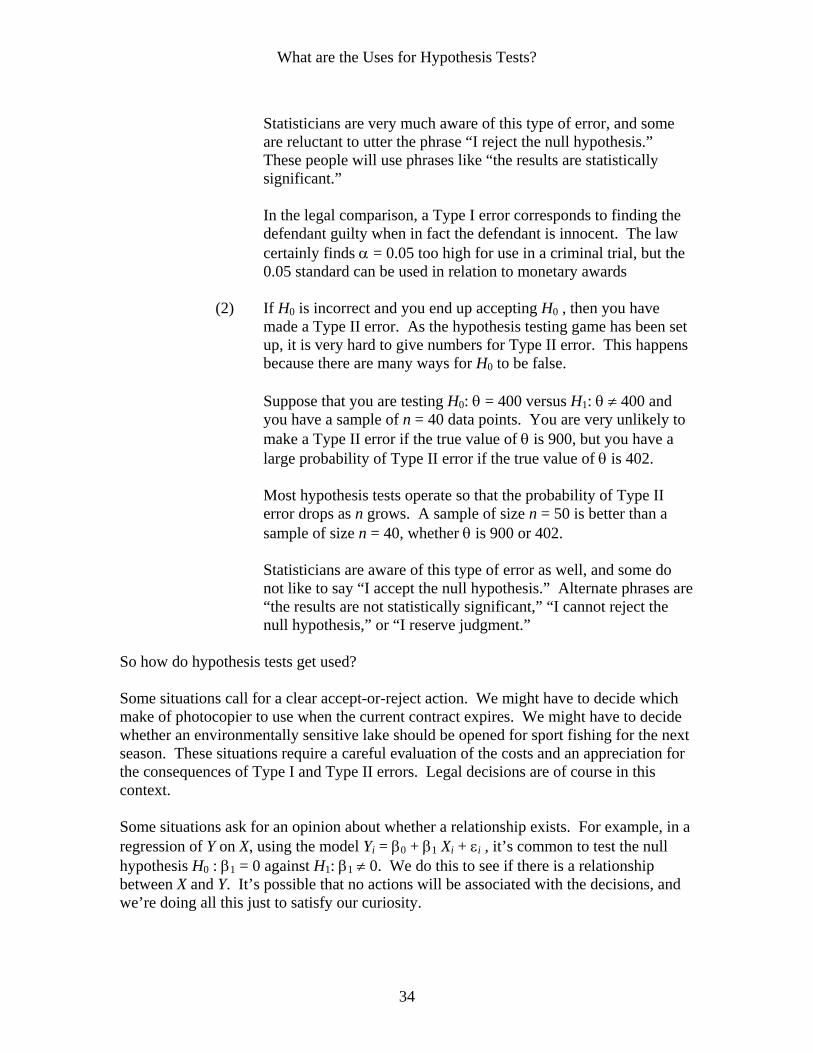
we would be led to rejecting H0 . Perhaps the population mean θ really is near 410. This is a short distance from 400, in light of the size of the standard deviation. The larger sample size gives us the ability to make a smaller difference significant. It can be proved that, if H0 is correct, then the probability of incorrectly rejecting H0 (thus committing Type I error) will be exactly 0.05 no matter what the sample size. The behavior of this procedure when H0 is false can be seen best by examining the power curve. Suppose that the population standard deviation is σ = 100. This neatly matches the sample standard deviation s = 98 in the example. The graph below gives the power, meaning the probability of rejecting H0. The sample size has been fixed here at n = 50.

500-50

1.0

0.9

0.80.7

0.6

0.50.4

0.3

0.20.1

0.0

Pow

er

Difference, theta minus theta-0

One-sample t test, alpha = 0.05, sigma = 100, n = 50

If the difference between the true θ and the comparison value 400 is about 10, and if the true standard deviation of the population is 100, there is only about a 15% probability of rejecting H0 . Here’s another way to say this: if H0 is false with the actual θ being 410, then this procedure has only a 15% chance of doing the right thing. This test has low power when the alternative value is 410.

What are the Uses for Hypothesis Tests?

37

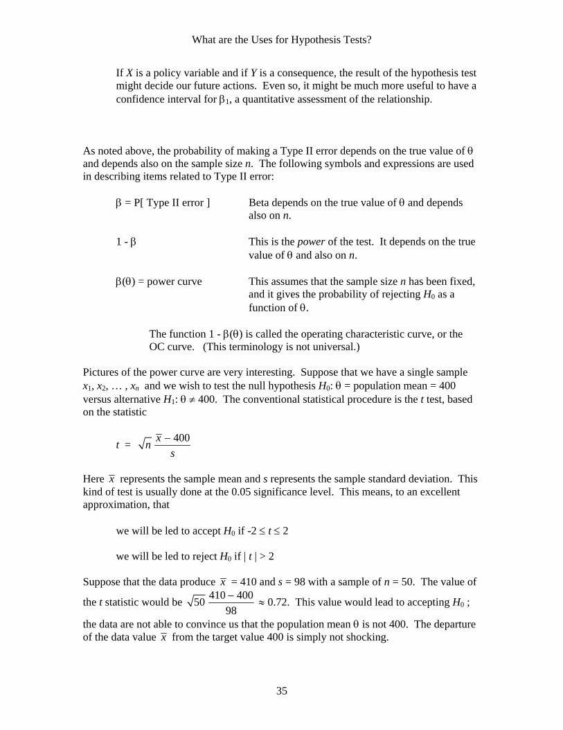
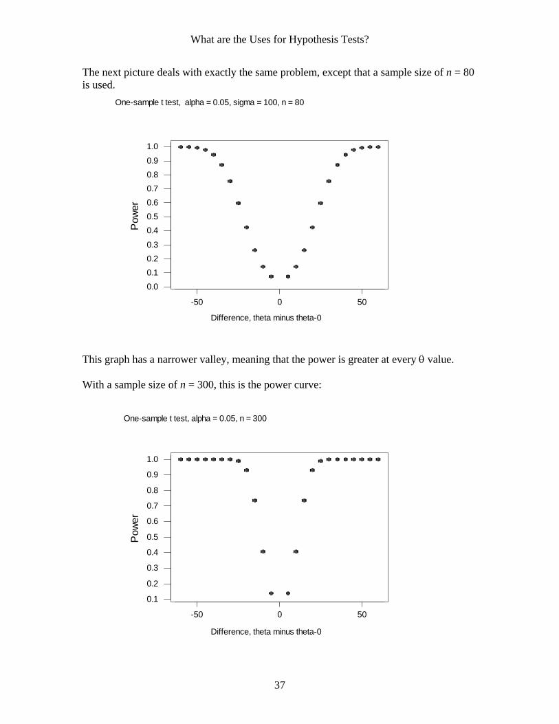
The next picture deals with exactly the same problem, except that a sample size of n = 80 is used.

500-50

1.0

0.90.80.70.60.50.4

0.30.20.10.0

Pow

er

Difference, theta minus theta-0

One-sample t test, alpha = 0.05, sigma = 100, n = 80

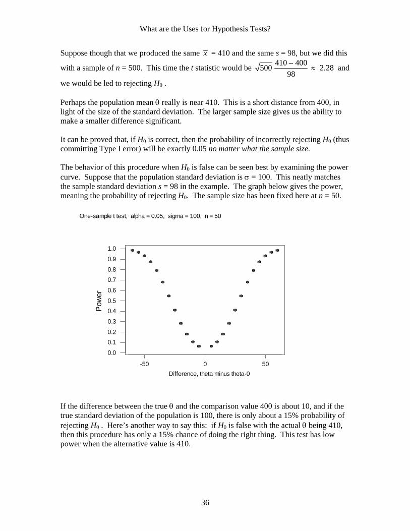
This graph has a narrower valley, meaning that the power is greater at every θ value. With a sample size of n = 300, this is the power curve:

500-50

1.0

0.9

0.8

0.7

0.6

0.5

0.4

0.3

0.2

0.1

Pow

er

Difference, theta minus theta-0

One-sample t test, alpha = 0.05, n = 300

What are the Uses for Hypothesis Tests?

38

All curves have their bottoms at the point (0, 0.05), corresponding to the 0.05 probability of rejecting H0 when it is true. So here are some useful points:

* The power is greater if θ is far from the comparison value specified by the null hypothesis.

* The power is greater if the sample size n is larger. * If you want to accept H0 you should try to use a small sample size. * If you want to reject H0 you should try to use a large sample size.

Suppose that the problem is to test the null hypothesis H0: θ = 400 versus alternative H1: θ ≠ 400. Suppose that, in advance of collecting the data, you believe that the true value of θ is near 410 and that the population standard deviation is near 100.

If you would really like to see that H0 is accepted, then you would look at the first picture above and note that n = 50 is very likely to lead to accepting H0 . You will recommend a sample of size 50. If you would like to see that H0 is rejected, then you would look at a series (varying over n) of pictures like those here until you get one with high power when θ is near 410 and the standard deviation is near 100. You will recommend a sample of size 500. Technically, there’s a formula that can be used for this purpose, so you do not have to create and examine all these graphs.

There is an obvious tension here. This tension will be resolved in a legal sense by the requirement that the statistical procedure have enough power to detect reasonably interesting alternative hypotheses. This still leaves plenty of room to haggle. After all, we have to decide what “reasonably interesting” means. In the example given here, θ = 410 (relative to σ = 100) would probably not be deemed reasonably interesting, as it

is only 410 400100− = 0.1 of a standard deviation off the null hypothesis. Certainly

θ = 450 would be considered reasonably interesting.