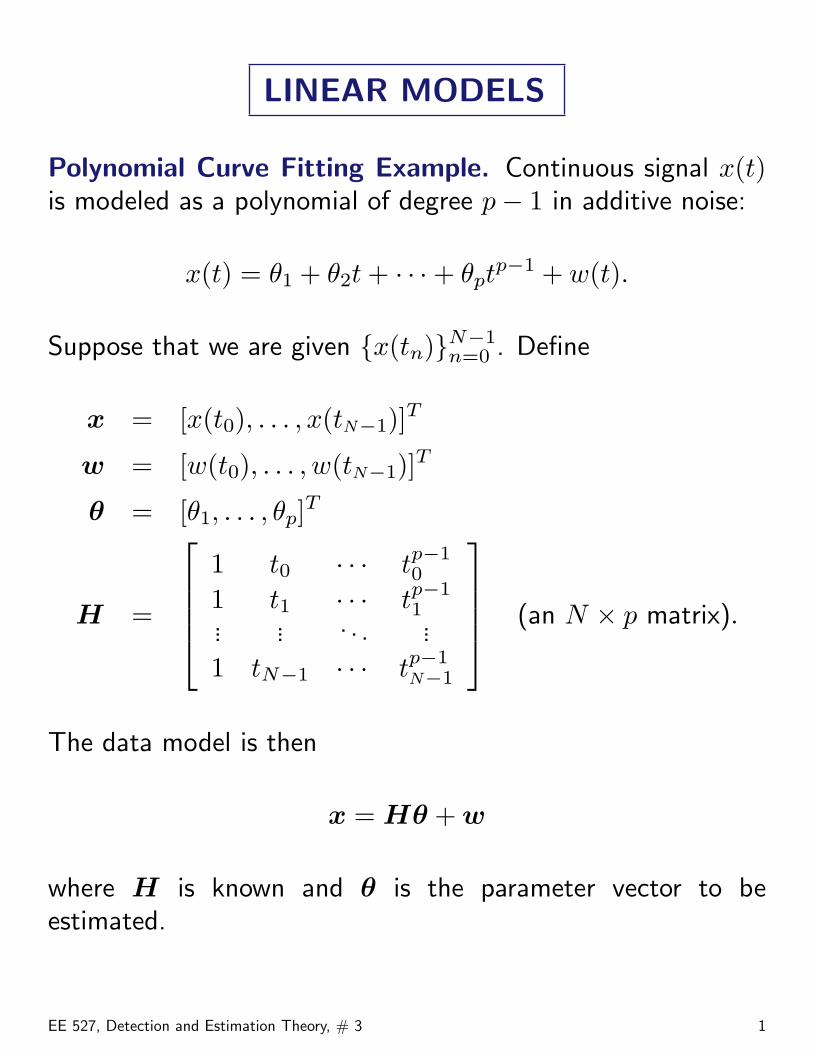
LINEAR MODELS

Polynomial Curve Fitting Example. Continuous signal x(t)is modeled as a polynomial of degree p− 1 in additive noise:

x(t) = θ1 + θ2t + · · ·+ θptp−1 + w(t).

Suppose that we are given {x(tn)}N−1n=0 . Define

x = [x(t0), . . . , x(tN−1)]T

w = [w(t0), . . . , w(tN−1)]T

θ = [θ1, . . . , θp]T

H =

1 t0 · · · tp−1

0

1 t1 · · · tp−11

... ... . . . ...

1 tN−1 · · · tp−1N−1

(an N × p matrix).

The data model is then

x = Hθ + w

where H is known and θ is the parameter vector to beestimated.

EE 527, Detection and Estimation Theory, # 3 1

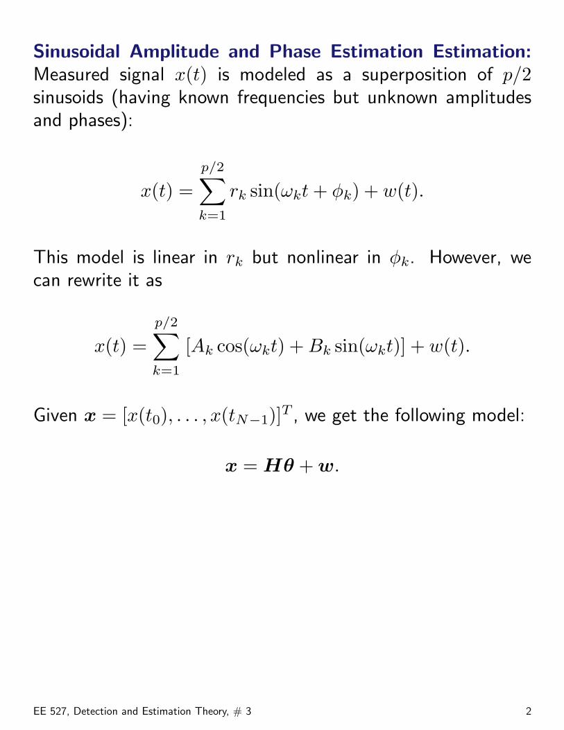
Sinusoidal Amplitude and Phase Estimation Estimation:Measured signal x(t) is modeled as a superposition of p/2sinusoids (having known frequencies but unknown amplitudesand phases):

x(t) =p/2∑k=1

rk sin(ωkt + φk) + w(t).

This model is linear in rk but nonlinear in φk. However, wecan rewrite it as

x(t) =p/2∑k=1

[Ak cos(ωkt) + Bk sin(ωkt)] + w(t).

Given x = [x(t0), . . . , x(tN−1)]T , we get the following model:

x = Hθ + w.

EE 527, Detection and Estimation Theory, # 3 2

Linear Models (cont.)

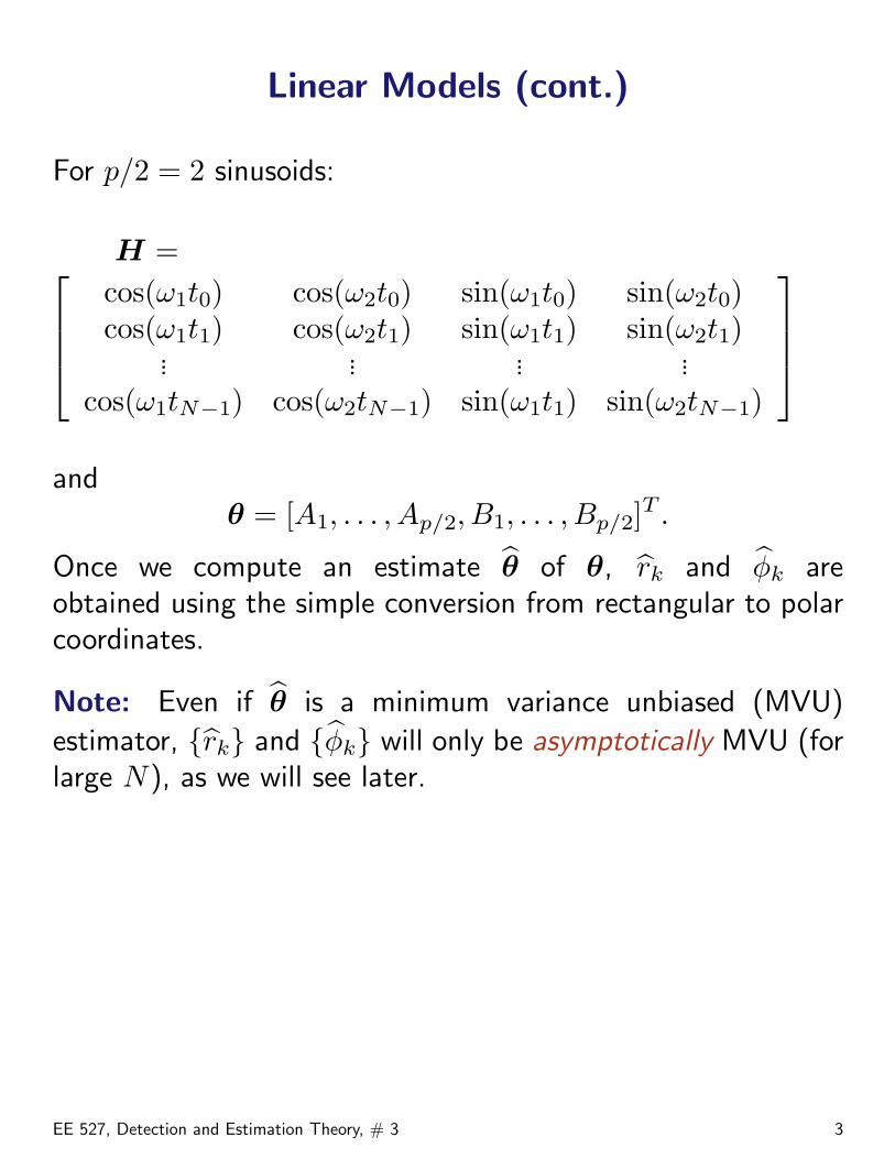
For p/2 = 2 sinusoids:

H =cos(ω1t0) cos(ω2t0) sin(ω1t0) sin(ω2t0)cos(ω1t1) cos(ω2t1) sin(ω1t1) sin(ω2t1)

... ... ... ...cos(ω1tN−1) cos(ω2tN−1) sin(ω1t1) sin(ω2tN−1)

and

θ = [A1, . . . , Ap/2, B1, . . . , Bp/2]T .

Once we compute an estimate θ of θ, rk and φk areobtained using the simple conversion from rectangular to polarcoordinates.

Note: Even if θ is a minimum variance unbiased (MVU)

estimator, {rk} and {φk} will only be asymptotically MVU (forlarge N), as we will see later.

EE 527, Detection and Estimation Theory, # 3 3

General Problem Formulation

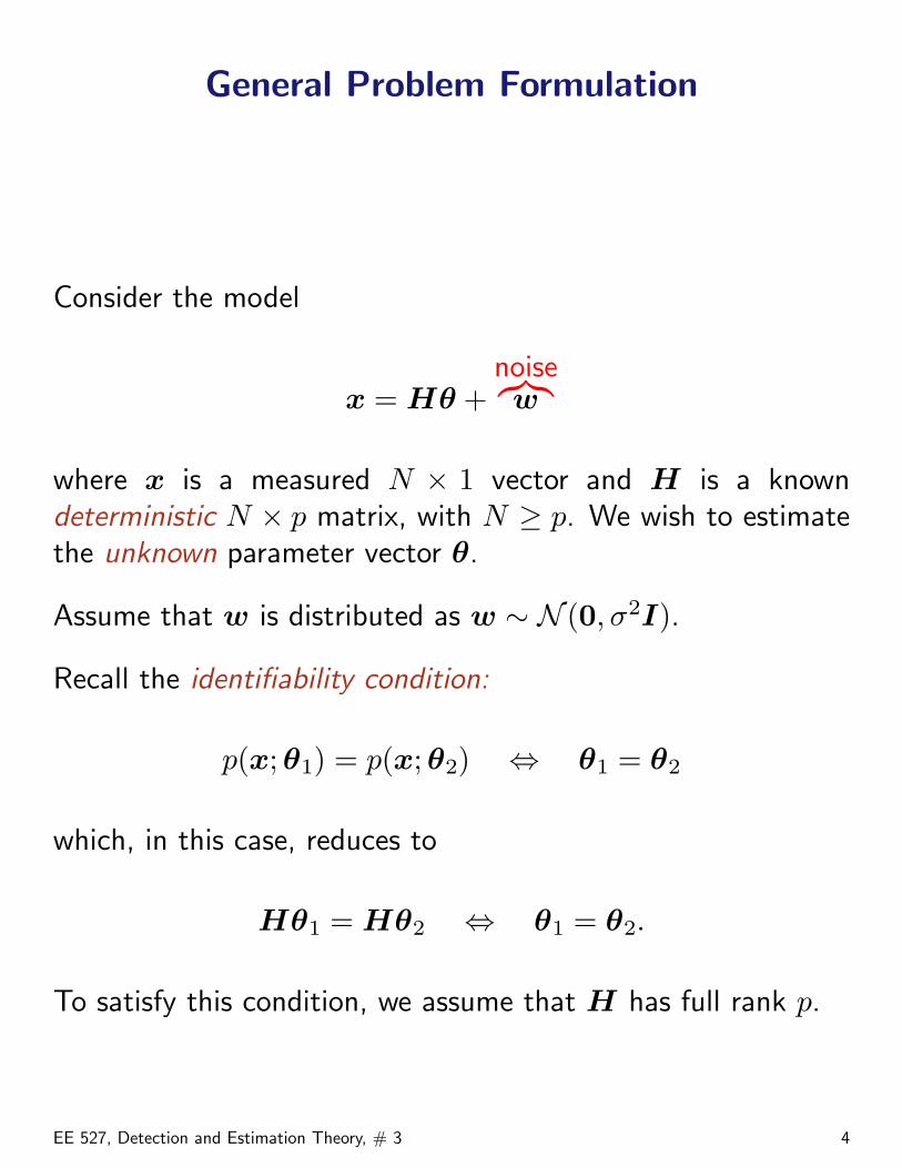
Consider the model

x = Hθ +noise︷︸︸︷w

where x is a measured N × 1 vector and H is a knowndeterministic N × p matrix, with N ≥ p. We wish to estimatethe unknown parameter vector θ.

Assume that w is distributed as w ∼ N (0, σ2I).

Recall the identifiability condition:

p(x;θ1) = p(x;θ2) ⇔ θ1 = θ2

which, in this case, reduces to

Hθ1 = Hθ2 ⇔ θ1 = θ2.

To satisfy this condition, we assume that H has full rank p.

EE 527, Detection and Estimation Theory, # 3 4

Minimum Variance Unbiased Estimator for theLinear Model

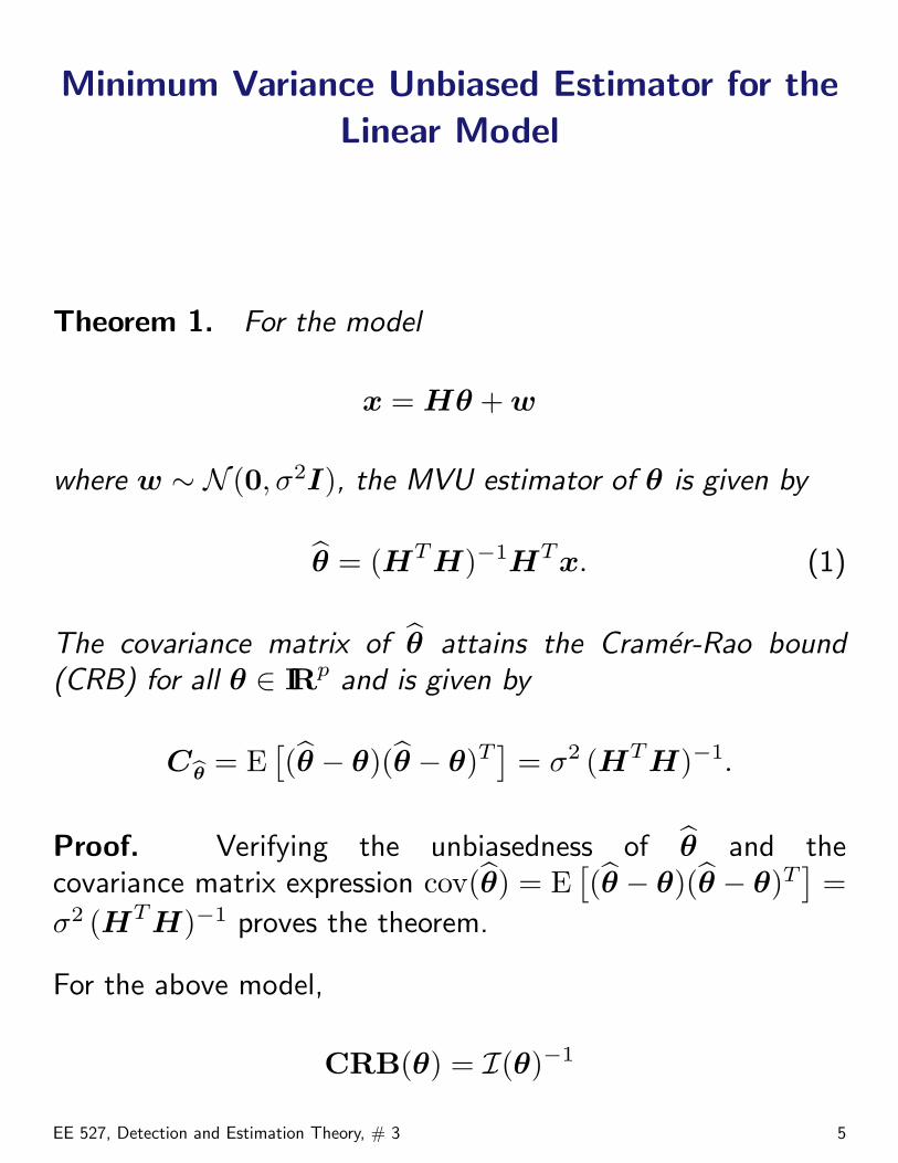
Theorem 1. For the model

x = Hθ + w

where w ∼ N (0, σ2I), the MVU estimator of θ is given by

θ = (HTH)−1HTx. (1)

The covariance matrix of θ attains the Cramer-Rao bound(CRB) for all θ ∈ RI p and is given by

Cbθ = E[(θ − θ)(θ − θ)T

]= σ2 (HTH)−1.

Proof. Verifying the unbiasedness of θ and thecovariance matrix expression cov(θ) = E

[(θ − θ)(θ − θ)T

]=

σ2 (HTH)−1 proves the theorem.

For the above model,

CRB(θ) = I(θ)−1

EE 527, Detection and Estimation Theory, # 3 5

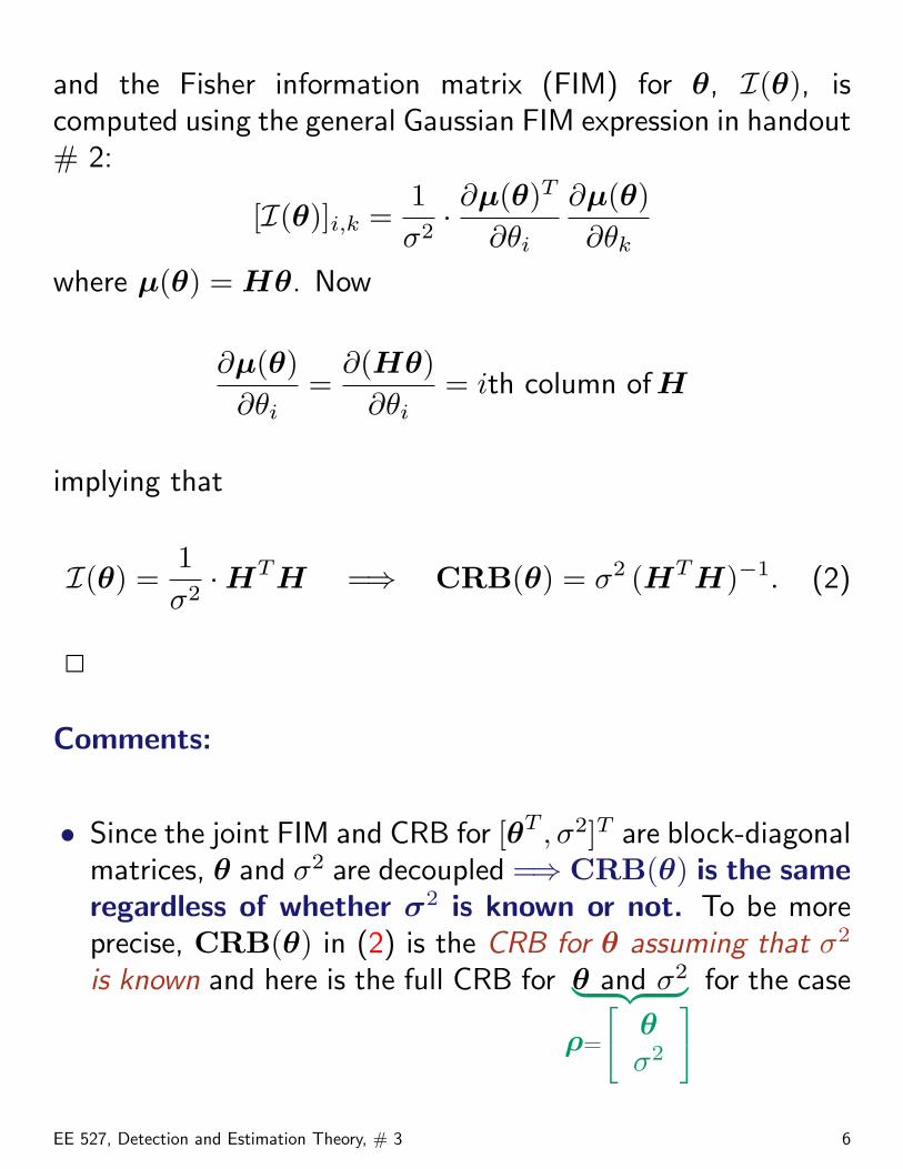
and the Fisher information matrix (FIM) for θ, I(θ), iscomputed using the general Gaussian FIM expression in handout# 2:

[I(θ)]i,k =1σ2· ∂µ(θ)T

∂θi

∂µ(θ)∂θk

where µ(θ) = Hθ. Now

∂µ(θ)∂θi

=∂(Hθ)

∂θi= ith column ofH

implying that

I(θ) =1σ2·HTH =⇒ CRB(θ) = σ2 (HTH)−1. (2)

2

Comments:

• Since the joint FIM and CRB for [θT , σ2]T are block-diagonalmatrices, θ and σ2 are decoupled =⇒ CRB(θ) is the sameregardless of whether σ2 is known or not. To be moreprecise, CRB(θ) in (2) is the CRB for θ assuming that σ2

is known and here is the full CRB for θ and σ2︸ ︷︷ ︸ρ=

24 θσ2

35for the case

EE 527, Detection and Estimation Theory, # 3 6

where both θ and σ2 are unknown:

CRBρ,ρ(θ, σ2) =

same as (2)︷ ︸︸ ︷CRBθθ(θ, σ2) 0

0 CRBσ2,σ2(σ2)

.

Therefore, θ in (1) is the MVU estimator of θ regardless ofwhether σ2 is known or not.

• θ in (1) coincides with the least-squares (LS) estimate of θ:

θ = arg minθ‖x−Hθ‖2

which can be shown by differentiating ‖x − Hθ‖2 withrespect to θ and setting the result to zero or by completingthe squares. Later in this handout, we will see a geometricinterpretation of the LS approach.

EE 527, Detection and Estimation Theory, # 3 7

Minimum Variance Unbiased Estimator for theLinear Model (cont.)

The solution from the above theorem is numerically not soundas given. It is better to use a QR factorization, say, brieflyoutlined below. Suppose that the N × p matrix H is factoredas

H = QR = [Q1 Q2][

R1

0

]= Q1R1

where Q is orthonormal and R1 is upper triangular p × p(Matlab: qr). Then

(HTH)−1HT = R−11 QT

1 .

Thus, θ can be obtained by solving the triangular system ofequations

R1θ = QT1 x.

Matlab has the “backslash” command for computing the LSsolution:

θ = H\x;

EE 527, Detection and Estimation Theory, # 3 8

Minimum Variance Unbiased Estimator for theLinear Model, Colored Noise

Suppose that we have colored noise, so that w ∼ N (0, σ2 C),where C 6= I is known and positive definite.

We can use prewhitening to get back to the old problem (i.e.the white-noise case). We compute the Cholesky factorizationof C−1:

C−1 = DTD Matlab: D = inv(chol(C))’;

(Any other square-root factorization could be used as well.)

Now, define the transformed measurement model:

D x︸︷︷︸xtransf

= D H︸ ︷︷ ︸H transf

θ + D w︸︷︷︸wtransf

.

Clearly, wtransf ∼ N (0, σ2I) and the problem is reduced tothe white-noise case.

EE 527, Detection and Estimation Theory, # 3 9

MVU Estimation, Colored Noise (cont.)

Theorem 2. For colored Gaussian noise with knowncovariance C, the MVU estimate of θ is

θ = (HTC−1H)−1HTC−1x.

The covariance matrix of θ attains the CRB and is given by

Cbθ = (HTC−1H)−1.

Note: θ is a weighted LS estimate,

θ = arg minθ‖x−Hθ‖2W

= arg minθ

(x−Hθ)T W (x−Hθ).

The “optimal weight matrix,” W = C−1, prewhitens theresiduals.

EE 527, Detection and Estimation Theory, # 3 10

Best Linear Unbiased Estimator

Given the modelx = Hθ + w (3)

where w has zero mean and covariance matrix E [wwT ] = C,we look for the best linear unbiased estimator (BLUE). Hence,we restrict our estimator to be

• linear (i.e. of the form θ = ATx) and

• unbiased

and minimize its variance.

Theorem 3. (Gauss-Markov) The BLUE of θ is

θ = (HTC−1H)−1HTC−1x

and its covariance matrix is

Cbθ = (HTC−1H)−1.

The expression for Cbθ holds independently of the distributionof w — all we impose on w is that it has known mean vectorand covariance matrix, equal to 0 and C (respectively).

EE 527, Detection and Estimation Theory, # 3 11

The estimate θ is (statistically) efficient if w is Gaussian (i.e.it attains the CRB), but it is not efficient in general. Fornon-Gaussian measurement models, there might be a betternonlinear estimate. (Most likely, there exists a better nonlinearestimate.)

Proof. (of Theorem 3). For simplicity, consider first the casewhere θ is scalar. Then, our measurement model is

x[n] = h[n] θ + w[n] ⇐⇒ x = h θ + w.

The candidate linear estimates of θ have the following form:

θ =N−1∑n=0

anx[n] = aTx.

First, the bias is computed:

E [θ] = aTE [x] = aTh θ.

Thus, θ is unbiased if and only if aTh = 1. Next, compute thevariance of θ. We have

θ − θ = aT (h θ + w︸ ︷︷ ︸x

)− θ = aTw

EE 527, Detection and Estimation Theory, # 3 12

where we have used the unbiasedness condition: aTh = 1.Therefore, the variance is

E [(θ − θ)2] = E [(aTw)2] = E [aTwwTa] = aTCa.

Note: The variance of θ depends only on the second-orderproperties of the noise. This result holds for any noisedistribution that has second-order moments.

Thus, the BLUE problem is

mina

aTCa such that aTh = 1.

Note the equivalence with MVDR beamforming. To read moreabout MVDR beamforming, see

H.L. Van Trees, Detection, Estimation and ModulationTheory, New York: Wiley, 2002, pt. IV.

Lagrange-multiplier formulation:

L(a) = aTCa+λ·(aTh−1) differentiate=⇒ 2 Ca+λ h = 0.

Hence

a = −λ

2·C−1h

and then

aTh = −λ

2hTC−1h = 1 ⇒ λ = − 2

hTC−1h

EE 527, Detection and Estimation Theory, # 3 13

and optimal a follows: a = (hTC−1h)−1C−1h. Returning toour estimator, we find the BLUE to be

θ = (hTC−1h)−1hTC−1x.

and its variance is given by

E [(θ − θ)2] = (hTC−1h)−1.

2

Consider the vector case. Linear unbiased estimates of θ:

θ = ATx, where A is independent of x. (4)

Remark: For LS estimate θLS, AT = (HTH)−1HT .

θ = E [θ] = E [ATx] = E [AT (Hθ + w)] = ATHθ.

⇒ ATH = I.

Remark: For BLUE θBLUE, ATBLUE = (HTC−1H)−1HTC−1.

Since ATBLUEH = I ⇒ E [θBLUE] = θ.

cov(θ) = E {[AT (Hθ + w︸ ︷︷ ︸x

)−θ][AT (Hθ+w)−θ]T} = ATCA.

EE 527, Detection and Estimation Theory, # 3 14

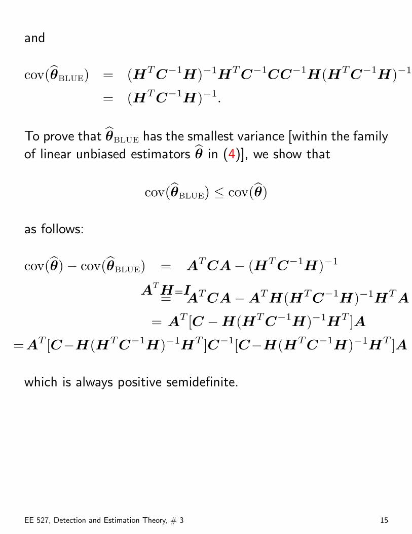
and

cov(θBLUE) = (HTC−1H)−1HTC−1CC−1H(HTC−1H)−1

= (HTC−1H)−1.

To prove that θBLUE has the smallest variance [within the family

of linear unbiased estimators θ in (4)], we show that

cov(θBLUE) ≤ cov(θ)

as follows:

cov(θ)− cov(θBLUE) = ATCA− (HTC−1H)−1

ATH=I= ATCA−ATH(HTC−1H)−1HTA

= AT [C −H(HTC−1H)−1HT ]A

=AT [C−H(HTC−1H)−1HT ]C−1[C−H(HTC−1H)−1HT ]A

which is always positive semidefinite.

EE 527, Detection and Estimation Theory, # 3 15

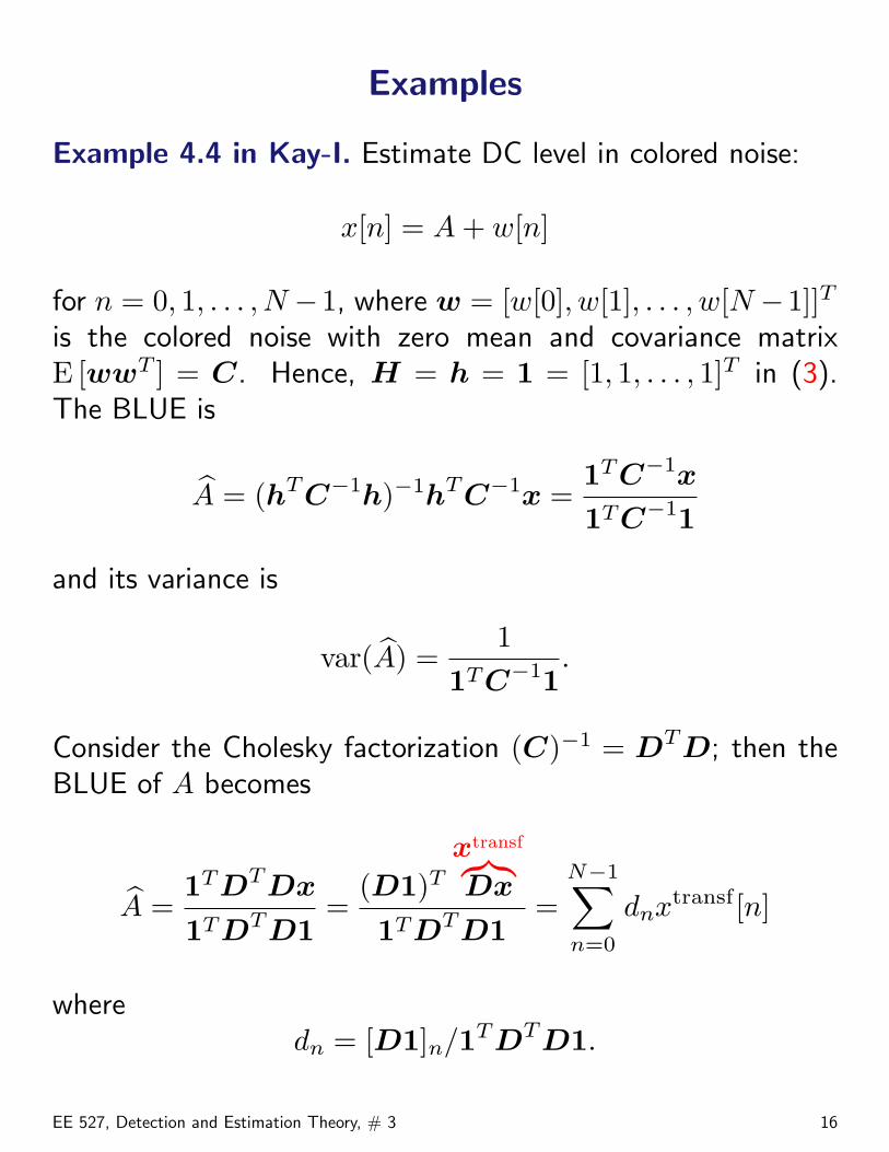
Examples

Example 4.4 in Kay-I. Estimate DC level in colored noise:

x[n] = A + w[n]

for n = 0, 1, . . . , N −1, where w = [w[0], w[1], . . . , w[N −1]]T

is the colored noise with zero mean and covariance matrixE [wwT ] = C. Hence, H = h = 1 = [1, 1, . . . , 1]T in (3).The BLUE is

A = (hTC−1h)−1hTC−1x =1TC−1x

1TC−11

and its variance is

var(A) =1

1TC−11.

Consider the Cholesky factorization (C)−1 = DTD; then theBLUE of A becomes

A =1TDTDx

1TDTD1=

(D1)T

xtransf︷︸︸︷Dx

1TDTD1=

N−1∑n=0

dnxtransf[n]

wheredn = [D1]n/1TDTD1.

EE 527, Detection and Estimation Theory, # 3 16

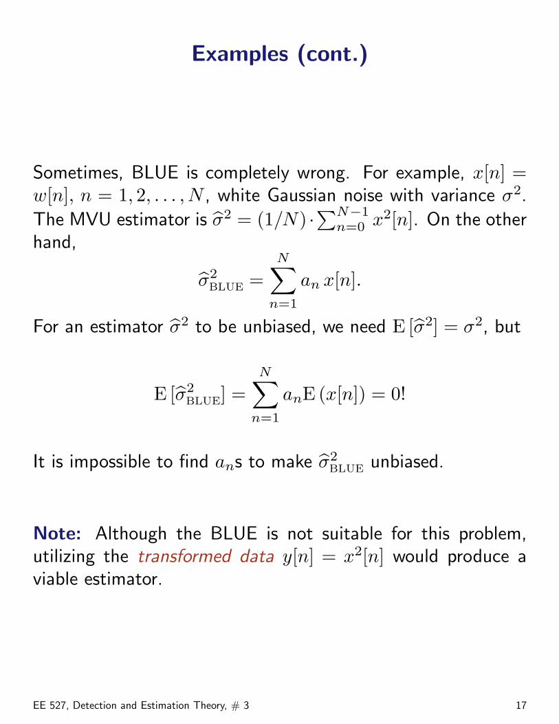
Examples (cont.)

Sometimes, BLUE is completely wrong. For example, x[n] =w[n], n = 1, 2, . . . , N , white Gaussian noise with variance σ2.

The MVU estimator is σ2 = (1/N) ·∑N−1

n=0 x2[n]. On the otherhand,

σ2BLUE =

N∑n=1

an x[n].

For an estimator σ2 to be unbiased, we need E [σ2] = σ2, but

E [σ2BLUE] =

N∑n=1

anE (x[n]) = 0!

It is impossible to find ans to make σ2BLUE unbiased.

Note: Although the BLUE is not suitable for this problem,utilizing the transformed data y[n] = x2[n] would produce aviable estimator.

EE 527, Detection and Estimation Theory, # 3 17

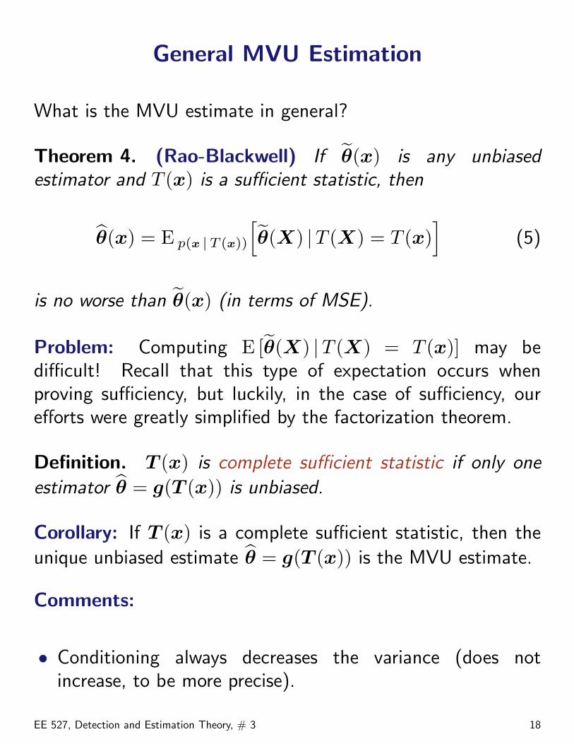
General MVU Estimation

What is the MVU estimate in general?

Theorem 4. (Rao-Blackwell) If θ(x) is any unbiasedestimator and T (x) is a sufficient statistic, then

θ(x) = E p(x |T (x))

[θ(X) |T (X) = T (x)

](5)

is no worse than θ(x) (in terms of MSE).

Problem: Computing E [θ(X) |T (X) = T (x)] may bedifficult! Recall that this type of expectation occurs whenproving sufficiency, but luckily, in the case of sufficiency, ourefforts were greatly simplified by the factorization theorem.

Definition. T (x) is complete sufficient statistic if only one

estimator θ = g(T (x)) is unbiased.

Corollary: If T (x) is a complete sufficient statistic, then the

unique unbiased estimate θ = g(T (x)) is the MVU estimate.

Comments:

• Conditioning always decreases the variance (does notincrease, to be more precise).

EE 527, Detection and Estimation Theory, # 3 18

• To get a realizable estimator, we need to condition on thesufficient statistics. The definition of sufficient statistic[denoted by T (x)] implies that conditioning on it leads to adistribution that is not a function of the unknown parametersθ. Hence, (5) is a statistic, i.e. realizable.

EE 527, Detection and Estimation Theory, # 3 19

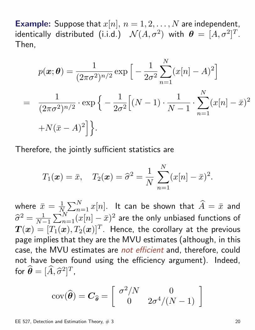
Example: Suppose that x[n], n = 1, 2, . . . , N are independent,identically distributed (i.i.d.) N (A, σ2) with θ = [A, σ2]T .Then,

p(x;θ) =1

(2πσ2)n/2exp

[− 1

2σ2

N∑n=1

(x[n]−A)2]

=1

(2πσ2)n/2· exp

{− 1

2σ2

[(N − 1) · 1

N − 1·

N∑n=1

(x[n]− x)2

+N(x−A)2]}

.

Therefore, the jointly sufficient statistics are

T1(x) = x, T2(x) = σ2 =1N

N∑n=1

(x[n]− x)2.

where x = 1N

∑Nn=1 x[n]. It can be shown that A = x and

σ2 = 1N−1

∑Nn=1(x[n]− x)2 are the only unbiased functions of

T (x) = [T1(x), T2(x)]T . Hence, the corollary at the previouspage implies that they are the MVU estimates (although, in thiscase, the MVU estimates are not efficient and, therefore, couldnot have been found using the efficiency argument). Indeed,

for θ = [A, σ2]T ,

cov(θ) = Cbθ =[

σ2/N 00 2σ4/(N − 1)

]EE 527, Detection and Estimation Theory, # 3 20

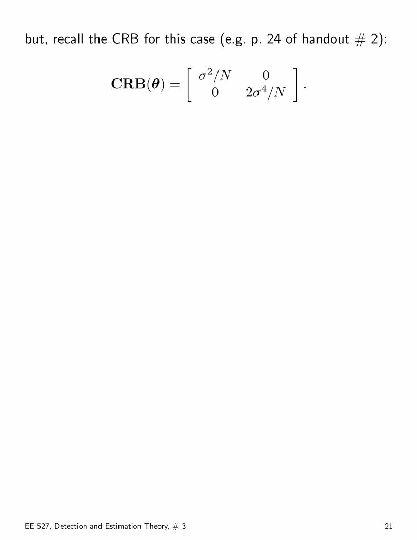
but, recall the CRB for this case (e.g. p. 24 of handout # 2):

CRB(θ) =[

σ2/N 00 2σ4/N

].

EE 527, Detection and Estimation Theory, # 3 21

MAXIMUM LIKELIHOOD (ML) ESTIMATION

θ = arg maxθ

p(x; θ).

The pdf p(x; θ), viewed as function of θ, is the likelihoodfunction.

Comments on the likelihood function: For given θ anddiscrete case, p(x; θ) is the probability of observing the pointx. In the continuous case, it is approximately proportional toprobability of observing a point in a small rectangle aroundx. However, when we think of p(x; θ) as a function of θ, itgives, for a given observed x, the “likelihood” or “plausibility”of various θ.

ML estimate ≡ value of the parameter θ that “makes theprobability of the data as great as it can be under the assumedmodel.”

EE 527, Detection and Estimation Theory, # 3 22

ML Estimation (cont.)

Theorem 5. Assume that certain regularity conditions holdand let θ be the ML estimate. Then, as N →∞,

θ → θ0 (with probability 1) (consistency) (6)√

N (θ − θ0)d→ N

(0, N I−1(θ0)

)(asymptotic efficiency) (7)

where θ0 is the true value of the parameter and I(θ0) is theFisher information [and I−1(θ0) the CRB]. Moreover, if anefficient (in finite samples) estimate exists, it is given by theML estimate.

Proof. See e.g. Rao, Chapter 5f.2 at pp. 364–366 for the caseof independent observations. 2

Note: At lower signal-to-noise ratios (SNRs), a thresholdeffect occurs — outliers give rise to increased variance (morethan predicted by the CRB). This behavior is characteristic ofpractically all nonlinear estimators.

Example: x[n] i.i.d. N (θ, σ2), n = 0, 1, . . . , N − 1, for σ2

EE 527, Detection and Estimation Theory, # 3 23

known. Maximizing p(x; θ) is equivalent to

maxθ

log p(x; θ) = const− 12σ2

N−1∑n=0

(x[n]− θ)2.

Thus, the ML estimate is the sample mean

θ =1N

N−1∑n=0

x[n] ∼ N (θ0, σ2/N).

In this example, ML estimator = MVU estimator = BLUE.

Note: When estimation error cannot be made small as N →∞, the asymptotic pdf in (7) is invalid. For asymptotics towork, there has to be an averaging effect!

Example 7.7 in Kay-I: Estimation of the DC level in fullydependent non-Gaussian noise:

x[n] = A + w[n].

We observe x[0], x[1], . . . , x[N − 1] but w[0] = w[1] = · · · =w[N−1], i.e. all noise samples are the same. Hence, we discard

x[1], x[2], . . . , x[N − 1]. Then, A = x[0], say. The pdf of A

remains non-Gaussian as N → ∞. Also, A is not consistentsince var(A) = var(x[0]) 9 0 as N →∞.

EE 527, Detection and Estimation Theory, # 3 24

ML Estimation: Vector Parameters

Nothing really changes. The ML estimate is

θ = arg maxθ

p(x;θ).

Under appropriate regularity conditions, this estimate isconsistent and

√N (θ − θ0)

d→ N(0, N I−1(θ0)

)where I(θ0) is the Fisher information matrix now.

EE 527, Detection and Estimation Theory, # 3 25

ML Estimation: Properties

Theorem 6. (ML Invariance Principle) The ML estimateof α = g(θ) where the pdf/pmf p(x;θ) is parametrized by θ,is given by

α = g(θ)

where θ is the ML estimate of θ [obtained by maximizingp(x;θ) with respect to θ].

Comments:

• For a more precise formulation, see Theorems 7.2 and 7.4 inKay-I.

• Invariance is often combined with the delta method whichwe introduce later in this handout.

More properties:

• If a given scalar parameter θ has a single sufficient statisticT (x), say, then the ML estimate of θ must be a function ofT (x). Furthermore, if T (x) is minimal and complete, thenthe ML estimate is unique.

• (Connection between ML and MVU estimation) If theML estimate is unbiased, then it is MVU.

EE 527, Detection and Estimation Theory, # 3 26

Statistical Motivation

ML has a nice intuitive interpretation, but is it justifiablestatistically? Now we try to add to the answer to this question,focusing on the case of i.i.d. observations.

In Ch. 6.2 of Theory of Point Estimation, Lehmann shows thefollowing result.

Theorem 7. Suppose that the random observations Xi arei.i.d. with common pdf/pmf p(xi;θ0) where θ0 is in the interiorof the parameter space. Then, as N →∞

P{ N∏

i=1

p(Xi;θ0) >

N∏i=1

p(Xi;θ)}→ 1

for any fixed θ 6= θ0.

Comment: This theorem states that, for large number of i.i.d.samples (i.e. large N), the joint pdf/pmf of X1, X2, . . . , XN atthe true parameter value

N∏i=1

p(Xi;θ0)

exceeds the joint pdf/pmf of X1, X2, . . . , XN at any otherparameter value (with probability one). Consequently, as the

EE 527, Detection and Estimation Theory, # 3 27

number of observations increases, the parameter estimate thatmaximizes the joint distribution of the measurements (i.e. theML estimate) must become close to the true value.

EE 527, Detection and Estimation Theory, # 3 28

Regularity Conditions for I.I.D. Observations

Not one set of regularity conditions applies to all scenarios.

Here are some typical regularity conditions for the i.i.d. case.Suppose X1, . . . , Xn are i.i.d. with pdf

p(xi;θ), θ =

θ1

θ2...θp

.

Regularity conditions:

(i) p(x;θ) is identifiable for θ and the support of p(xi;θ) isnot a function of θ;

(ii) The true value of the parameter, say θ0, lies in an opensubset of the parameter space Θ;

(iii) For almost all x, the pdf p(x;θ) has continuous derivativesto order three with respect to all elements of θ and all valuesin the open subset of (ii);

(iv) The following are satisfied:

E p(x;θ)

[ ∂

∂θklog p(X;θ)

]= 0, k = 1, 2, . . . , p

EE 527, Detection and Estimation Theory, # 3 29

and

Ii,k(θ) = E p(x;θ)

[∂

∂θilog p(X;θ) · ∂

∂θklog p(X;θ)

]= −E

[∂2

∂θi ∂θklog p(X;θ)

], i, k = 1, 2, . . . , p.

(v) The FIM I(θ) = [I(θ)]i,k is positive definite;

(vi) Bounding functions mi,k,l(·) exist such that

∣∣∣ ∂3

∂θi ∂θk ∂θllog p(x;θ)

∣∣∣ ≤ mi,k,l(x)

for all θ in the open subset of (ii), and

E p(x;θ)[mi,k,l(X)] < ∞.

Theorem 8. (≈ same as Theorem 5) If X1, X2, . . . , XN

are i.i.d. with pdf p(xi;θ) such that the conditions (i)–(vi)

hold, then there exists a sequence of solutions {θN} to thelikelihood equations such that

(i) θN is consistent for θ;

(ii)√

N (θN − θ) is asymptotically Gaussian with mean 0 andcovariance matrix N I−1(θ) = N CRB(θ);

EE 527, Detection and Estimation Theory, # 3 30

(iii)√

N ([θN ]i − θi) is asymptotically Gaussian with mean 0and variance N [I−1(θ)]i,i, i = 1, 2, . . . , p.

Comments: What we are not given:

(i) uniqueness of θN ;

(ii) existence for all x1, . . . , xN ;

(iii) even if the solution exists and is unique, that we can findit.

EE 527, Detection and Estimation Theory, # 3 31

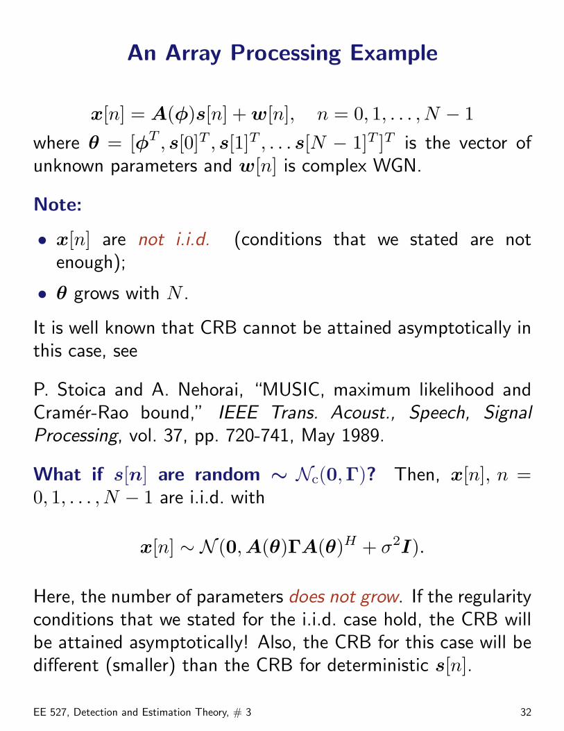
An Array Processing Example

x[n] = A(φ)s[n] + w[n], n = 0, 1, . . . , N − 1where θ = [φT , s[0]T , s[1]T , . . . s[N − 1]T ]T is the vector ofunknown parameters and w[n] is complex WGN.

Note:

• x[n] are not i.i.d. (conditions that we stated are notenough);

• θ grows with N .

It is well known that CRB cannot be attained asymptotically inthis case, see

P. Stoica and A. Nehorai, “MUSIC, maximum likelihood andCramer-Rao bound,” IEEE Trans. Acoust., Speech, SignalProcessing, vol. 37, pp. 720-741, May 1989.

What if s[n] are random ∼ Nc(0,Γ)? Then, x[n], n =0, 1, . . . , N − 1 are i.i.d. with

x[n] ∼ N (0,A(θ)ΓA(θ)H + σ2I).

Here, the number of parameters does not grow. If the regularityconditions that we stated for the i.i.d. case hold, the CRB willbe attained asymptotically! Also, the CRB for this case will bedifferent (smaller) than the CRB for deterministic s[n].

EE 527, Detection and Estimation Theory, # 3 32

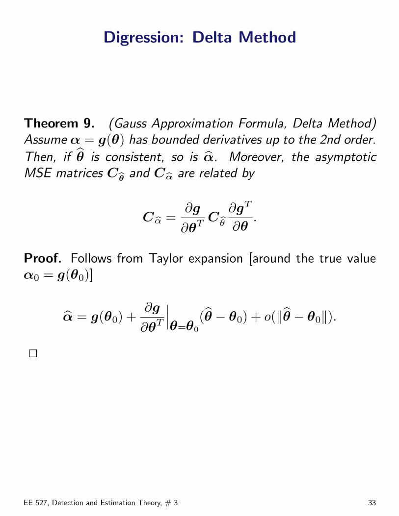
Digression: Delta Method

Theorem 9. (Gauss Approximation Formula, Delta Method)Assume α = g(θ) has bounded derivatives up to the 2nd order.

Then, if θ is consistent, so is α. Moreover, the asymptoticMSE matrices Cbθ and Cbα are related by

Cbα =∂g

∂θTCbθ ∂gT

∂θ.

Proof. Follows from Taylor expansion [around the true valueα0 = g(θ0)]

α = g(θ0) +∂g

∂θT

∣∣∣θ=θ0

(θ − θ0) + o(‖θ − θ0‖).

2

EE 527, Detection and Estimation Theory, # 3 33

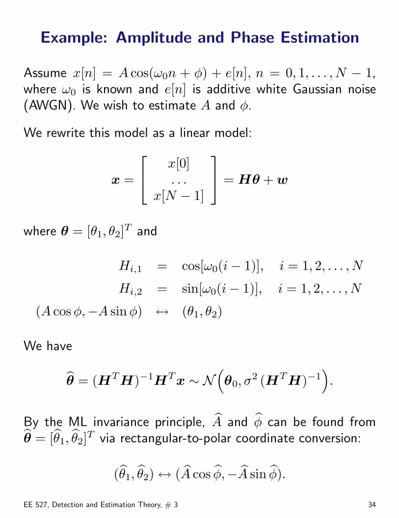
Example: Amplitude and Phase Estimation

Assume x[n] = A cos(ω0n + φ) + e[n], n = 0, 1, . . . , N − 1,where ω0 is known and e[n] is additive white Gaussian noise(AWGN). We wish to estimate A and φ.

We rewrite this model as a linear model:

x =

x[0]. . .

x[N − 1]

= Hθ + w

where θ = [θ1, θ2]T and

Hi,1 = cos[ω0(i− 1)], i = 1, 2, . . . , N

Hi,2 = sin[ω0(i− 1)], i = 1, 2, . . . , N

(A cos φ,−A sinφ) ↔ (θ1, θ2)

We have

θ = (HTH)−1HTx ∼ N(θ0, σ

2 (HTH)−1).

By the ML invariance principle, A and φ can be found fromθ = [θ1, θ2]T via rectangular-to-polar coordinate conversion:

(θ1, θ2) ↔ (A cos φ,−A sin φ).

EE 527, Detection and Estimation Theory, # 3 34

Define α = [A,φ]T = g(θ). Then, the delta method yields

Cbα =∂g

∂θTCbθ ∂gT

∂θ.

EE 527, Detection and Estimation Theory, # 3 35

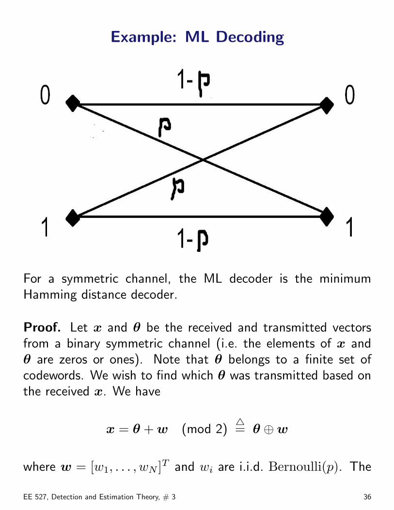
Example: ML Decoding

For a symmetric channel, the ML decoder is the minimumHamming distance decoder.

Proof. Let x and θ be the received and transmitted vectorsfrom a binary symmetric channel (i.e. the elements of x andθ are zeros or ones). Note that θ belongs to a finite set ofcodewords. We wish to find which θ was transmitted based onthe received x. We have

x = θ + w (mod 2)4= θ ⊕w

where w = [w1, . . . , wN ]T and wi are i.i.d. Bernoulli(p). The

EE 527, Detection and Estimation Theory, # 3 36

likelihood function is given by

p(x;θ) = P{X = x} = P{θ ⊕ W︸︷︷︸i.i.d. Bernoulli

= x}

= P{W = x⊕ θ︸ ︷︷ ︸w=

2666664w1

w2...

wN

3777775

}

= pPN

i=1 wi · (1− p)N−PN

i=1 wi

=(

p

1− p

)dH(x,θ)

(1− p)N

where

dH(x,θ) =N∑

i=1

xi ⊕ θi

is the Hamming distance between x and θ (i.e. the numberof bits that are different between the two vectors). Hence, ifp < 0.5, then

maxx

p(x;θ) ⇐⇒ minθ

dH(x,θ).

2

EE 527, Detection and Estimation Theory, # 3 37

Asymptotic ML for WSS Processes

Consider data x ∼ N (0,C(θ)). To find the ML estimate ofθ, maximize

p(x;θ) =1

(2π)N/2|C(θ)|1/2exp

[− 1

2 · xTC(θ)−1

x]

over θ.

If x[n] is WSS, then C(θ) is Toplitz, so, as N → ∞, we canapproximate the log likelihood as:

log p(x; θ) = −N

2log 2π

−N

2

∫ 1/2

−1/2

(log Pxx(f ;θ) +

Ix(f)Pxx(f ;θ)

)df

where Ix(f) is the periodogram:

Ix(f) =1N

∣∣∣ N−1∑n=0

x[n]e−j2πfn∣∣∣2

and Pxx(f ; θ) is the PSD of x[n].

This result is based on the Whittle approximation, see e.g.

P. Whittle, “The analysis of multiple stationary time series,” J.R. Stat. Soc., Ser. B vol. 15, pp. 125–139, 1953.

EE 527, Detection and Estimation Theory, # 3 38

Proof. See e.g. Ch. 7.9 in Kay-I. 2

Note: Kay calls the Whittle approximation “asymptotic ML”.

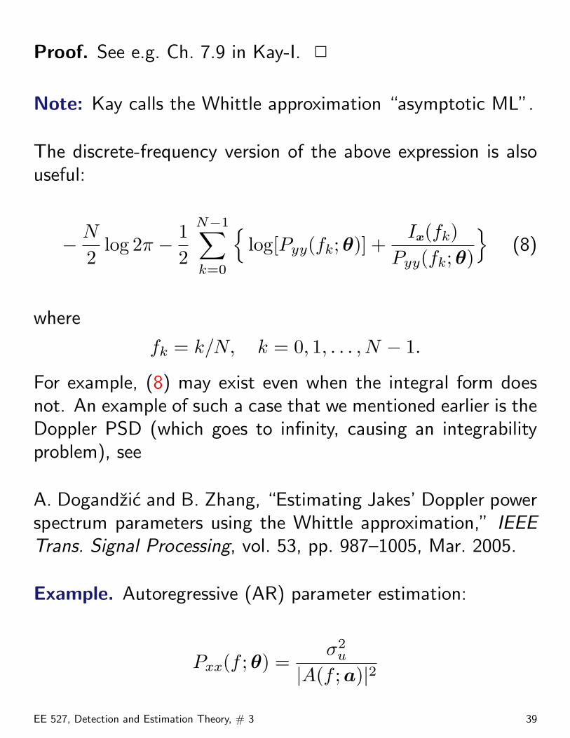
The discrete-frequency version of the above expression is alsouseful:

− N

2log 2π − 1

2

N−1∑k=0

{log[Pyy(fk;θ)] +

Ix(fk)Pyy(fk;θ)

}(8)

where

fk = k/N, k = 0, 1, . . . , N − 1.

For example, (8) may exist even when the integral form doesnot. An example of such a case that we mentioned earlier is theDoppler PSD (which goes to infinity, causing an integrabilityproblem), see

A. Dogandzic and B. Zhang, “Estimating Jakes’ Doppler powerspectrum parameters using the Whittle approximation,” IEEETrans. Signal Processing, vol. 53, pp. 987–1005, Mar. 2005.

Example. Autoregressive (AR) parameter estimation:

Pxx(f ;θ) =σ2

u

|A(f ;a)|2

EE 527, Detection and Estimation Theory, # 3 39

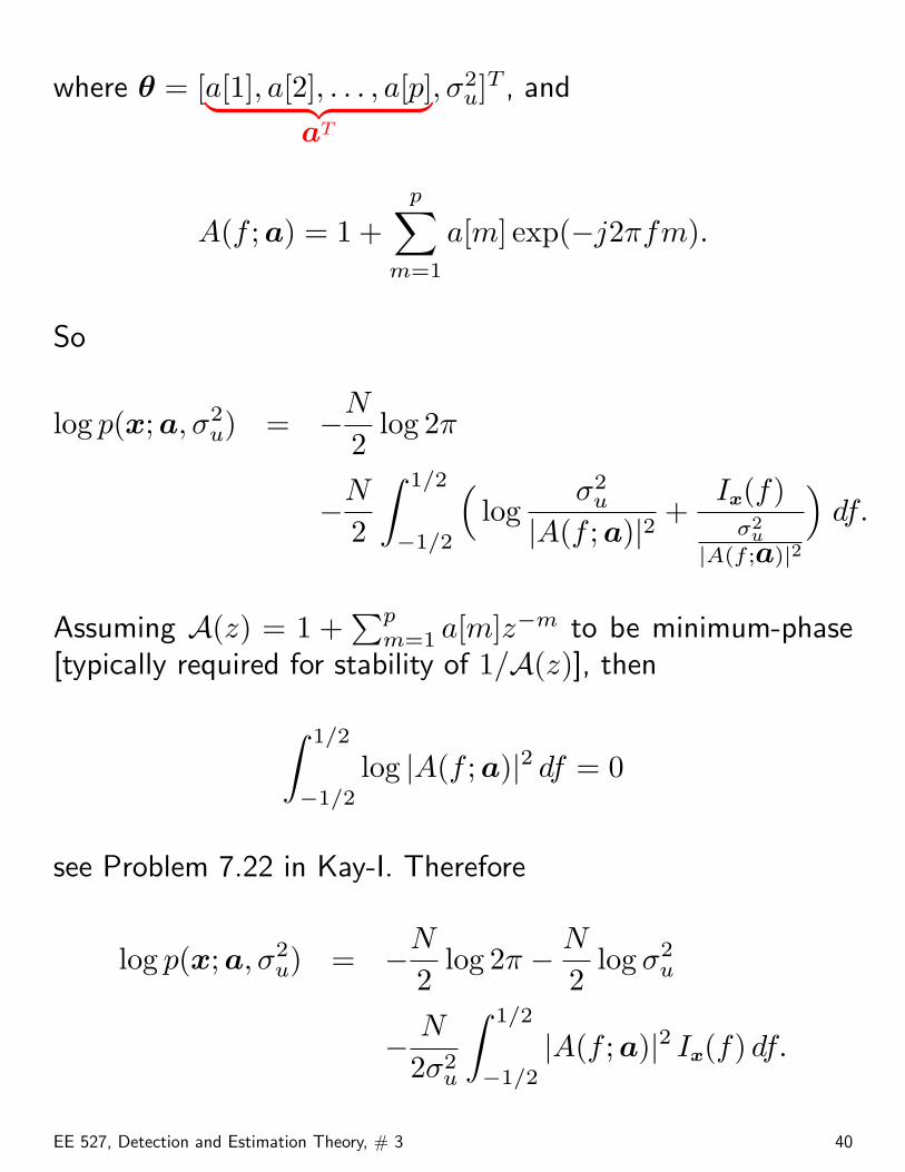
where θ = [a[1], a[2], . . . , a[p]︸ ︷︷ ︸aT

, σ2u]T , and

A(f ;a) = 1 +p∑

m=1

a[m] exp(−j2πfm).

So

log p(x;a, σ2u) = −N

2log 2π

−N

2

∫ 1/2

−1/2

(log

σ2u

|A(f ;a)|2+

Ix(f)σ2

u|A(f ;a)|2

)df.

Assuming A(z) = 1 +∑p

m=1 a[m]z−m to be minimum-phase[typically required for stability of 1/A(z)], then

∫ 1/2

−1/2

log |A(f ;a)|2 df = 0

see Problem 7.22 in Kay-I. Therefore

log p(x;a, σ2u) = −N

2log 2π − N

2log σ2

u

− N

2σ2u

∫ 1/2

−1/2

|A(f ;a)|2 Ix(f) df.

EE 527, Detection and Estimation Theory, # 3 40

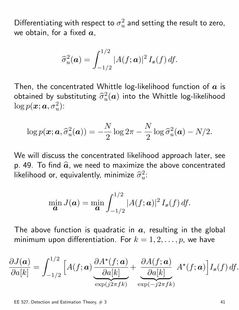
Differentiating with respect to σ2u and setting the result to zero,

we obtain, for a fixed a,

σ2u(a) =

∫ 1/2

−1/2

|A(f ;a)|2 Ix(f) df.

Then, the concentrated Whittle log-likelihood function of a isobtained by substituting σ2

u(a) into the Whittle log-likelihoodlog p(x;a, σ2

u):

log p(x;a, σ2u(a)) = −N

2log 2π − N

2log σ2

u(a)−N/2.

We will discuss the concentrated likelihood approach later, seep. 49. To find a, we need to maximize the above concentratedlikelihood or, equivalently, minimize σ2

u:

mina

J(a) = mina

∫ 1/2

−1/2

|A(f ;a)|2 Ix(f) df.

The above function is quadratic in a, resulting in the globalminimum upon differentiation. For k = 1, 2, . . . , p, we have

∂J(a)∂a[k]

=∫ 1/2

−1/2

[A(f ;a)

∂A?(f ;a)∂a[k]︸ ︷︷ ︸

exp(j2πfk)

+∂A(f ;a)

∂a[k]︸ ︷︷ ︸exp(−j2πfk)

A?(f ;a)]Ix(f) df.

EE 527, Detection and Estimation Theory, # 3 41

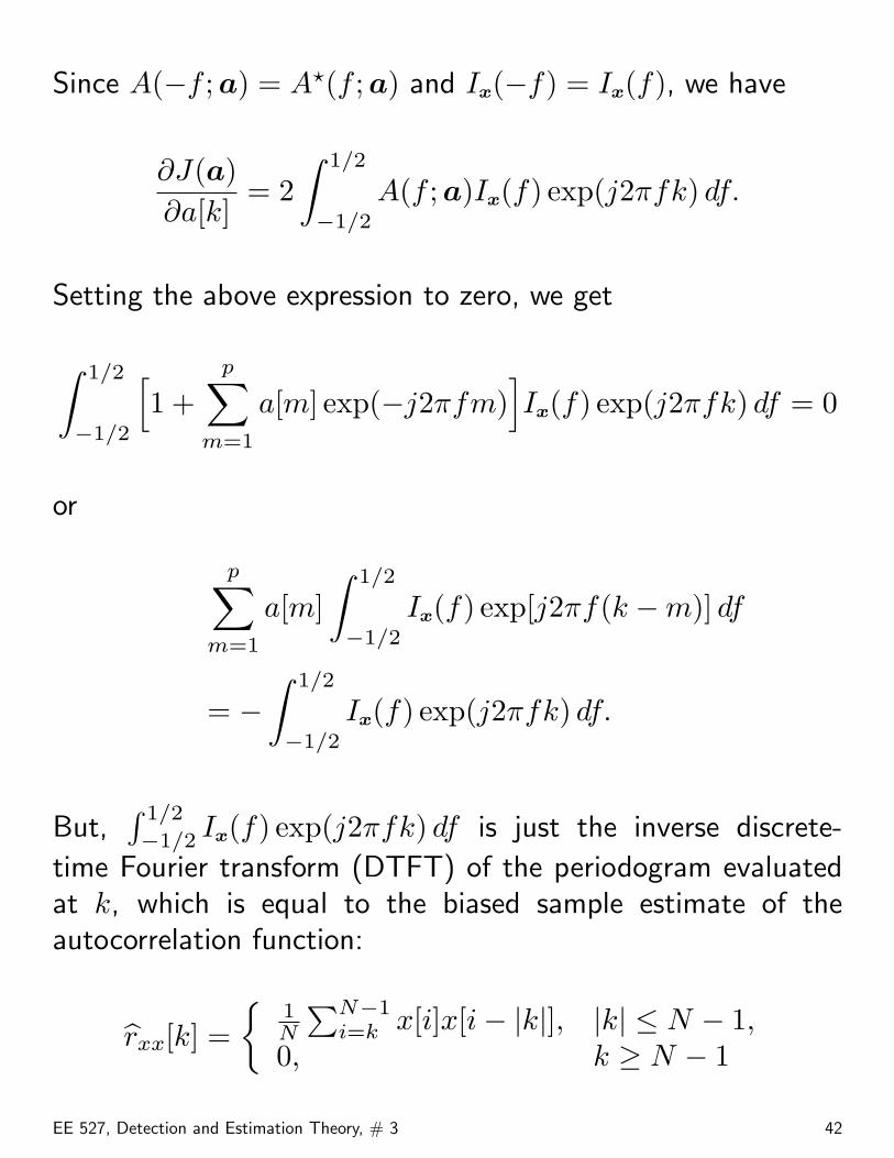
Since A(−f ;a) = A?(f ;a) and Ix(−f) = Ix(f), we have

∂J(a)∂a[k]

= 2∫ 1/2

−1/2

A(f ;a)Ix(f) exp(j2πfk) df.

Setting the above expression to zero, we get

∫ 1/2

−1/2

[1 +

p∑m=1

a[m] exp(−j2πfm)]Ix(f) exp(j2πfk) df = 0

or

p∑m=1

a[m]∫ 1/2

−1/2

Ix(f) exp[j2πf(k −m)] df

= −∫ 1/2

−1/2

Ix(f) exp(j2πfk) df.

But,∫ 1/2

−1/2Ix(f) exp(j2πfk) df is just the inverse discrete-

time Fourier transform (DTFT) of the periodogram evaluatedat k, which is equal to the biased sample estimate of theautocorrelation function:

rxx[k] ={

1N

∑N−1i=k x[i]x[i− |k|], |k| ≤ N − 1,

0, k ≥ N − 1

EE 527, Detection and Estimation Theory, # 3 42

Hence, the Whittle (asymptotic) ML estimate of the AR filterparameter vector a solves

p∑m=1

a[m] rxx[k −m] = −rxx[k], k = 1, 2, . . . , p

which are the estimated Yule-Walker equations.

EE 527, Detection and Estimation Theory, # 3 43

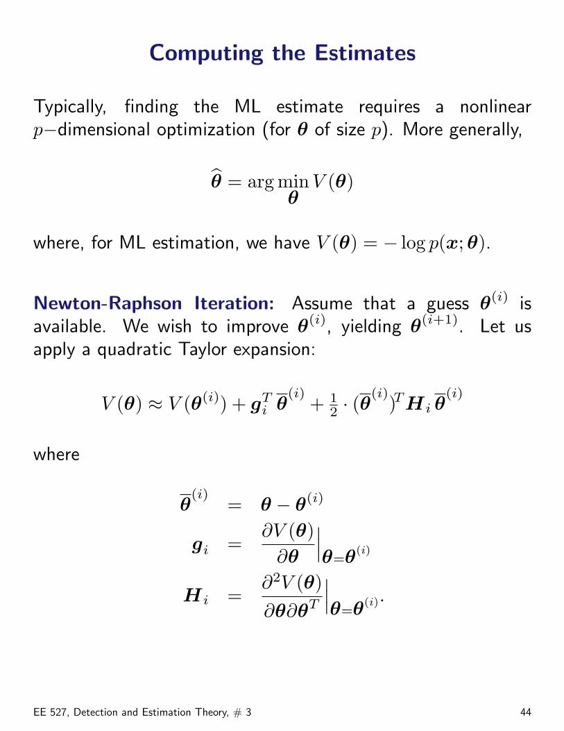
Computing the Estimates

Typically, finding the ML estimate requires a nonlinearp−dimensional optimization (for θ of size p). More generally,

θ = arg minθ

V (θ)

where, for ML estimation, we have V (θ) = − log p(x;θ).

Newton-Raphson Iteration: Assume that a guess θ(i) isavailable. We wish to improve θ(i), yielding θ(i+1). Let usapply a quadratic Taylor expansion:

V (θ) ≈ V (θ(i)) + gTi θ

(i)+ 1

2 · (θ(i)

)THi θ(i)

where

θ(i)

= θ − θ(i)

gi =∂V (θ)

∂θ

∣∣∣θ=θ(i)

Hi =∂2V (θ)∂θ∂θT

∣∣∣θ=θ(i).

EE 527, Detection and Estimation Theory, # 3 44

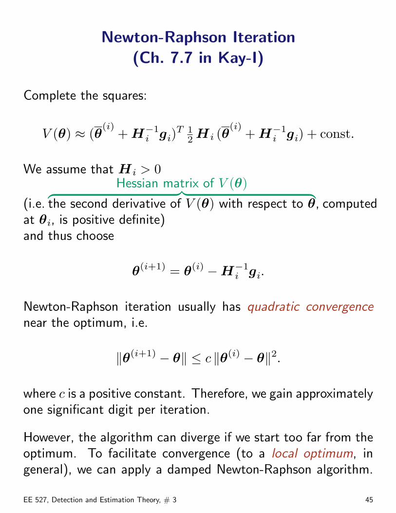
Newton-Raphson Iteration(Ch. 7.7 in Kay-I)

Complete the squares:

V (θ) ≈ (θ(i)

+ H−1i gi)

T 12 Hi (θ

(i)+ H−1

i gi) + const.

We assume that Hi > 0

(i.e.

Hessian matrix of V (θ)︷ ︸︸ ︷the second derivative of V (θ) with respect to θ, computed

at θi, is positive definite)and thus choose

θ(i+1) = θ(i) −H−1i gi.

Newton-Raphson iteration usually has quadratic convergencenear the optimum, i.e.

‖θ(i+1) − θ‖ ≤ c ‖θ(i) − θ‖2.

where c is a positive constant. Therefore, we gain approximatelyone significant digit per iteration.

However, the algorithm can diverge if we start too far from theoptimum. To facilitate convergence (to a local optimum, ingeneral), we can apply a damped Newton-Raphson algorithm.

EE 527, Detection and Estimation Theory, # 3 45

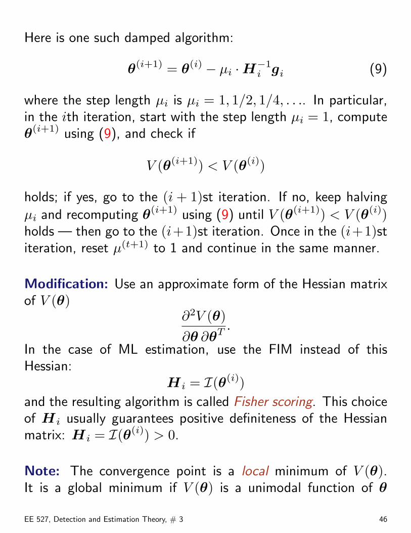
Here is one such damped algorithm:

θ(i+1) = θ(i) − µi ·H−1i gi (9)

where the step length µi is µi = 1, 1/2, 1/4, . . .. In particular,in the ith iteration, start with the step length µi = 1, computeθ(i+1) using (9), and check if

V (θ(i+1)) < V (θ(i))

holds; if yes, go to the (i + 1)st iteration. If no, keep halving

µi and recomputing θ(i+1) using (9) until V (θ(i+1)) < V (θ(i))holds — then go to the (i+1)st iteration. Once in the (i+1)stiteration, reset µ(t+1) to 1 and continue in the same manner.

Modification: Use an approximate form of the Hessian matrixof V (θ)

∂2V (θ)∂θ ∂θT

.

In the case of ML estimation, use the FIM instead of thisHessian:

Hi = I(θ(i))and the resulting algorithm is called Fisher scoring. This choiceof Hi usually guarantees positive definiteness of the Hessianmatrix: Hi = I(θ(i)) > 0.

Note: The convergence point is a local minimum of V (θ).It is a global minimum if V (θ) is a unimodal function of θ

EE 527, Detection and Estimation Theory, # 3 46

or if the initial estimate is sufficiently good. (If we suspectthat) there are multiple local minima of V (θ) (i.e. multiplelocal maxima of the likelihood function), we should try many(wide-spread/different) starting values for our Newton-Raphsonor Fisher scoring iterations.

If the parameter space Θ is not RI p, we should also examine theboundary of the parameter space to see if a global maximumof the likelihood function (i.e. a global minimum of V (θ))lies on this boundary. Pay attention to this issue in yourhomework assignments and exams, as well as in general.

EE 527, Detection and Estimation Theory, # 3 47

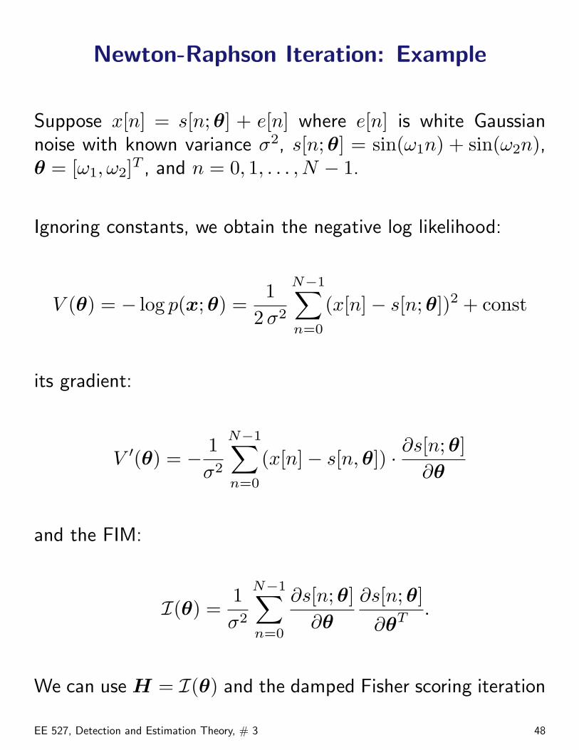
Newton-Raphson Iteration: Example

Suppose x[n] = s[n;θ] + e[n] where e[n] is white Gaussiannoise with known variance σ2, s[n;θ] = sin(ω1n) + sin(ω2n),θ = [ω1, ω2]T , and n = 0, 1, . . . , N − 1.

Ignoring constants, we obtain the negative log likelihood:

V (θ) = − log p(x;θ) =1

2 σ2

N−1∑n=0

(x[n]− s[n;θ])2 + const

its gradient:

V ′(θ) = − 1σ2

N−1∑n=0

(x[n]− s[n, θ]) · ∂s[n;θ]∂θ

and the FIM:

I(θ) =1σ2

N−1∑n=0

∂s[n;θ]∂θ

∂s[n;θ]∂θT

.

We can use H = I(θ) and the damped Fisher scoring iteration

EE 527, Detection and Estimation Theory, # 3 48

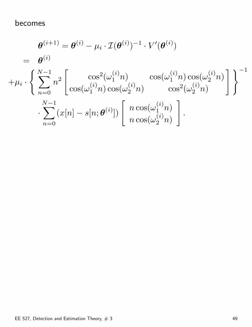
becomes

θ(i+1) = θ(i) − µi · I(θ(i))−1 · V ′(θ(i))

= θ(i)

+µi ·

{N−1∑n=0

n2

[cos2(ω(i)

1 n) cos(ω(i)1 n) cos(ω(i)

2 n)cos(ω(i)

1 n) cos(ω(i)2 n) cos2(ω(i)

2 n)

] }−1

·N−1∑n=0

(x[n]− s[n;θ(i)])

[n cos(ω(i)

1 n)n cos(ω(i)

2 n)

].

EE 527, Detection and Estimation Theory, # 3 49

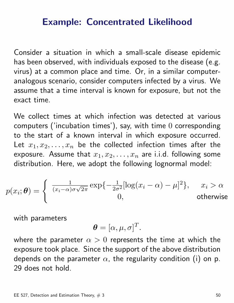
Example: Concentrated Likelihood

Consider a situation in which a small-scale disease epidemichas been observed, with individuals exposed to the disease (e.g.virus) at a common place and time. Or, in a similar computer-analogous scenario, consider computers infected by a virus. Weassume that a time interval is known for exposure, but not theexact time.

We collect times at which infection was detected at variouscomputers (’incubation times’), say, with time 0 correspondingto the start of a known interval in which exposure occurred.Let x1, x2, . . . , xn be the collected infection times after theexposure. Assume that x1, x2, . . . , xn are i.i.d. following somedistribution. Here, we adopt the following lognormal model:

p(xi;θ) =

{1

(xi−α)σ√

2πexp{− 1

2σ2[log(xi − α)− µ]2}, xi > α

0, otherwise

with parametersθ = [α, µ, σ]T .

where the parameter α > 0 represents the time at which theexposure took place. Since the support of the above distributiondepends on the parameter α, the regularity condition (i) on p.29 does not hold.

EE 527, Detection and Estimation Theory, # 3 50

Here are some references related to the above model:

H.L. Harter and A.H. Moore, “Local-maximum-likelihoodestimation of the parameters of three-parameter lognormalpopulations from complete and censored samples,” J. Amer.Stat. Assoc., vol. 61, pp. 842–851, Sept. 1966.

B.M. Hill, “The three-parameter lognormal distribution andBayesian analysis of a point-source epidemic,” J. Amer. Stat.Assoc., vol. 68, pp. 72–84, Mar. 1963.

Note: this model is equivalent to having xi, i = 1, 2, . . . , Nsuch that log(xi − α) ∼ N (µ, σ2).

The log-likelihood function is

l(θ) =N∑

i=1

log p(xi;θ)

= −N

2log(2πσ2)−

N∑i=1

log(xi − α)

− 12σ2

N∑i=1

[log(xi − α)− µ

]2where xi > α, ∀i = 1, 2, . . . , N .

For a fixed α, we can easily find µ and σ2 that maximize the

EE 527, Detection and Estimation Theory, # 3 51

likelihood:

µ(α) =1N

N∑t=1

log(xi − α)

σ2(α) =1N

N∑t=1

[log(xi − α)− µ(α)]2

which follows from the above relationship with the normal pdf.Now, we can write the log-likelihood function as a function ofα alone, by substituting µ(α) and σ2(α) into l(θ):

l([α, µ(α), σ2(α)]T )

= −N

2log[2πσ2(α)]−

N∑i=1

log(xi − α)− N

2.

EE 527, Detection and Estimation Theory, # 3 52

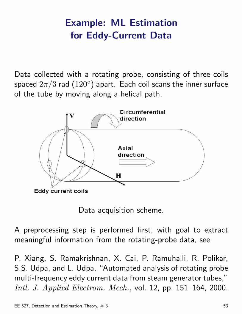
Example: ML Estimationfor Eddy-Current Data

Data collected with a rotating probe, consisting of three coilsspaced 2π/3 rad (120◦) apart. Each coil scans the inner surfaceof the tube by moving along a helical path.

Data acquisition scheme.

A preprocessing step is performed first, with goal to extractmeaningful information from the rotating-probe data, see

P. Xiang, S. Ramakrishnan, X. Cai, P. Ramuhalli, R. Polikar,S.S. Udpa, and L. Udpa, “Automated analysis of rotating probemulti-frequency eddy current data from steam generator tubes,”Intl. J. Applied Electrom. Mech., vol. 12, pp. 151–164, 2000.

EE 527, Detection and Estimation Theory, # 3 53

−200 0 200 600

0.5

1

1.5

2

2.5x 10

4

(a)

1−D signal 2−D image

(b)20 60 100

50

100

150

200

−200

−100

0

100

200

300

400

500

600

image after preprocessing

(c)20 60 100

50

100

150

200

−0.5

0

0.5

1

1.5

2

2.5

3

3.5

4

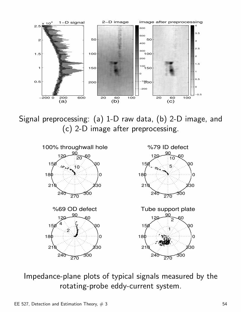
Signal preprocessing: (a) 1-D raw data, (b) 2-D image, and(c) 2-D image after preprocessing.

10

2030

210

60

240

90

270

120

300

150

330

180 0

100% throughwall hole

5

1030

210

60

240

90

270

120

300

150

330

180 0

%79 ID defect

2

4 30

210

60

240

90

270

120

300

150

330

180 0

%69 OD defect

1

230

210

60

240

90

270

120

300

150

330

180 0

Tube support plate

Impedance-plane plots of typical signals measured by therotating-probe eddy-current system.

EE 527, Detection and Estimation Theory, # 3 54

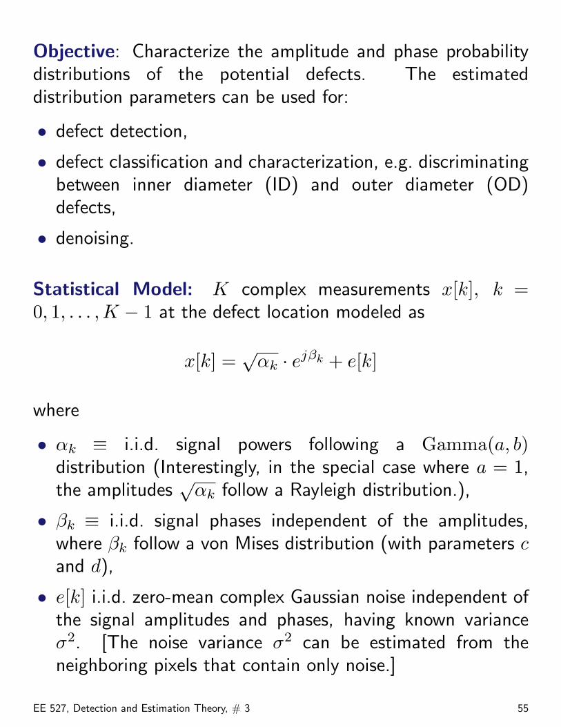
Objective: Characterize the amplitude and phase probabilitydistributions of the potential defects. The estimateddistribution parameters can be used for:

• defect detection,

• defect classification and characterization, e.g. discriminatingbetween inner diameter (ID) and outer diameter (OD)defects,

• denoising.

Statistical Model: K complex measurements x[k], k =0, 1, . . . ,K − 1 at the defect location modeled as

x[k] =√

αk · ejβk + e[k]

where

• αk ≡ i.i.d. signal powers following a Gamma(a, b)distribution (Interestingly, in the special case where a = 1,the amplitudes

√αk follow a Rayleigh distribution.),

• βk ≡ i.i.d. signal phases independent of the amplitudes,where βk follow a von Mises distribution (with parameters cand d),

• e[k] i.i.d. zero-mean complex Gaussian noise independent ofthe signal amplitudes and phases, having known varianceσ2. [The noise variance σ2 can be estimated from theneighboring pixels that contain only noise.]

EE 527, Detection and Estimation Theory, # 3 55

0 5 100

0.1

0.2

0.3

0.4

0.5

0.6

0.7

0.8

0.9

1

α

p α(α;a

,b)

(a,b) = (1,0.5)

(1,1)

(2,2)(100,15)

0 2 4 6

0.5

1

1.5

2

2.5

3

3.5

4

4.5

5

5.5

β

p β(β;c,

d)

(c,d) = (0.3,23)

(2.8,200)

(5.0,80)

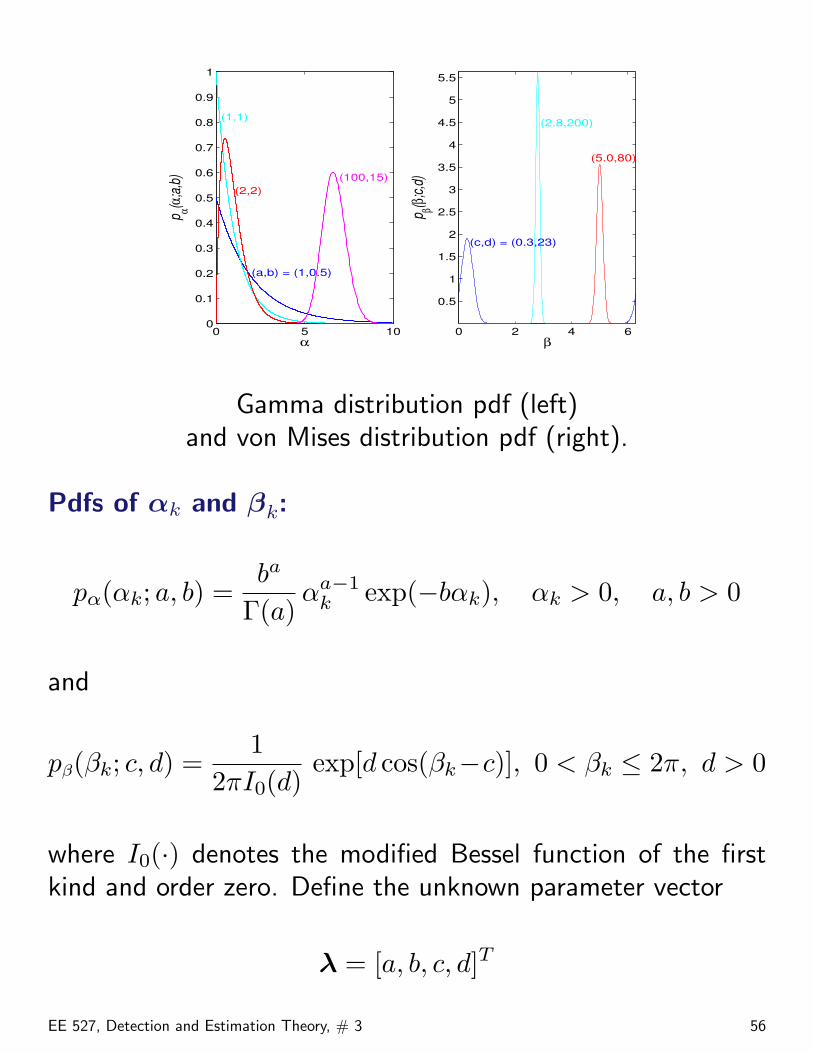
Gamma distribution pdf (left)and von Mises distribution pdf (right).

Pdfs of αk and βk:

pα(αk; a, b) =ba

Γ(a)αa−1

k exp(−bαk), αk > 0, a, b > 0

and

pβ(βk; c, d) =1

2πI0(d)exp[d cos(βk−c)], 0 < βk ≤ 2π, d > 0

where I0(·) denotes the modified Bessel function of the firstkind and order zero. Define the unknown parameter vector

λ = [a, b, c, d]T

EE 527, Detection and Estimation Theory, # 3 56

and the vectors of signal amplitudes and phases

θk = [αk, βk]T , k = 0, 1, . . . ,K − 1.

Marginal distribution of the kth observation:

px(x[k];λ) =∫Θ

px|θ(x[k] |θ) pθ(θ ; λ) dθ, k = 0, 1, . . . ,K − 1

where θ = [α, β]T , Θ = {(α, β) : 0 < α < ∞, 0 < β < 2π},and

px|θ(x[k] |θ) =1

πσ2exp

[− |x[k]−

√α · ejβ|2

σ2

]pθ(θ;λ) = pα(α; a, b) pβ(β; c, d).

ML estimate of λ obtained by maximizing the log-likelihood ofλ for all measurements x = [x[0], x[1], . . . , x[K − 1]]T :

L(λ,y) =K−1∑k=0

log px(x[k];λ). (10)

Newton-Raphson iteration for finding the ML estimates of λ[i.e. maximizing (10)]:

λ(i+1) = λ(i)−δ(i) ·[ ∂2L(λ(i))

∂λ ∂λT︸ ︷︷ ︸Hessian of the log likelihood

]−1 ∂L(λ(i))∂λ︸ ︷︷ ︸

gradient

(11)

EE 527, Detection and Estimation Theory, # 3 57

where the damping factor 0 < δ(i) ≤ 1 is chosen (at every stepi) to ensure that the likelihood function (10) increases and theparameter estimates remain in the allowable parameter space(a, b, d > 0).

We utilized the following formulas to compute the gradientvector and Hessian matrix in (11):

∂

∂λi{log px(x;λ)} =

1px(x;λ)

∫Θ

px|θ(x|θ)∂pθ(θ;λ)

∂λidθ

∂2

∂λi∂λm{log px(x;λ)} =

1px(x;λ)

∫Θ

px|θ(x|θ)∂2pθ(θ;λ)∂λi∂λm

dθ

− 1[px(x;λ)]2

·∫Θ

px|θ(x|θ)∂pθ(θ;λ)

∂λidθ ·

∫Θ

px|θ(x|θ)∂pθ(θ;λ)

∂λmdθ

for i,m = 1, 2, 3, 4.

The above integrals with respect to θ can be easily computedusing Gauss quadratures.

For more details, see

A. Dogandzic and P. Xiang, “A statistical model for eddy-current defect signals from steam generator tubes,” inRev. Progress Quantitative Nondestructive Evaluation, D.O.

EE 527, Detection and Estimation Theory, # 3 58

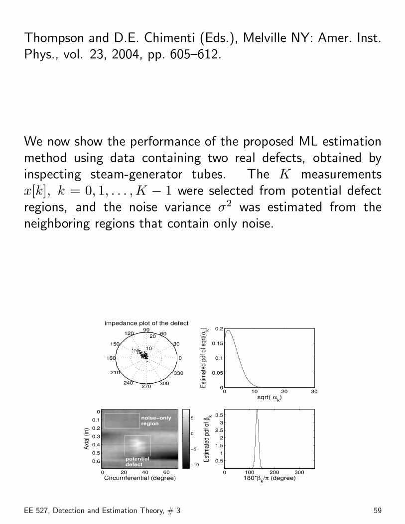
Thompson and D.E. Chimenti (Eds.), Melville NY: Amer. Inst.Phys., vol. 23, 2004, pp. 605–612.

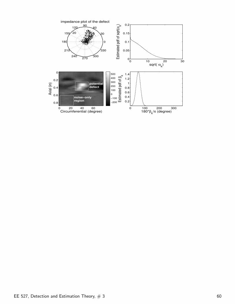
We now show the performance of the proposed ML estimationmethod using data containing two real defects, obtained byinspecting steam-generator tubes. The K measurementsx[k], k = 0, 1, . . . ,K − 1 were selected from potential defectregions, and the noise variance σ2 was estimated from theneighboring regions that contain only noise.

10

20

30

210

60

240

90

270

120

300

150

330

180 0

impedance plot of the defect

Circumferential (degree)

Axia

l (in

)

potentialdefect

noise−onlyregion

0 20 40 60

0

0.1

0.2

0.3

0.4

0.5

0.6−10

−5

0

5

0 10 20 300

0.05

0.1

0.15

0.2

sqrt( αk)

Estim

ated

pdf

of s

qrt(α

k)

0 100 200 300

0.5

1

1.5

2

2.5

3

3.5

180*βk/π (degree)

Estim

ated

pdf

of β

k

EE 527, Detection and Estimation Theory, # 3 59

10 20 30

210

60

240

90

270

120

300

150

330

180 0

impedance plot of the defect

Circumferential (degree)

Axia

l (in

) potentialdefect

noise−onlyregion

0 20 40 60

0

0.2

0.4

0.6

0.8 −200

−100

0

100

200

300

400

500

0 10 20 300

0.05

0.1

0.15

0.2

sqrt( αk)

Estim

ated

pdf

of s

qrt(α

k)

0 100 200 300

0.2

0.4

0.6

0.8

1

1.2

1.4

180*βk/π (degree)

Estim

ated

pdf

of β

k

EE 527, Detection and Estimation Theory, # 3 60

Least-Squares Approach to Estimation

Suppose that we have a signal model

x = Hθ + w

where x = [x[0], . . . , x[N − 1]]T is the vector of observations,H is a known regression vector matrix, and w is “error” vector.

LS problem formulation:

θ = arg minθ‖x−Hθ‖2.

Solution:θ = (HTH)−1HTx.

We can also use weighted least squares, which allows us toassign different weights to measurements. For example, ifE [wwT ] = C is known, we could use

θ = arg minθ‖x−Hθ‖2

C−1 = arg minθ

(x−Hθ)HC−1(x−Hθ)

Let H = [h1 · · ·hp]:

x =p∑

k=1

θk hk + w.

EE 527, Detection and Estimation Theory, # 3 61

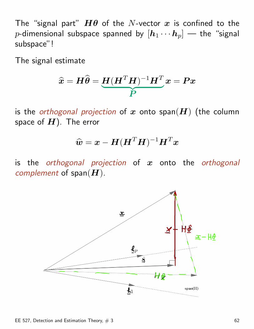
The “signal part” Hθ of the N -vector x is confined to thep-dimensional subspace spanned by [h1 · · ·hp] — the “signalsubspace”!

The signal estimate

x = Hθ = H(HTH)−1HT︸ ︷︷ ︸P

x = Px

is the orthogonal projection of x onto span(H) (the columnspace of H). The error

w = x−H(HTH)−1HTx

is the orthogonal projection of x onto the orthogonalcomplement of span(H).

EE 527, Detection and Estimation Theory, # 3 62

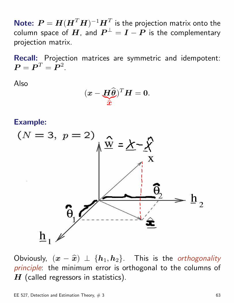
Note: P = H(HTH)−1HT is the projection matrix onto thecolumn space of H, and P⊥ = I − P is the complementaryprojection matrix.

Recall: Projection matrices are symmetric and idempotent:P = P T = P 2.

Also(x− Hθ︸︷︷︸bx )TH = 0.

Example:

Obviously, (x − x) ⊥ {h1,h2}. This is the orthogonalityprinciple: the minimum error is orthogonal to the columns ofH (called regressors in statistics).

EE 527, Detection and Estimation Theory, # 3 63

In general,

x− x ⊥ span(H) ⇔ x− x ⊥ hj, ∀hj ⇔ HT (x−Hθ) = 0.

EE 527, Detection and Estimation Theory, # 3 64

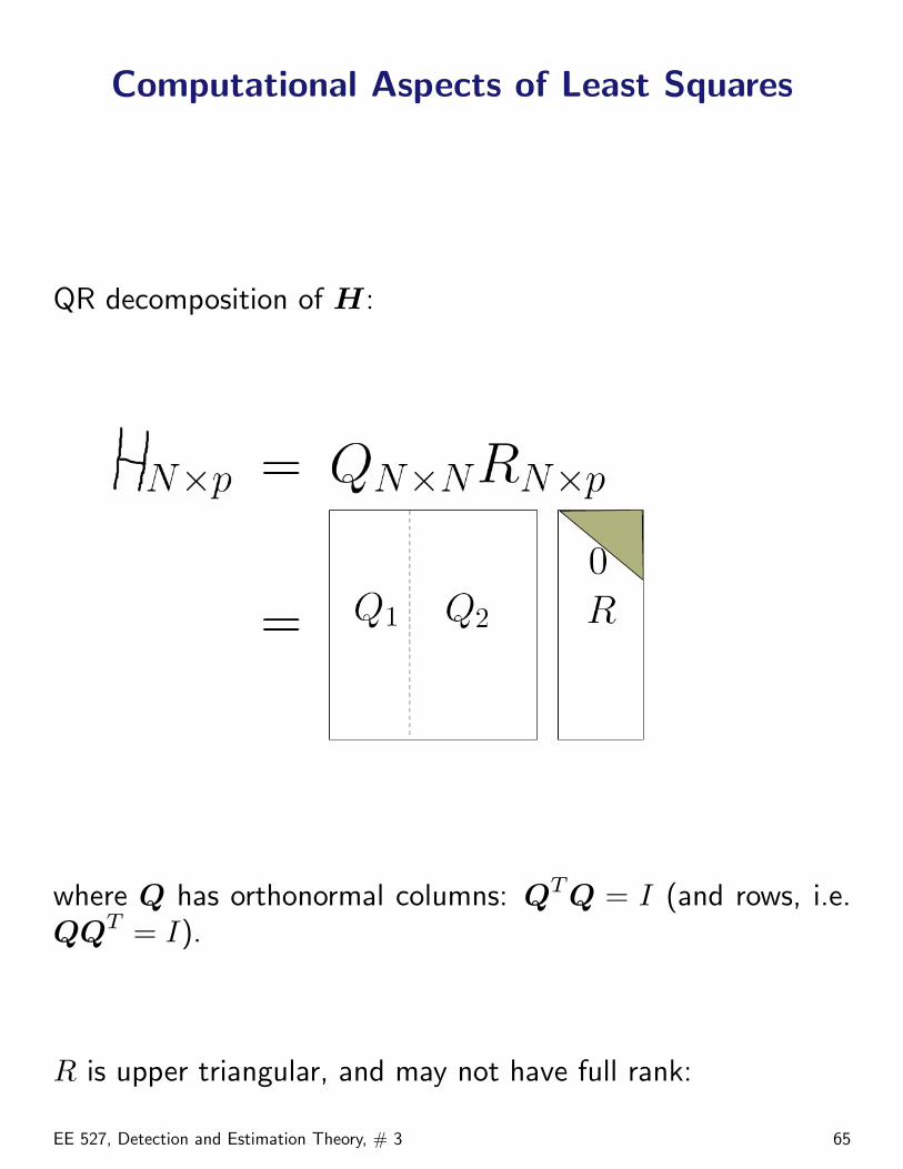
Computational Aspects of Least Squares

QR decomposition of H:

where Q has orthonormal columns: QTQ = I (and rows, i.e.QQT = I).

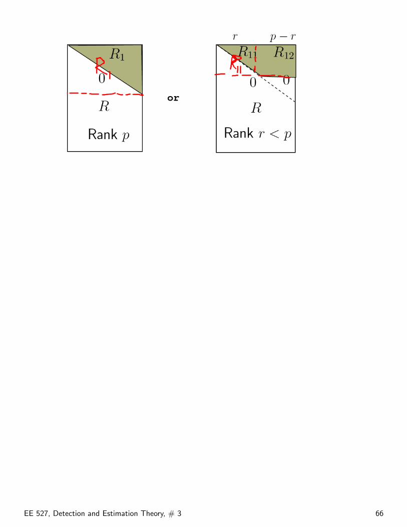
R is upper triangular, and may not have full rank:

EE 527, Detection and Estimation Theory, # 3 65

EE 527, Detection and Estimation Theory, # 3 66

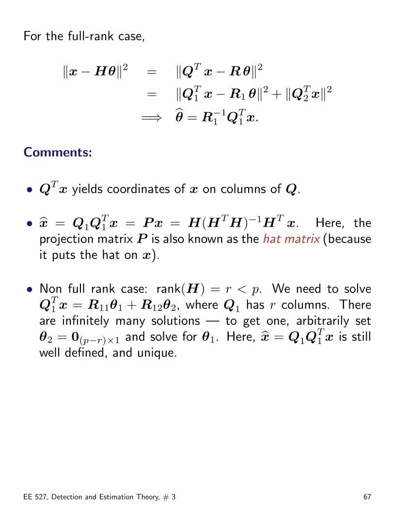
For the full-rank case,

‖x−Hθ‖2 = ‖QT x−R θ‖2

= ‖QT1 x−R1 θ‖2 + ‖QT

2 x‖2

=⇒ θ = R−11 QT

1 x.

Comments:

• QTx yields coordinates of x on columns of Q.

• x = Q1QT1 x = Px = H(HTH)−1HT x. Here, the

projection matrix P is also known as the hat matrix (becauseit puts the hat on x).

• Non full rank case: rank(H) = r < p. We need to solveQT

1 x = R11θ1 + R12θ2, where Q1 has r columns. Thereare infinitely many solutions — to get one, arbitrarily setθ2 = 0(p−r)×1 and solve for θ1. Here, x = Q1Q

T1 x is still

well defined, and unique.

EE 527, Detection and Estimation Theory, # 3 67

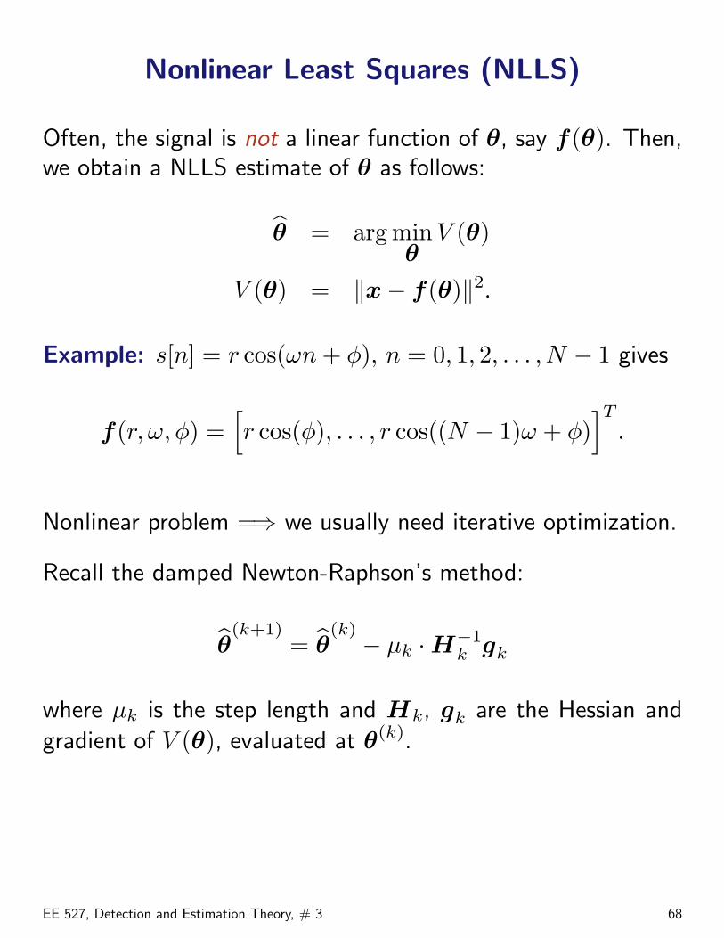
Nonlinear Least Squares (NLLS)

Often, the signal is not a linear function of θ, say f(θ). Then,we obtain a NLLS estimate of θ as follows:

θ = arg minθ

V (θ)

V (θ) = ‖x− f(θ)‖2.

Example: s[n] = r cos(ωn + φ), n = 0, 1, 2, . . . , N − 1 gives

f(r, ω, φ) =[r cos(φ), . . . , r cos((N − 1)ω + φ)

]T

.

Nonlinear problem =⇒ we usually need iterative optimization.

Recall the damped Newton-Raphson’s method:

θ(k+1)

= θ(k)− µk ·H−1

k gk

where µk is the step length and Hk, gk are the Hessian and

gradient of V (θ), evaluated at θ(k).

EE 527, Detection and Estimation Theory, # 3 68

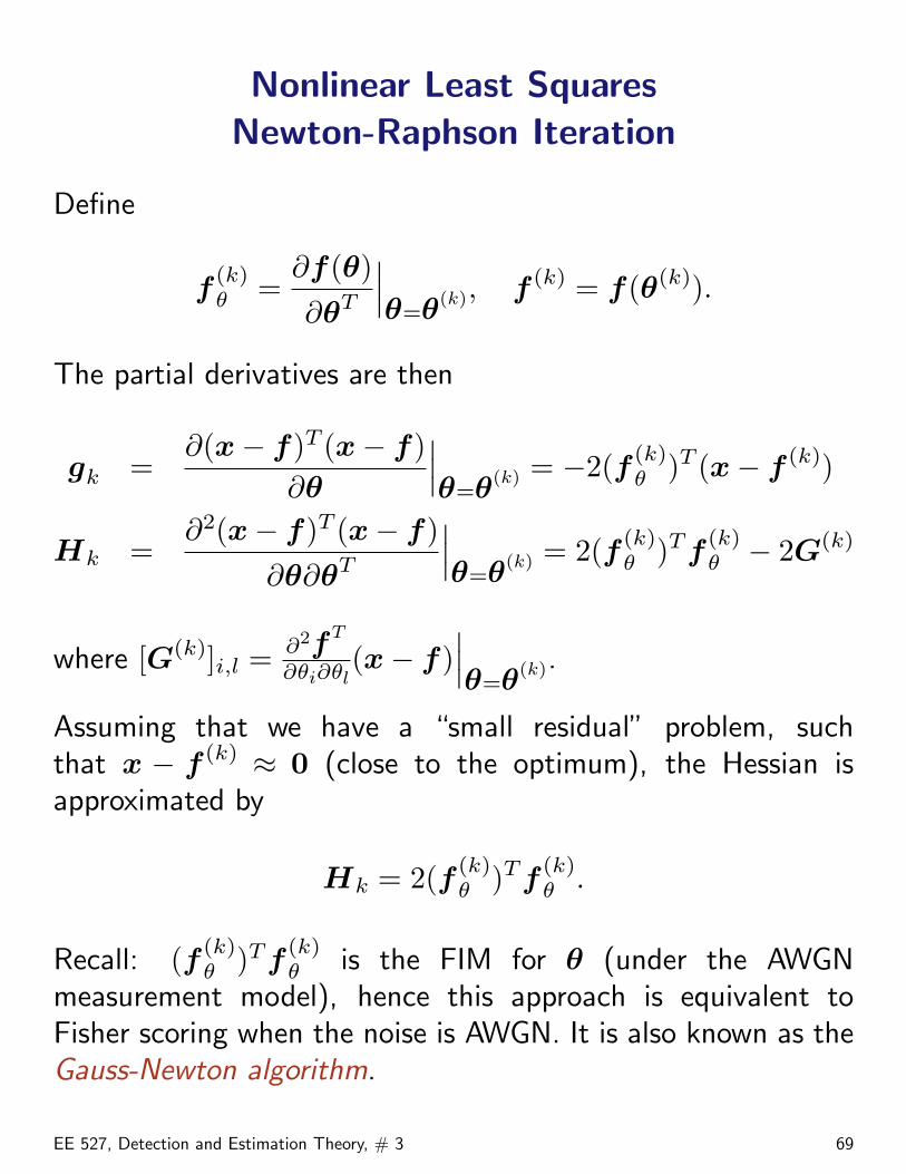
Nonlinear Least SquaresNewton-Raphson Iteration

Define

f(k)θ =

∂f(θ)∂θT

∣∣∣θ=θ(k), f (k) = f(θ(k)).

The partial derivatives are then

gk =∂(x− f)T (x− f)

∂θ

∣∣∣θ=θ(k) = −2(f (k)

θ )T (x− f (k))

Hk =∂2(x− f)T (x− f)

∂θ∂θT

∣∣∣θ=θ(k) = 2(f (k)

θ )Tf(k)θ − 2G(k)

where [G(k)]i,l = ∂2fT

∂θi∂θl(x− f)

∣∣∣θ=θ(k).

Assuming that we have a “small residual” problem, suchthat x − f (k) ≈ 0 (close to the optimum), the Hessian isapproximated by

Hk = 2(f (k)θ )Tf

(k)θ .

Recall: (f (k)θ )Tf

(k)θ is the FIM for θ (under the AWGN

measurement model), hence this approach is equivalent toFisher scoring when the noise is AWGN. It is also known as theGauss-Newton algorithm.

EE 527, Detection and Estimation Theory, # 3 69

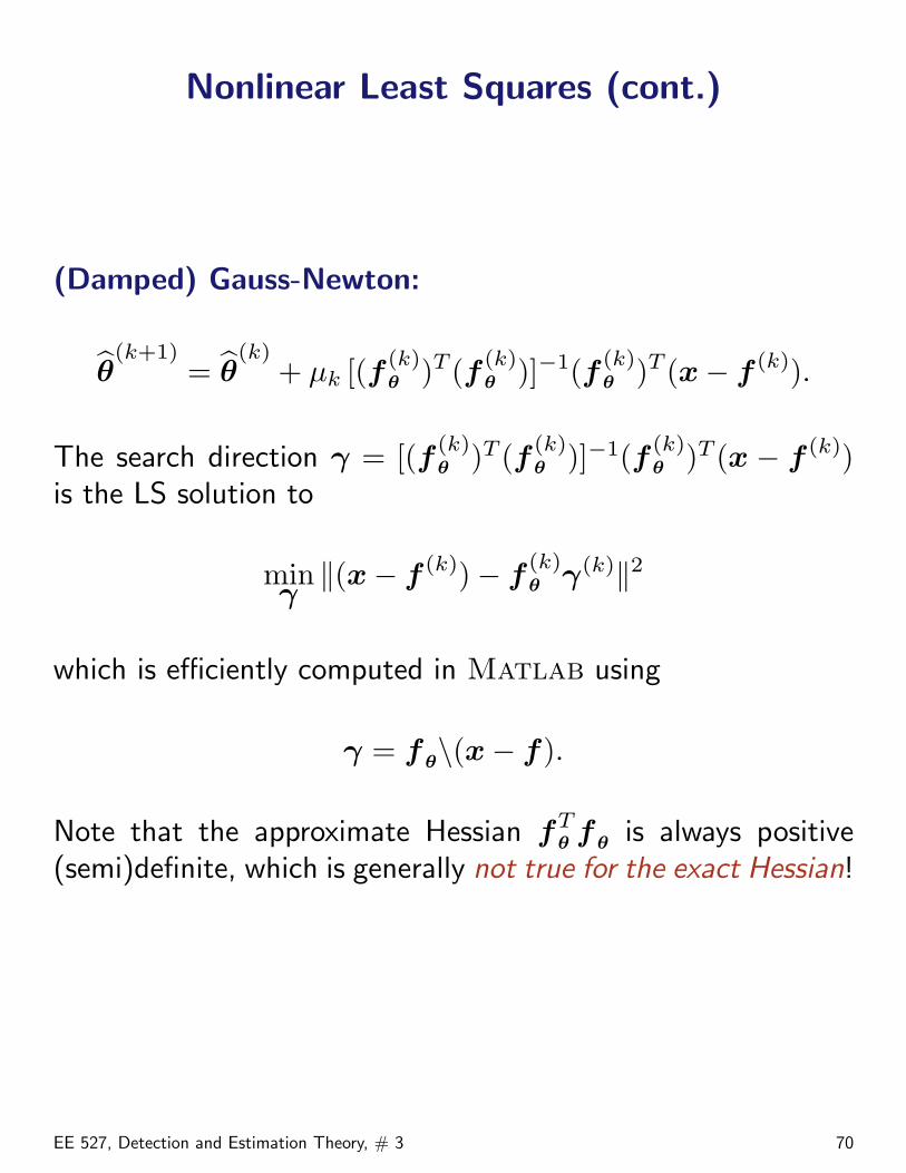
Nonlinear Least Squares (cont.)

(Damped) Gauss-Newton:

θ(k+1)

= θ(k)

+ µk [(f (k)θ )T (f (k)

θ )]−1(f (k)θ )T (x− f (k)).

The search direction γ = [(f (k)θ )T (f (k)

θ )]−1(f (k)θ )T (x − f (k))

is the LS solution to

minγ‖(x− f (k))− f

(k)θ γ(k)‖2

which is efficiently computed in Matlab using

γ = f θ\(x− f).

Note that the approximate Hessian fTθ f θ is always positive

(semi)definite, which is generally not true for the exact Hessian!

EE 527, Detection and Estimation Theory, # 3 70

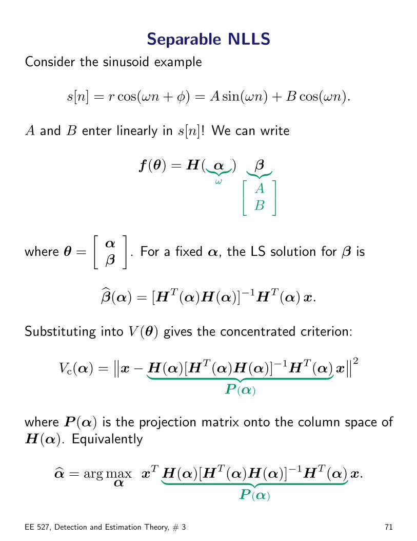
Separable NLLSConsider the sinusoid example

s[n] = r cos(ωn + φ) = A sin(ωn) + B cos(ωn).

A and B enter linearly in s[n]! We can write

f(θ) = H( α︸︷︷︸ω

) β︸︷︷︸24 AB

35

where θ =[

αβ

]. For a fixed α, the LS solution for β is

β(α) = [HT (α)H(α)]−1HT (α) x.

Substituting into V (θ) gives the concentrated criterion:

Vc(α) =∥∥x−H(α)[HT (α)H(α)]−1HT (α)︸ ︷︷ ︸

P (α)

x∥∥2

where P (α) is the projection matrix onto the column space ofH(α). Equivalently

α = arg maxα

xT H(α)[HT (α)H(α)]−1HT (α)︸ ︷︷ ︸P (α)

x.

EE 527, Detection and Estimation Theory, # 3 71

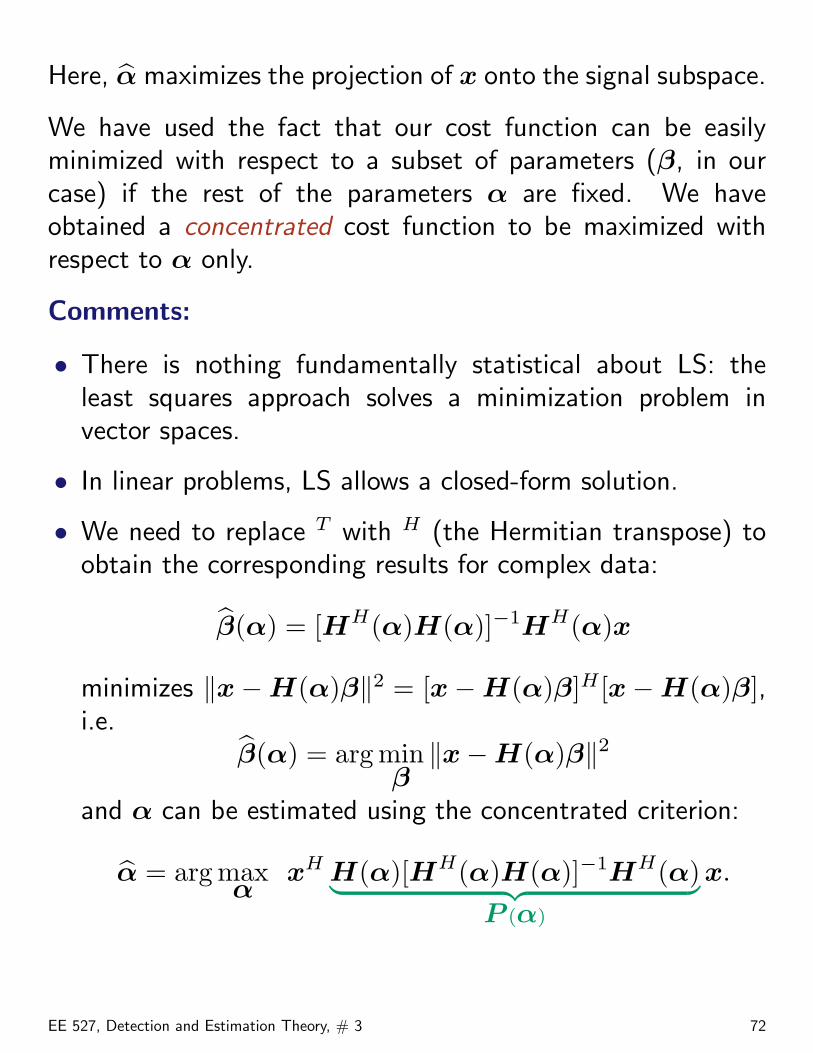
Here, α maximizes the projection of x onto the signal subspace.

We have used the fact that our cost function can be easilyminimized with respect to a subset of parameters (β, in ourcase) if the rest of the parameters α are fixed. We haveobtained a concentrated cost function to be maximized withrespect to α only.

Comments:

• There is nothing fundamentally statistical about LS: theleast squares approach solves a minimization problem invector spaces.

• In linear problems, LS allows a closed-form solution.

• We need to replace T with H (the Hermitian transpose) toobtain the corresponding results for complex data:

β(α) = [HH(α)H(α)]−1HH(α)x

minimizes ‖x−H(α)β‖2 = [x−H(α)β]H[x−H(α)β],i.e.

β(α) = arg minβ‖x−H(α)β‖2

and α can be estimated using the concentrated criterion:

α = arg maxα

xH H(α)[HH(α)H(α)]−1HH(α)︸ ︷︷ ︸P (α)

x.

EE 527, Detection and Estimation Theory, # 3 72