


γλώσσες
Σελίδες
Νομικός


Extending Fisher’s inequality to coverings
Daniel Horsley (Monash University, Australia)

Introduction 1Designs and Fisher’s inequality

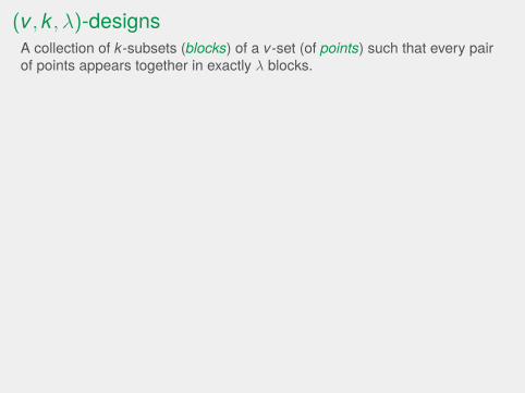
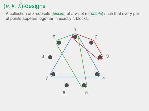
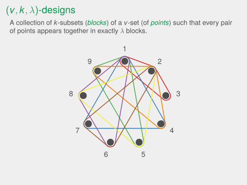
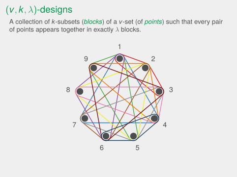
(v, k, λ)-designs
A collection of k-subsets (blocks) of a v-set (of points) such that every pairof points appears together in exactly λ blocks.
12
3
4
56
7
8
9
A (9,3,1)-design with 12 blocks
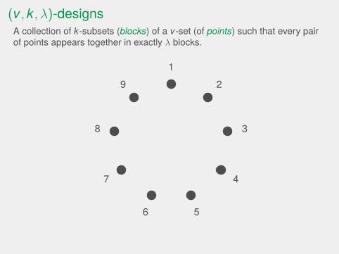
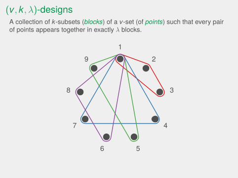
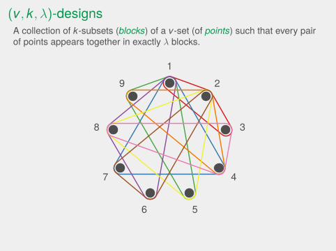
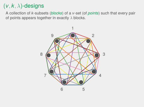
(v, k, λ)-designsA collection of k-subsets (blocks) of a v-set (of points) such that every pairof points appears together in exactly λ blocks.
12
3
4
56
7
8
9
A (9,3,1)-design with 12 blocks
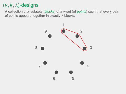
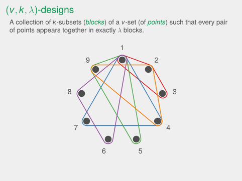
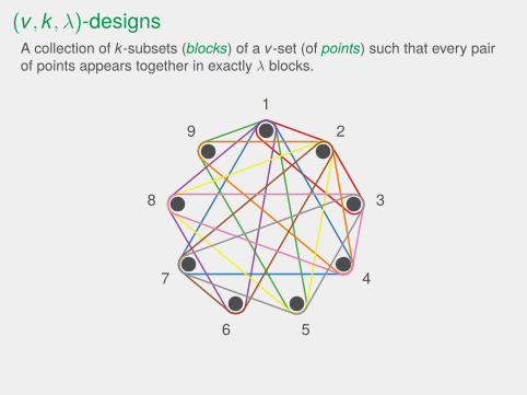
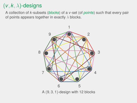
(v, k, λ)-designsA collection of k-subsets (blocks) of a v-set (of points) such that every pairof points appears together in exactly λ blocks.
12
3
4
56
7
8
9
A (9,3,1)-design with 12 blocks
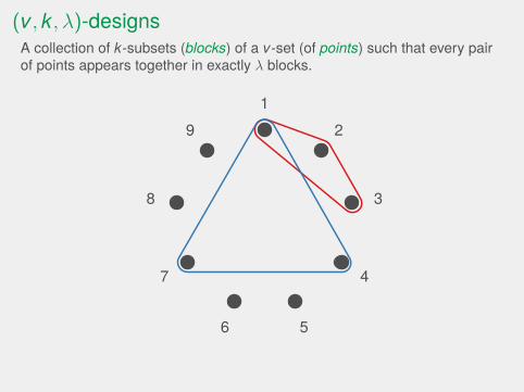
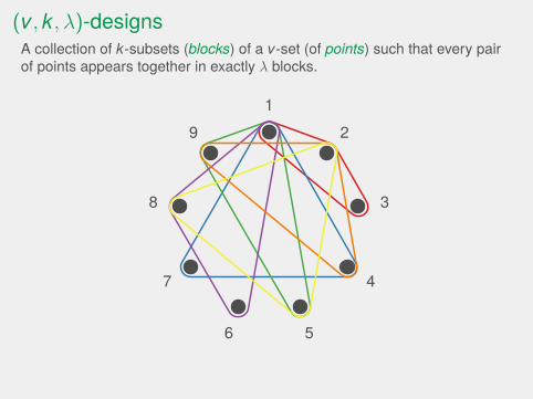
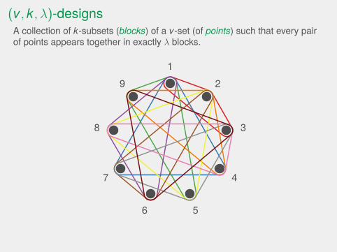
(v, k, λ)-designsA collection of k-subsets (blocks) of a v-set (of points) such that every pairof points appears together in exactly λ blocks.
12
3
4
56
7
8
9
A (9,3,1)-design with 12 blocks
(v, k, λ)-designsA collection of k-subsets (blocks) of a v-set (of points) such that every pairof points appears together in exactly λ blocks.
12
3
4
56
7
8
9
A (9,3,1)-design with 12 blocks
(v, k, λ)-designsA collection of k-subsets (blocks) of a v-set (of points) such that every pairof points appears together in exactly λ blocks.
12
3
4
56
7
8
9
A (9,3,1)-design with 12 blocks
(v, k, λ)-designsA collection of k-subsets (blocks) of a v-set (of points) such that every pairof points appears together in exactly λ blocks.
12
3
4
56
7
8
9
A (9,3,1)-design with 12 blocks
(v, k, λ)-designsA collection of k-subsets (blocks) of a v-set (of points) such that every pairof points appears together in exactly λ blocks.
12
3
4
56
7
8
9
A (9,3,1)-design with 12 blocks
(v, k, λ)-designsA collection of k-subsets (blocks) of a v-set (of points) such that every pairof points appears together in exactly λ blocks.
12
3
4
56
7
8
9
A (9,3,1)-design with 12 blocks
(v, k, λ)-designsA collection of k-subsets (blocks) of a v-set (of points) such that every pairof points appears together in exactly λ blocks.
12
3
4
56
7
8
9
A (9,3,1)-design with 12 blocks
(v, k, λ)-designsA collection of k-subsets (blocks) of a v-set (of points) such that every pairof points appears together in exactly λ blocks.
12
3
4
56
7
8
9
A (9,3,1)-design with 12 blocks
(v, k, λ)-designsA collection of k-subsets (blocks) of a v-set (of points) such that every pairof points appears together in exactly λ blocks.
12
3
4
56
7
8
9
A (9,3,1)-design with 12 blocks
(v, k, λ)-designsA collection of k-subsets (blocks) of a v-set (of points) such that every pairof points appears together in exactly λ blocks.
12
3
4
56
7
8
9
A (9,3,1)-design with 12 blocks
(v, k, λ)-designsA collection of k-subsets (blocks) of a v-set (of points) such that every pairof points appears together in exactly λ blocks.
12
3
4
56
7
8
9
A (9,3,1)-design with 12 blocks
(v, k, λ)-designsA collection of k-subsets (blocks) of a v-set (of points) such that every pairof points appears together in exactly λ blocks.
12
3
4
56
7
8
9
A (9,3,1)-design with 12 blocks
(v, k, λ)-designsA collection of k-subsets (blocks) of a v-set (of points) such that every pairof points appears together in exactly λ blocks.
12
3
4
56
7
8
9
A (9,3,1)-design with 12 blocks

Necessary conditions for a design to exist
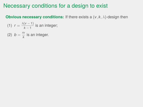
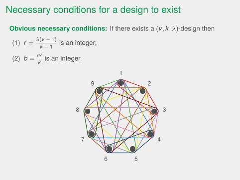
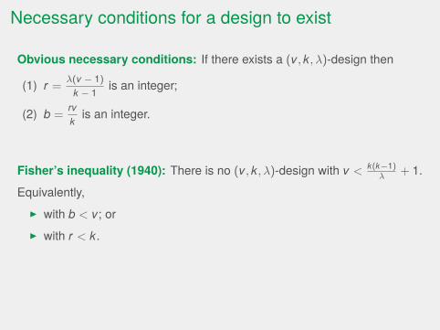
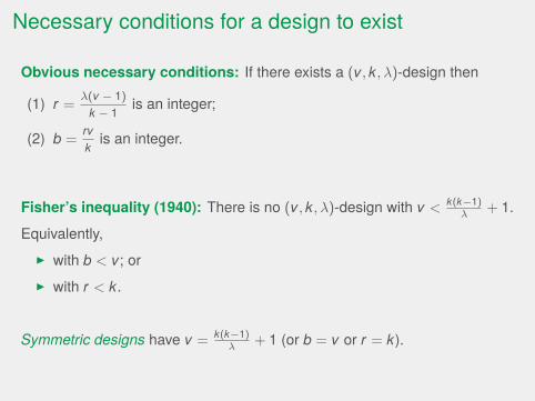
Obvious necessary conditions: If there exists a (v, k, λ)-design then
(1) r = λ(v − 1)k − 1 is an integer;
(2) b =rvk is an integer.
Necessary conditions for a design to exist
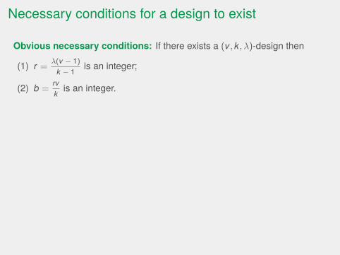
Obvious necessary conditions: If there exists a (v, k, λ)-design then
(1) r = λ(v − 1)k − 1 is an integer;
(2) b =rvk is an integer.
Necessary conditions for a design to exist
Obvious necessary conditions: If there exists a (v, k, λ)-design then
(1) r = λ(v − 1)k − 1 is an integer;
(2) b =rvk is an integer.
12
3
4
56
7
8
9

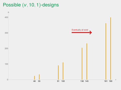
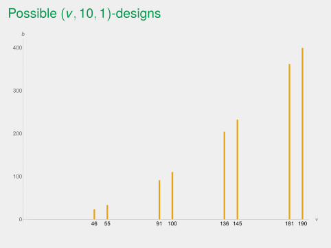
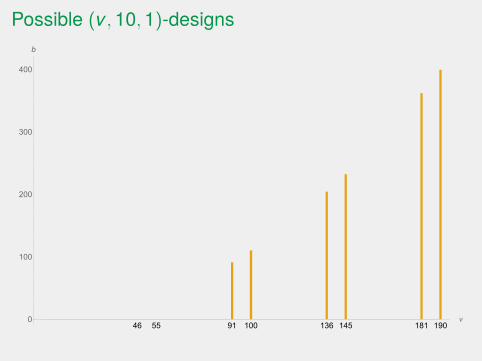
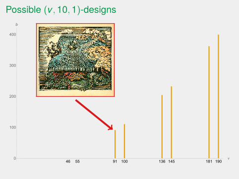
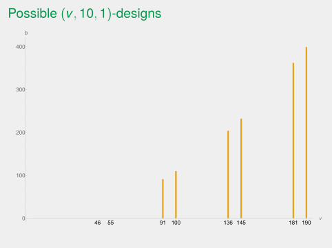
Possible (v,10,1)-designs
46 55 91 100 136 145 181 190v0
100
200
300
400
b
Eventually all exist

Possible (v,10,1)-designs
46 55 91 100 136 145 181 190v0
100
200
300
400
b
Eventually all exist
Possible (v,10,1)-designs
46 55 91 100 136 145 181 190v0
100
200
300
400
b
Eventually all exist
Necessary conditions for a design to exist
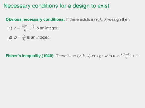
Obvious necessary conditions: If there exists a (v, k, λ)-design then
(1) r = λ(v − 1)k − 1 is an integer;
(2) b =rvk is an integer.
Fisher’s inequality (1940): There is no (v, k, λ)-design with v < k(k−1)λ + 1.
Equivalently,I with b < v; orI with r < k.
Symmetric designs have v = k(k−1)λ + 1 (or b = v or r = k).
Necessary conditions for a design to exist
Obvious necessary conditions: If there exists a (v, k, λ)-design then
(1) r = λ(v − 1)k − 1 is an integer;
(2) b =rvk is an integer.
Fisher’s inequality (1940): There is no (v, k, λ)-design with v < k(k−1)λ + 1.
Equivalently,I with b < v; orI with r < k.
Symmetric designs have v = k(k−1)λ + 1 (or b = v or r = k).

Possible (v,10,1)-designs
46 55 91 100 136 145 181 190v0
100
200
300
400
b
Possible (v,10,1)-designs
46 55 91 100 136 145 181 190v0
100
200
300
400
b
Possible (v,10,1)-designs
46 55 91 100 136 145 181 190v0
100
200
300
400
b
Possible (v,10,1)-designs
46 55 91 100 136 145 181 190v0
100
200
300
400
b
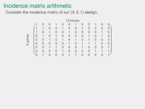
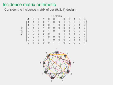
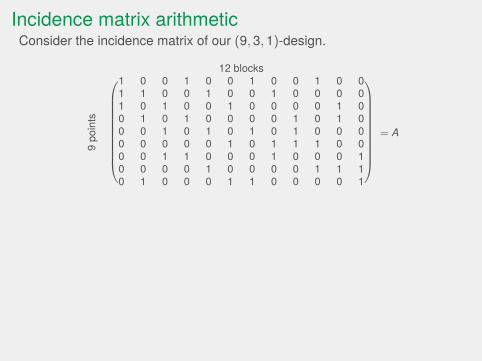
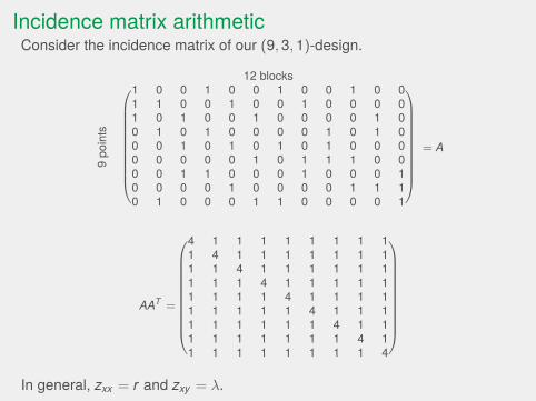
Incidence matrix arithmetic
Consider the incidence matrix of our (9,3,1)-design.
12 blocks
9po
ints
1 0 0 1 0 0 1 0 0 1 0 01 1 0 0 1 0 0 1 0 0 0 01 0 1 0 0 1 0 0 0 0 1 00 1 0 1 0 0 0 0 1 0 1 00 0 1 0 1 0 1 0 1 0 0 00 0 0 0 0 1 0 1 1 1 0 00 0 1 1 0 0 0 1 0 0 0 10 0 0 0 1 0 0 0 0 1 1 10 1 0 0 0 1 1 0 0 0 0 1
Incidence matrix arithmeticConsider the incidence matrix of our (9,3,1)-design.
12 blocks
9po
ints
1 0 0 1 0 0 1 0 0 1 0 01 1 0 0 1 0 0 1 0 0 0 01 0 1 0 0 1 0 0 0 0 1 00 1 0 1 0 0 0 0 1 0 1 00 0 1 0 1 0 1 0 1 0 0 00 0 0 0 0 1 0 1 1 1 0 00 0 1 1 0 0 0 1 0 0 0 10 0 0 0 1 0 0 0 0 1 1 10 1 0 0 0 1 1 0 0 0 0 1
12
3
4
56
7
8
9

Incidence matrix arithmeticConsider the incidence matrix of our (9,3,1)-design.
12 blocks
9po
ints
1 0 0 1 0 0 1 0 0 1 0 01 1 0 0 1 0 0 1 0 0 0 01 0 1 0 0 1 0 0 0 0 1 00 1 0 1 0 0 0 0 1 0 1 00 0 1 0 1 0 1 0 1 0 0 00 0 0 0 0 1 0 1 1 1 0 00 0 1 1 0 0 0 1 0 0 0 10 0 0 0 1 0 0 0 0 1 1 10 1 0 0 0 1 1 0 0 0 0 1
Incidence matrix arithmeticConsider the incidence matrix of our (9,3,1)-design.
12 blocks
9po
ints
= A
1 0 0 1 0 0 1 0 0 1 0 01 1 0 0 1 0 0 1 0 0 0 01 0 1 0 0 1 0 0 0 0 1 00 1 0 1 0 0 0 0 1 0 1 00 0 1 0 1 0 1 0 1 0 0 00 0 0 0 0 1 0 1 1 1 0 00 0 1 1 0 0 0 1 0 0 0 10 0 0 0 1 0 0 0 0 1 1 10 1 0 0 0 1 1 0 0 0 0 1
AAT =
4 1 1 1 1 1 1 1 11 4 1 1 1 1 1 1 11 1 4 1 1 1 1 1 11 1 1 4 1 1 1 1 11 1 1 1 4 1 1 1 11 1 1 1 1 4 1 1 11 1 1 1 1 1 4 1 11 1 1 1 1 1 1 4 11 1 1 1 1 1 1 1 4
In general, zxx = r and zxy = λ.

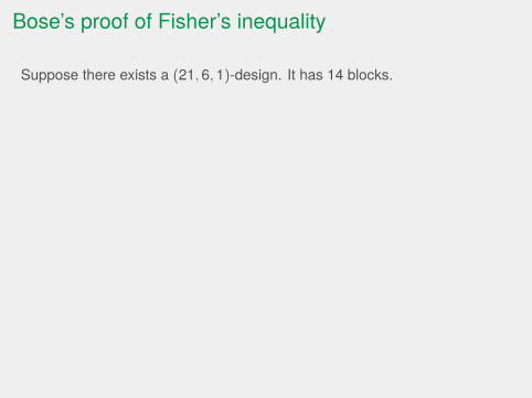
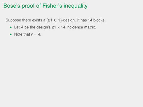
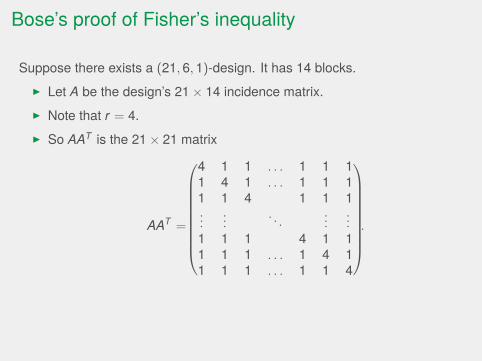
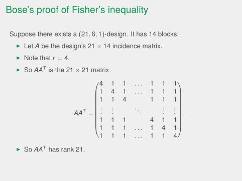
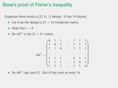
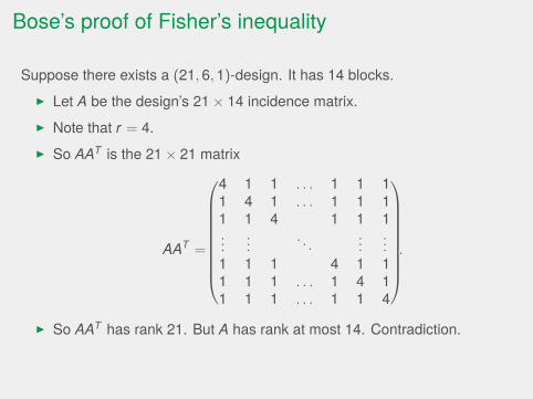
Bose’s proof of Fisher’s inequality
Suppose there exists a (21,6,1)-design. It has 14 blocks.I Let A be the design’s 21 × 14 incidence matrix.I Note that r = 4.I So AAT is the 21 × 21 matrix
AAT =
4 1 1 . . . 1 1 11 4 1 . . . 1 1 11 1 4 1 1 1...
.... . .
......
1 1 1 4 1 11 1 1 . . . 1 4 11 1 1 . . . 1 1 4
.
I So AAT has rank 21. But A has rank at most 14. Contradiction.

Bose’s proof of Fisher’s inequality
Suppose there exists a (21,6,1)-design.
It has 14 blocks.I Let A be the design’s 21 × 14 incidence matrix.I Note that r = 4.I So AAT is the 21 × 21 matrix
AAT =
4 1 1 . . . 1 1 11 4 1 . . . 1 1 11 1 4 1 1 1...
.... . .
......
1 1 1 4 1 11 1 1 . . . 1 4 11 1 1 . . . 1 1 4
.
I So AAT has rank 21. But A has rank at most 14. Contradiction.
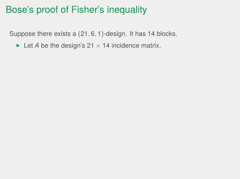
Bose’s proof of Fisher’s inequality
Suppose there exists a (21,6,1)-design. It has 14 blocks.
I Let A be the design’s 21 × 14 incidence matrix.I Note that r = 4.I So AAT is the 21 × 21 matrix
AAT =
4 1 1 . . . 1 1 11 4 1 . . . 1 1 11 1 4 1 1 1...
.... . .
......
1 1 1 4 1 11 1 1 . . . 1 4 11 1 1 . . . 1 1 4
.
I So AAT has rank 21. But A has rank at most 14. Contradiction.
Bose’s proof of Fisher’s inequality
Suppose there exists a (21,6,1)-design. It has 14 blocks.I Let A be the design’s 21 × 14 incidence matrix.
I Note that r = 4.I So AAT is the 21 × 21 matrix
AAT =
4 1 1 . . . 1 1 11 4 1 . . . 1 1 11 1 4 1 1 1...
.... . .
......
1 1 1 4 1 11 1 1 . . . 1 4 11 1 1 . . . 1 1 4
.
I So AAT has rank 21. But A has rank at most 14. Contradiction.
Bose’s proof of Fisher’s inequality
Suppose there exists a (21,6,1)-design. It has 14 blocks.I Let A be the design’s 21 × 14 incidence matrix.I Note that r = 4.
I So AAT is the 21 × 21 matrix
AAT =
4 1 1 . . . 1 1 11 4 1 . . . 1 1 11 1 4 1 1 1...
.... . .
......
1 1 1 4 1 11 1 1 . . . 1 4 11 1 1 . . . 1 1 4
.
I So AAT has rank 21. But A has rank at most 14. Contradiction.
Bose’s proof of Fisher’s inequality
Suppose there exists a (21,6,1)-design. It has 14 blocks.I Let A be the design’s 21 × 14 incidence matrix.I Note that r = 4.I So AAT is the 21 × 21 matrix
AAT =
4 1 1 . . . 1 1 11 4 1 . . . 1 1 11 1 4 1 1 1...
.... . .
......
1 1 1 4 1 11 1 1 . . . 1 4 11 1 1 . . . 1 1 4
.
I So AAT has rank 21. But A has rank at most 14. Contradiction.
Bose’s proof of Fisher’s inequality
Suppose there exists a (21,6,1)-design. It has 14 blocks.I Let A be the design’s 21 × 14 incidence matrix.I Note that r = 4.I So AAT is the 21 × 21 matrix
AAT =
4 1 1 . . . 1 1 11 4 1 . . . 1 1 11 1 4 1 1 1...
.... . .
......
1 1 1 4 1 11 1 1 . . . 1 4 11 1 1 . . . 1 1 4
.
I So AAT has rank 21.
But A has rank at most 14. Contradiction.
Bose’s proof of Fisher’s inequality
Suppose there exists a (21,6,1)-design. It has 14 blocks.I Let A be the design’s 21 × 14 incidence matrix.I Note that r = 4.I So AAT is the 21 × 21 matrix
AAT =
4 1 1 . . . 1 1 11 4 1 . . . 1 1 11 1 4 1 1 1...
.... . .
......
1 1 1 4 1 11 1 1 . . . 1 4 11 1 1 . . . 1 1 4
.
I So AAT has rank 21. But A has rank at most 14.
Contradiction.
Bose’s proof of Fisher’s inequality
Suppose there exists a (21,6,1)-design. It has 14 blocks.I Let A be the design’s 21 × 14 incidence matrix.I Note that r = 4.I So AAT is the 21 × 21 matrix
AAT =
4 1 1 . . . 1 1 11 4 1 . . . 1 1 11 1 4 1 1 1...
.... . .
......
1 1 1 4 1 11 1 1 . . . 1 4 11 1 1 . . . 1 1 4
.
I So AAT has rank 21. But A has rank at most 14. Contradiction.

Introduction 2Coverings and the Schonheim bound

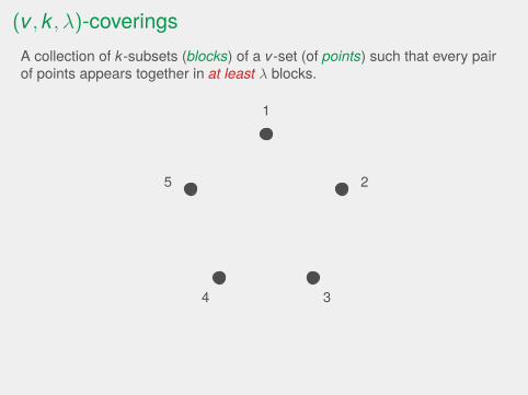
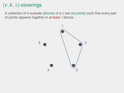
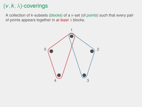
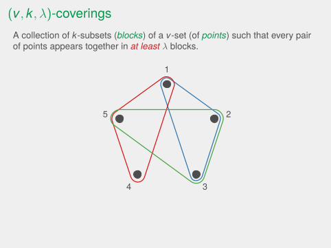
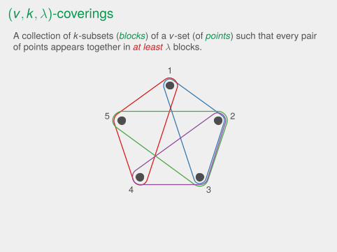
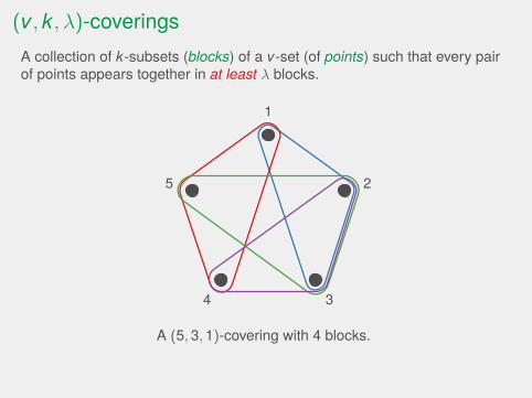
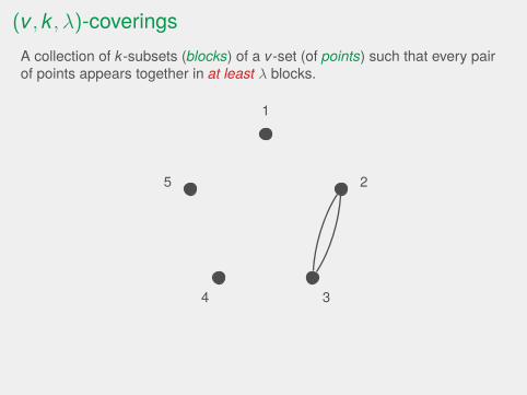
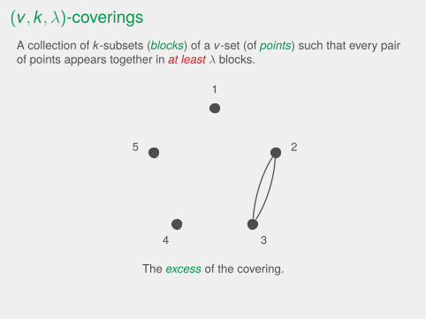
(v, k, λ)-coverings
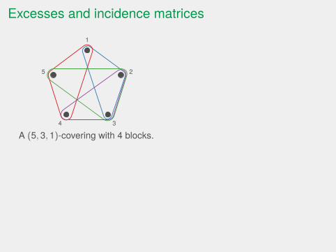
A collection of k-subsets (blocks) of a v-set (of points) such that every pairof points appears together in at least λ blocks.
1
2
34
5
(v, k, λ)-coveringsA collection of k-subsets (blocks) of a v-set (of points) such that every pairof points appears together in at least λ blocks.
1
2
34
5
(v, k, λ)-coveringsA collection of k-subsets (blocks) of a v-set (of points) such that every pairof points appears together in at least λ blocks.
1
2
34
5
(v, k, λ)-coveringsA collection of k-subsets (blocks) of a v-set (of points) such that every pairof points appears together in at least λ blocks.
1
2
34
5
(v, k, λ)-coveringsA collection of k-subsets (blocks) of a v-set (of points) such that every pairof points appears together in at least λ blocks.
1
2
34
5
(v, k, λ)-coveringsA collection of k-subsets (blocks) of a v-set (of points) such that every pairof points appears together in at least λ blocks.
1
2
34
5
(v, k, λ)-coveringsA collection of k-subsets (blocks) of a v-set (of points) such that every pairof points appears together in at least λ blocks.
1
2
34
5
(v, k, λ)-coveringsA collection of k-subsets (blocks) of a v-set (of points) such that every pairof points appears together in at least λ blocks.
1
2
34
5
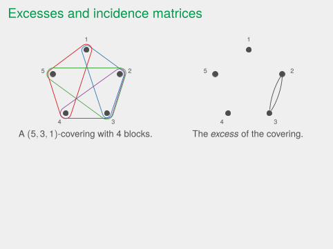
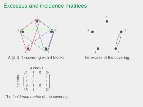
A (5,3,1)-covering with 4 blocks.
(v, k, λ)-coveringsA collection of k-subsets (blocks) of a v-set (of points) such that every pairof points appears together in at least λ blocks.
1
2
34
5
(v, k, λ)-coveringsA collection of k-subsets (blocks) of a v-set (of points) such that every pairof points appears together in at least λ blocks.
1
2
34
5
The excess of the covering.

Coverings
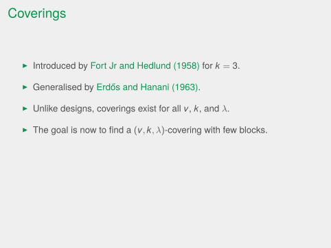
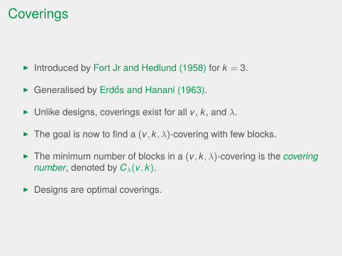
I Introduced by Fort Jr and Hedlund (1958) for k = 3.
I Generalised by Erdos and Hanani (1963).
I Unlike designs, coverings exist for all v, k, and λ.
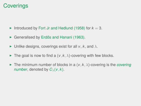
I The goal is now to find a (v, k, λ)-covering with few blocks.
I The minimum number of blocks in a (v, k, λ)-covering is the coveringnumber, denoted by Cλ(v, k).
I Designs are optimal coverings.

Coverings
I Introduced by Fort Jr and Hedlund (1958) for k = 3.
I Generalised by Erdos and Hanani (1963).
I Unlike designs, coverings exist for all v, k, and λ.
I The goal is now to find a (v, k, λ)-covering with few blocks.
I The minimum number of blocks in a (v, k, λ)-covering is the coveringnumber, denoted by Cλ(v, k).
I Designs are optimal coverings.

The Schonheim bound
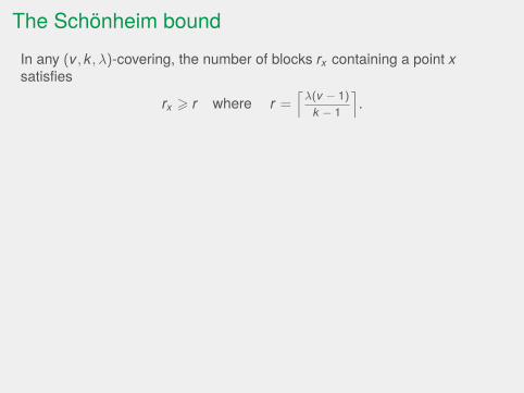
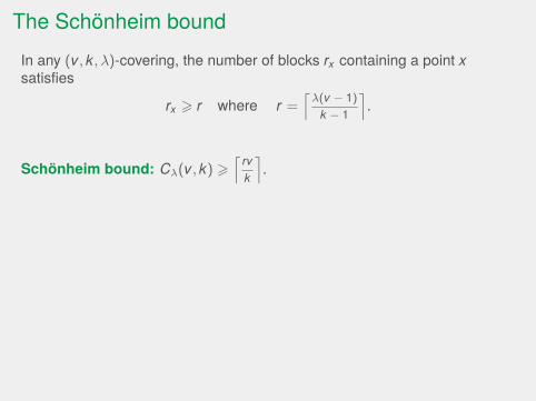
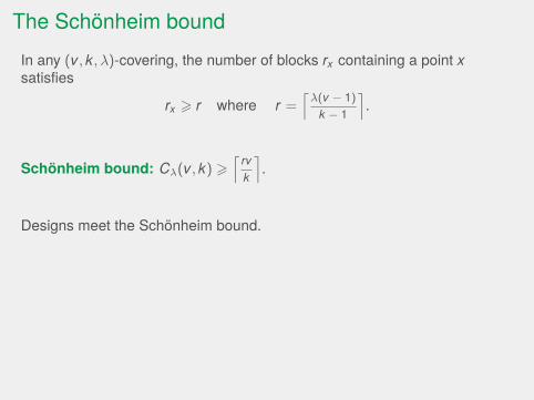
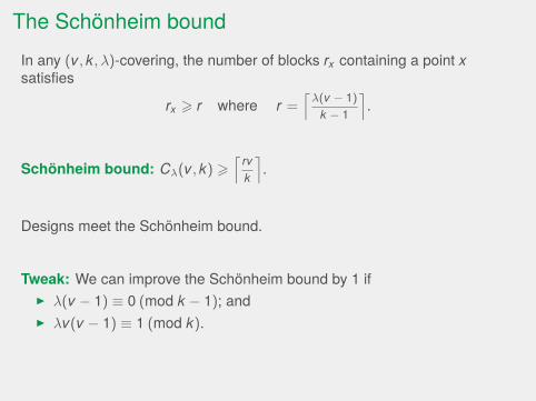
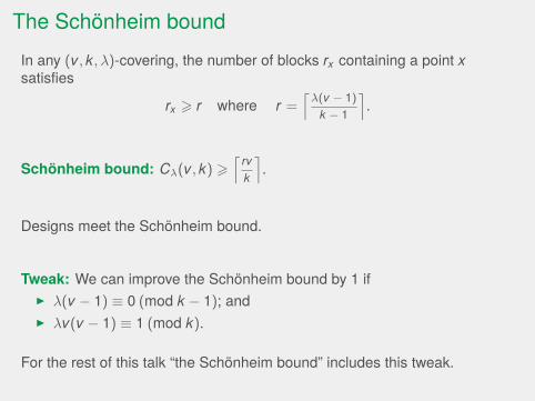
In any (v, k, λ)-covering, the number of blocks rx containing a point xsatisfies
rx > r where r =⌈λ(v − 1)
k − 1
⌉.
Schonheim bound: Cλ(v, k) >⌈ rv
k
⌉.
Designs meet the Schonheim bound.
Tweak: We can improve the Schonheim bound by 1 ifI λ(v − 1) ≡ 0 (mod k − 1); andI λv(v − 1) ≡ 1 (mod k).
For the rest of this talk “the Schonheim bound” includes this tweak.
The Schonheim boundIn any (v, k, λ)-covering, the number of blocks rx containing a point xsatisfies
rx > r where r =⌈λ(v − 1)
k − 1
⌉.
Schonheim bound: Cλ(v, k) >⌈ rv
k
⌉.
Designs meet the Schonheim bound.
Tweak: We can improve the Schonheim bound by 1 ifI λ(v − 1) ≡ 0 (mod k − 1); andI λv(v − 1) ≡ 1 (mod k).
For the rest of this talk “the Schonheim bound” includes this tweak.

Possible (v,10,1)-designs
46 55 91 100 136 145 181 190v0
100
200
300
400
b
Eventually all exist
subsymmetric coverings
Possible (v,10,1)-designs
46 55 91 100 136 145 181 190v0
100
200
300
400
b
Eventually all exist
subsymmetric coverings

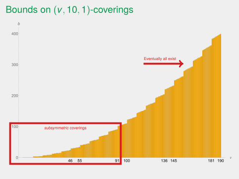
Bounds on (v,10,1)-coverings
46 55 91 100 136 145 181 190v0
100
200
300
400
b
Eventually all exist
subsymmetric coverings

Bounds on (v,10,1)-coverings
46 55 91 100 136 145 181 190v0
100
200
300
400
b
Eventually all exist
subsymmetric coverings
Bounds on (v,10,1)-coverings
46 55 91 100 136 145 181 190v0
100
200
300
400
b
Eventually all exist
subsymmetric coverings
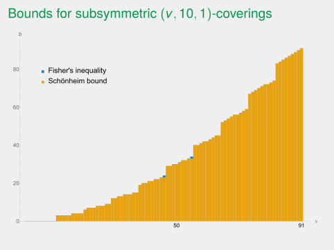
Possible subsymmetric (v,10,1)-coverings
50 91v
Fisher's inequality
Schönheim bound
0
20
40
60
80
b

Possible subsymmetric (v,10,1)-coverings
50 91v
Fisher's inequality
Schönheim bound
0
20
40
60
80
b

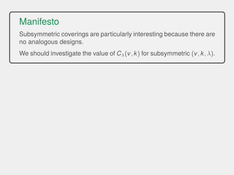
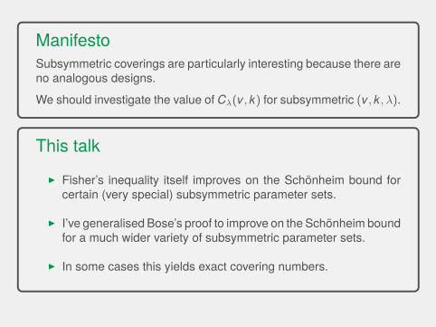
ManifestoSubsymmetric coverings are particularly interesting because there areno analogous designs.
We should investigate the value of Cλ(v, k) for subsymmetric (v, k, λ).
This talkI Fisher’s inequality itself improves on the Schonheim bound for
certain (very special) subsymmetric parameter sets.
I I’ve generalised Bose’s proof to improve on the Schonheim boundfor a much wider variety of subsymmetric parameter sets.
I In some cases this yields exact covering numbers.

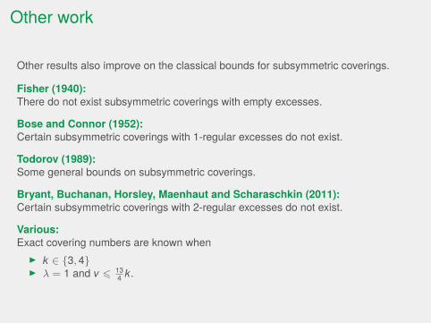
Other work
Other results also improve on the classical bounds for subsymmetric coverings.
Fisher (1940):There do not exist subsymmetric coverings with empty excesses.
Bose and Connor (1952):Certain subsymmetric coverings with 1-regular excesses do not exist.
Todorov (1989):Some general bounds on subsymmetric coverings.
Bryant, Buchanan, Horsley, Maenhaut and Scharaschkin (2011):Certain subsymmetric coverings with 2-regular excesses do not exist.
Various:Exact covering numbers are known when
I k ∈ {3, 4}I λ = 1 and v 6 13
4 k.

Part 1A simple new bound

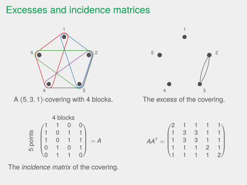
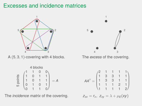
Excesses and incidence matrices
1
2
34
5
A (5,3,1)-covering with 4 blocks.
1
2
34
5
The excess of the covering.
4 blocks
5po
ints
1 1 0 01 0 1 11 0 1 10 1 0 10 1 1 0
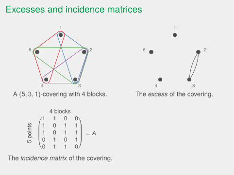
The incidence matrix of the covering.
AAT =
2 1 1 1 11 3 3 1 11 3 3 1 11 1 1 2 11 1 1 1 2
zxx = rx , zxy = λ+ µE(xy)
Excesses and incidence matrices
1
2
34
5
A (5,3,1)-covering with 4 blocks.
1
2
34
5
The excess of the covering.
4 blocks
5po
ints
1 1 0 01 0 1 11 0 1 10 1 0 10 1 1 0
The incidence matrix of the covering.
AAT =
2 1 1 1 11 3 3 1 11 3 3 1 11 1 1 2 11 1 1 1 2
zxx = rx , zxy = λ+ µE(xy)
Excesses and incidence matrices
1
2
34
5
A (5,3,1)-covering with 4 blocks.
1
2
34
5
The excess of the covering.
4 blocks
5po
ints
1 1 0 01 0 1 11 0 1 10 1 0 10 1 1 0
The incidence matrix of the covering.
AAT =
2 1 1 1 11 3 3 1 11 3 3 1 11 1 1 2 11 1 1 1 2
zxx = rx , zxy = λ+ µE(xy)
Excesses and incidence matrices
1
2
34
5
A (5,3,1)-covering with 4 blocks.
1
2
34
5
The excess of the covering.
4 blocks
5po
ints
1 1 0 01 0 1 11 0 1 10 1 0 10 1 1 0
The incidence matrix of the covering.
AAT =
2 1 1 1 11 3 3 1 11 3 3 1 11 1 1 2 11 1 1 1 2
zxx = rx , zxy = λ+ µE(xy)
Excesses and incidence matrices
1
2
34
5
A (5,3,1)-covering with 4 blocks.
1
2
34
5
The excess of the covering.
4 blocks
5po
ints
= A
1 1 0 01 0 1 11 0 1 10 1 0 10 1 1 0
The incidence matrix of the covering.
AAT =
2 1 1 1 11 3 3 1 11 3 3 1 11 1 1 2 11 1 1 1 2
zxx = rx , zxy = λ+ µE(xy)
Excesses and incidence matrices
1
2
34
5
A (5,3,1)-covering with 4 blocks.
1
2
34
5
The excess of the covering.
4 blocks
5po
ints
= A
1 1 0 01 0 1 11 0 1 10 1 0 10 1 1 0
The incidence matrix of the covering.
AAT =
2 1 1 1 11 3 3 1 11 3 3 1 11 1 1 2 11 1 1 1 2
zxx = rx , zxy = λ+ µE(xy)
Excesses and incidence matrices
1
2
34
5
A (5,3,1)-covering with 4 blocks.
1
2
34
5
The excess of the covering.
4 blocks
5po
ints
= A
1 1 0 01 0 1 11 0 1 10 1 0 10 1 1 0
The incidence matrix of the covering.
AAT =
2 1 1 1 11 3 3 1 11 3 3 1 11 1 1 2 11 1 1 1 2
zxx = rx , zxy = λ+ µE(xy)

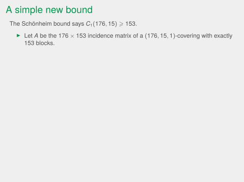
A simple new bound
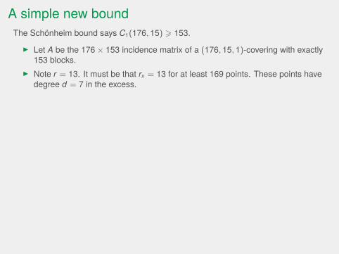
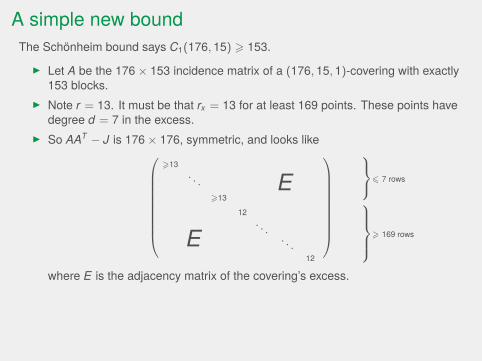
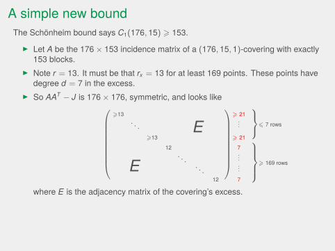
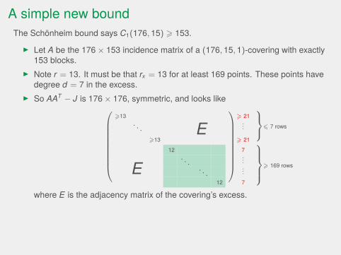
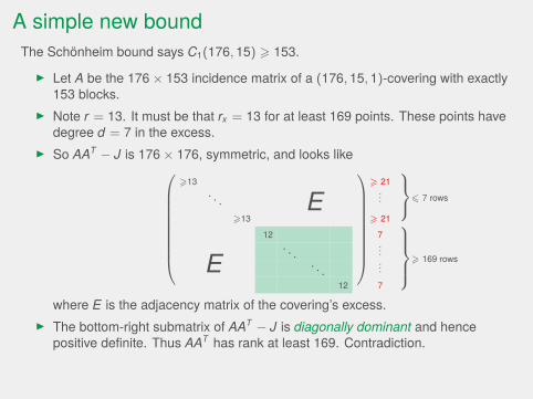
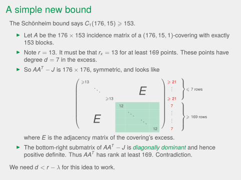
The Schonheim bound says C1(176, 15) > 153.
I Let A be the 176× 153 incidence matrix of a (176, 15, 1)-covering with exactly153 blocks.
I Note r = 13. It must be that rx = 13 for at least 169 points. These points havedegree d = 7 in the excess.
I So AAT − J is 176× 176, symmetric, and looks like
>13
> 21
6 7 rows. . . E
...
>13
> 21
12
7
> 169 rows. . .
...
E . . .
...
12
7
where E is the adjacency matrix of the covering’s excess.I The bottom-right submatrix of AAT − J is diagonally dominant and hence
positive definite. Thus AAT has rank at least 169. Contradiction.
We need d < r − λ for this idea to work.
A simple new boundThe Schonheim bound says C1(176, 15) > 153.
I Let A be the 176× 153 incidence matrix of a (176, 15, 1)-covering with exactly153 blocks.
I Note r = 13. It must be that rx = 13 for at least 169 points. These points havedegree d = 7 in the excess.
I So AAT − J is 176× 176, symmetric, and looks like
>13
> 21
6 7 rows. . . E
...
>13
> 21
12
7
> 169 rows. . .
...
E . . .
...
12
7
where E is the adjacency matrix of the covering’s excess.
I The bottom-right submatrix of AAT − J is diagonally dominant and hencepositive definite. Thus AAT has rank at least 169. Contradiction.
We need d < r − λ for this idea to work.
A simple new boundThe Schonheim bound says C1(176, 15) > 153.
I Let A be the 176× 153 incidence matrix of a (176, 15, 1)-covering with exactly153 blocks.
I Note r = 13. It must be that rx = 13 for at least 169 points. These points havedegree d = 7 in the excess.
I So AAT − J is 176× 176, symmetric, and looks like
>13
> 216 7 rows. . . E ...
>13 > 21
12 7> 169 rows
. . ....E . . ....
12 7
where E is the adjacency matrix of the covering’s excess.I The bottom-right submatrix of AAT − J is diagonally dominant and hence
positive definite. Thus AAT has rank at least 169. Contradiction.
We need d < r − λ for this idea to work.
A simple new boundThe Schonheim bound says C1(176, 15) > 153.
I Let A be the 176× 153 incidence matrix of a (176, 15, 1)-covering with exactly153 blocks.
I Note r = 13. It must be that rx = 13 for at least 169 points. These points havedegree d = 7 in the excess.
I So AAT − J is 176× 176, symmetric, and looks like
>13
> 216 7 rows. . . E ...
>13 > 21
12 7> 169 rows
. . ....E . . ....
12 7
where E is the adjacency matrix of the covering’s excess.I The bottom-right submatrix of AAT − J is diagonally dominant and hence
positive definite. Thus AAT has rank at least 169. Contradiction.
We need d < r − λ for this idea to work.

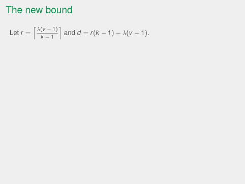
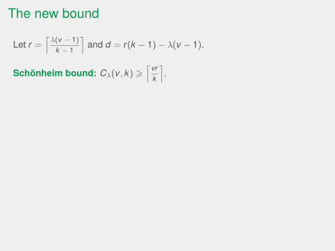
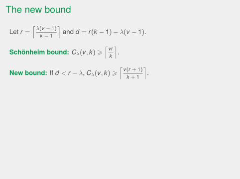
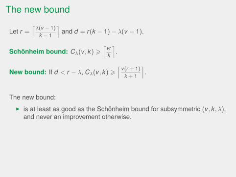
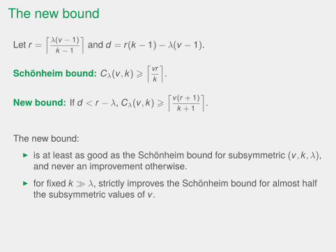
The new bound
Let r =⌈λ(v − 1)
k − 1
⌉and d = r(k − 1)− λ(v − 1).
Schonheim bound: Cλ(v, k) >⌈vr
k
⌉.
New bound: If d < r − λ, Cλ(v, k) >⌈v(r + 1)
k + 1
⌉.
The new bound:I is at least as good as the Schonheim bound for subsymmetric (v, k, λ),
and never an improvement otherwise.I for fixed k � λ, strictly improves the Schonheim bound for almost half
the subsymmetric values of v.I generalises Fisher’s inequality.
The new bound
Let r =⌈λ(v − 1)
k − 1
⌉and d = r(k − 1)− λ(v − 1).
Schonheim bound: Cλ(v, k) >⌈ vr
k
⌉.
New bound: If d < r − λ, Cλ(v, k) >⌈v(r + 1)
k + 1
⌉.
The new bound:I is at least as good as the Schonheim bound for subsymmetric (v, k, λ),
and never an improvement otherwise.
I for fixed k � λ, strictly improves the Schonheim bound for almost halfthe subsymmetric values of v.
I generalises Fisher’s inequality.
The new bound
Let r =⌈λ(v − 1)
k − 1
⌉and d = r(k − 1)− λ(v − 1).
Schonheim bound: Cλ(v, k) >⌈ vr
k
⌉.
New bound: If d < r − λ, Cλ(v, k) >⌈v(r + 1)
k + 1
⌉.
The new bound:I is at least as good as the Schonheim bound for subsymmetric (v, k, λ),
and never an improvement otherwise.I for fixed k � λ, strictly improves the Schonheim bound for almost half
the subsymmetric values of v.
I generalises Fisher’s inequality.

The new bound
Let r =⌈λ(v − 1)
k − 1
⌉and d = r(k − 1)− λ(v − 1).
Schonheim bound: Cλ(v, k) >⌈ vr
k
⌉.
New bound: If d < r − λ, Cλ(v, k) >⌈v(r + 1)
k + 1
⌉.
The new bound:I is at least as good as the Schonheim bound for subsymmetric (v, k, λ),
and never an improvement otherwise.I for fixed k � λ, strictly improves the Schonheim bound for almost half
the subsymmetric values of v.I generalises Fisher’s inequality.

Bounds for subsymmetric (v,10,1)-coverings
50 91v
Fisher's inequality
Schönheim bound
0
20
40
60
80
b
Bounds for subsymmetric (v,10,1)-coverings
50 91v
Fisher's inequality
Schönheim bound
0
20
40
60
80
b
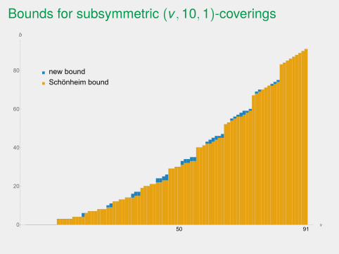
Bounds for subsymmetric (v,10,1)-coverings
50 91v
new bound
Schönheim bound
0
20
40
60
80
b
Bounds for subsymmetric (v,15,1)-coverings
50 100 150 200 211v
new bound
Schönheim bound
0
50
100
150
200
b
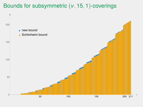
Bounds for subsymmetric (v,15,1)-coverings
50 100 150 200 211v
new bound
Schönheim bound
0
50
100
150
200
b

Part 2Extending this idea
A new bound when d > r − λ
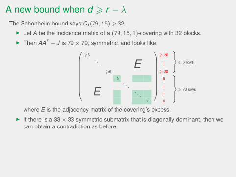
The Schonheim bound says C1(79, 15) > 32.I Let A be the incidence matrix of a (79, 15, 1)-covering with 32 blocks.I Then AAT − J is 79× 79, symmetric, and looks like
>6
> 206 6 rows. . . E ...
>6 > 20
5 6> 73 rows
. . . ...E . . . ...
5 6
where E is the adjacency matrix of the covering’s excess.I If there is a 33× 33 symmetric submatrix that is diagonally dominant, then we
can obtain a contradiction as before.I Such a submatrix corresponds to a set of 33 vertices in the excess that induces
a subgraph with maximum degree less than 5.I A result of Caro and Tuza guarantees such a 5-independent set in any
multigraph with degree sequence [206, 673].
A new bound when d > r − λ
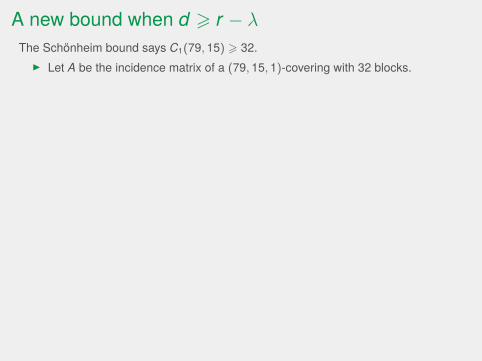
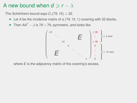
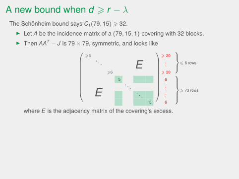
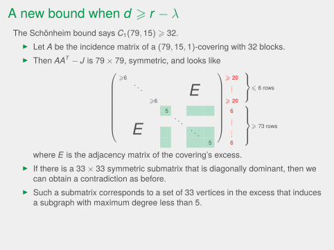
The Schonheim bound says C1(79, 15) > 32.
I Let A be the incidence matrix of a (79, 15, 1)-covering with 32 blocks.I Then AAT − J is 79× 79, symmetric, and looks like
>6
> 206 6 rows. . . E ...
>6 > 20
5 6> 73 rows
. . . ...E . . . ...
5 6
where E is the adjacency matrix of the covering’s excess.I If there is a 33× 33 symmetric submatrix that is diagonally dominant, then we
can obtain a contradiction as before.I Such a submatrix corresponds to a set of 33 vertices in the excess that induces
a subgraph with maximum degree less than 5.I A result of Caro and Tuza guarantees such a 5-independent set in any
multigraph with degree sequence [206, 673].
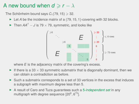
A new bound when d > r − λ
The Schonheim bound says C1(79, 15) > 32.I Let A be the incidence matrix of a (79, 15, 1)-covering with 32 blocks.
I Then AAT − J is 79× 79, symmetric, and looks like
>6
> 206 6 rows. . . E ...
>6 > 20
5 6> 73 rows
. . . ...E . . . ...
5 6
where E is the adjacency matrix of the covering’s excess.I If there is a 33× 33 symmetric submatrix that is diagonally dominant, then we
can obtain a contradiction as before.I Such a submatrix corresponds to a set of 33 vertices in the excess that induces
a subgraph with maximum degree less than 5.I A result of Caro and Tuza guarantees such a 5-independent set in any
multigraph with degree sequence [206, 673].
A new bound when d > r − λ
The Schonheim bound says C1(79, 15) > 32.I Let A be the incidence matrix of a (79, 15, 1)-covering with 32 blocks.I Then AAT − J is 79× 79, symmetric, and looks like
>6
> 206 6 rows. . . E ...
>6 > 20
5 6> 73 rows
. . . ...E . . . ...
5 6
where E is the adjacency matrix of the covering’s excess.
I If there is a 33× 33 symmetric submatrix that is diagonally dominant, then wecan obtain a contradiction as before.
I Such a submatrix corresponds to a set of 33 vertices in the excess that inducesa subgraph with maximum degree less than 5.
I A result of Caro and Tuza guarantees such a 5-independent set in anymultigraph with degree sequence [206, 673].
A new bound when d > r − λ
The Schonheim bound says C1(79, 15) > 32.I Let A be the incidence matrix of a (79, 15, 1)-covering with 32 blocks.I Then AAT − J is 79× 79, symmetric, and looks like
>6
> 206 6 rows. . . E ...
>6 > 20
5 6> 73 rows
. . . ...E . . . ...
5 6
where E is the adjacency matrix of the covering’s excess.I If there is a 33× 33 symmetric submatrix that is diagonally dominant, then we
can obtain a contradiction as before.
I Such a submatrix corresponds to a set of 33 vertices in the excess that inducesa subgraph with maximum degree less than 5.
I A result of Caro and Tuza guarantees such a 5-independent set in anymultigraph with degree sequence [206, 673].
A new bound when d > r − λ
The Schonheim bound says C1(79, 15) > 32.I Let A be the incidence matrix of a (79, 15, 1)-covering with 32 blocks.I Then AAT − J is 79× 79, symmetric, and looks like
>6
> 206 6 rows. . . E ...
>6 > 20
5 6> 73 rows
. . . ...E . . . ...
5 6
where E is the adjacency matrix of the covering’s excess.I If there is a 33× 33 symmetric submatrix that is diagonally dominant, then we
can obtain a contradiction as before.I Such a submatrix corresponds to a set of 33 vertices in the excess that induces
a subgraph with maximum degree less than 5.
I A result of Caro and Tuza guarantees such a 5-independent set in anymultigraph with degree sequence [206, 673].
A new bound when d > r − λ
The Schonheim bound says C1(79, 15) > 32.I Let A be the incidence matrix of a (79, 15, 1)-covering with 32 blocks.I Then AAT − J is 79× 79, symmetric, and looks like
>6
> 206 6 rows. . . E ...
>6 > 20
5 6> 73 rows
. . . ...E . . . ...
5 6
where E is the adjacency matrix of the covering’s excess.I If there is a 33× 33 symmetric submatrix that is diagonally dominant, then we
can obtain a contradiction as before.I Such a submatrix corresponds to a set of 33 vertices in the excess that induces
a subgraph with maximum degree less than 5.I A result of Caro and Tuza guarantees such a 5-independent set in any
multigraph with degree sequence [206, 673].
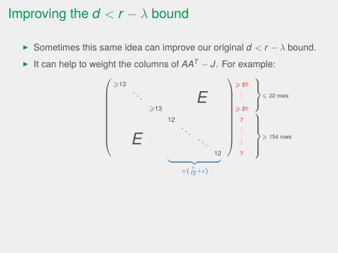
Improving the d < r − λ bound
I Sometimes this same idea can improve our original d < r − λ bound.I It can help to weight the columns of AAT − J. For example:
>13
> 216 22 rows. . . E ...
>13 > 21
12 7> 154 rows
. . ....E . . ....
12 7︸ ︷︷ ︸×( 7
12 +ε)
I We then use an edge-weighted version of the excess.I An easy extension of the Caro-Tuza result covers edge-weighted
multigraphs.

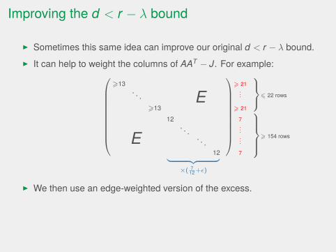
Improving the d < r − λ bound
I Sometimes this same idea can improve our original d < r − λ bound.
I It can help to weight the columns of AAT − J. For example:
>13
> 216 22 rows. . . E ...
>13 > 21
12 7> 154 rows
. . ....E . . ....
12 7︸ ︷︷ ︸×( 7
12 +ε)
I We then use an edge-weighted version of the excess.I An easy extension of the Caro-Tuza result covers edge-weighted
multigraphs.

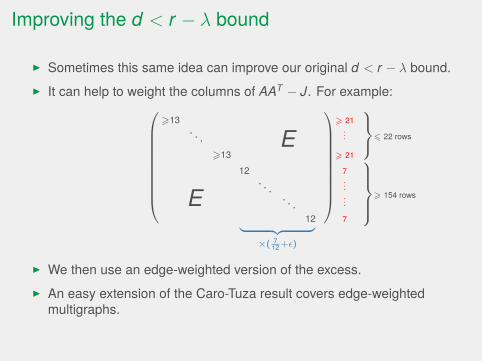
Improving the d < r − λ bound
I Sometimes this same idea can improve our original d < r − λ bound.I It can help to weight the columns of AAT − J. For example:
>13
> 216 22 rows. . . E ...
>13 > 21
12 7> 154 rows
. . ....E . . ....
12 7︸ ︷︷ ︸×( 7
12 +ε)
I We then use an edge-weighted version of the excess.I An easy extension of the Caro-Tuza result covers edge-weighted
multigraphs.
Improving the d < r − λ bound
I Sometimes this same idea can improve our original d < r − λ bound.I It can help to weight the columns of AAT − J. For example:
>13
> 216 22 rows. . . E ...
>13 > 21
12 7> 154 rows
. . ....E . . ....
12 7︸ ︷︷ ︸×( 7
12 +ε)
I We then use an edge-weighted version of the excess.
I An easy extension of the Caro-Tuza result covers edge-weightedmultigraphs.
Improving the d < r − λ bound
I Sometimes this same idea can improve our original d < r − λ bound.I It can help to weight the columns of AAT − J. For example:
>13
> 216 22 rows. . . E ...
>13 > 21
12 7> 154 rows
. . ....E . . ....
12 7︸ ︷︷ ︸×( 7
12 +ε)
I We then use an edge-weighted version of the excess.I An easy extension of the Caro-Tuza result covers edge-weighted
multigraphs.

The improvements
I These improvements produce better bounds.
I The bounds are closed form, but ugly.
I For d > r − λ we can find infinite families of improvements over theSchonheim bound.
I For d < r − λ we can find infinite families of improvements over oursimple bound.

The improvements
I These improvements produce better bounds.
I The bounds are closed form, but ugly.
I For d > r − λ we can find infinite families of improvements over theSchonheim bound.
I For d < r − λ we can find infinite families of improvements over oursimple bound.

The improvements
I These improvements produce better bounds.
I The bounds are closed form, but ugly.
I For d > r − λ we can find infinite families of improvements over theSchonheim bound.
I For d < r − λ we can find infinite families of improvements over oursimple bound.

The improvements
I These improvements produce better bounds.
I The bounds are closed form, but ugly.
I For d > r − λ we can find infinite families of improvements over theSchonheim bound.
I For d < r − λ we can find infinite families of improvements over oursimple bound.

The improvements
I These improvements produce better bounds.
I The bounds are closed form, but ugly.
I For d > r − λ we can find infinite families of improvements over theSchonheim bound.
I For d < r − λ we can find infinite families of improvements over oursimple bound.

Bounds for subsymmetric (v,15,1)-coverings
50 100 150 200 211v
new bound
Schönheim bound
0
50
100
150
200
b

Bounds for subsymmetric (v,15,1)-coverings
50 100 150 200 211v
new bound
Schönheim bound
0
50
100
150
200
b
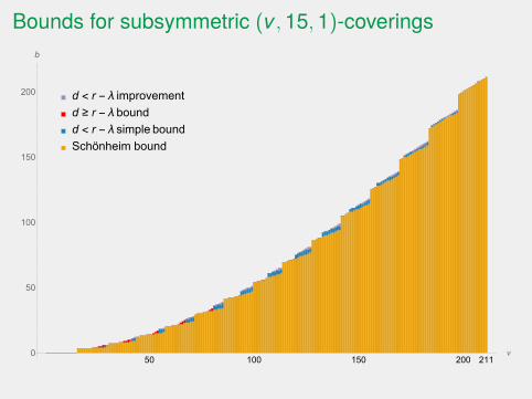
Bounds for subsymmetric (v,15,1)-coverings
50 100 150 200 211v
d < r - λ improvement
d ≥ r - λ bound
d < r - λ simple bound
Schönheim bound
0
50
100
150
200
b
Part 3Upper bounds and exact covering numbers

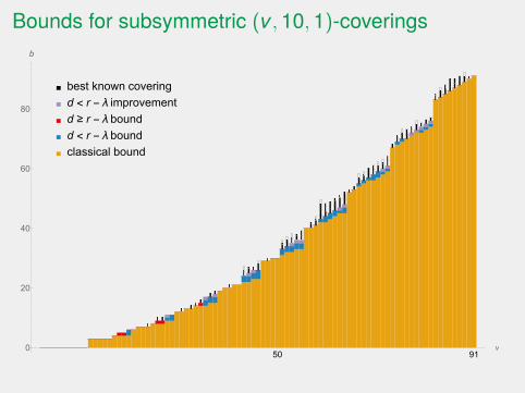
Bounds for subsymmetric (v,10,1)-coverings
50 91v
best known covering
d < r - λ improvement
d ≥ r - λ bound
d < r - λ bound
classical bound
0
20
40
60
80
b
Bounds for subsymmetric (v,10,1)-coverings
50 91v
best known covering
d < r - λ improvement
d ≥ r - λ bound
d < r - λ bound
classical bound
0
20
40
60
80
b

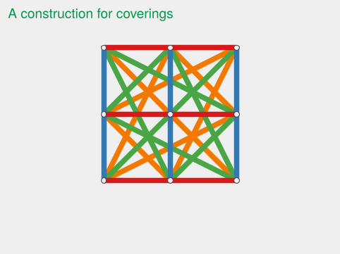
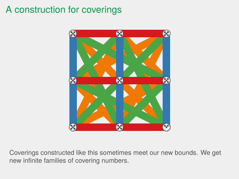
A construction for coverings
Coverings constructed like this sometimes meet our new bounds. We getnew infinite families of covering numbers.
A construction for coverings
Coverings constructed like this sometimes meet our new bounds. We getnew infinite families of covering numbers.

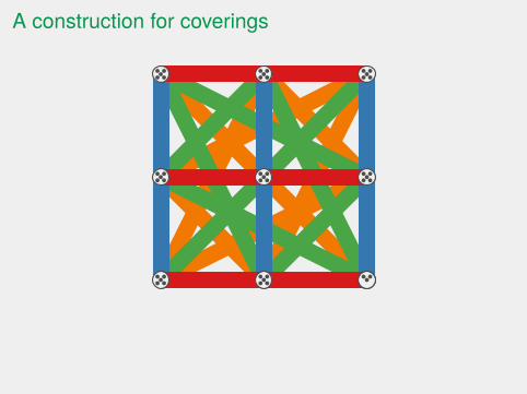
A construction for coverings
Coverings constructed like this sometimes meet our new bounds. We getnew infinite families of covering numbers.

A construction for coverings
Coverings constructed like this sometimes meet our new bounds. We getnew infinite families of covering numbers.
A construction for coverings
Coverings constructed like this sometimes meet our new bounds. We getnew infinite families of covering numbers.
A construction for coverings
Coverings constructed like this sometimes meet our new bounds. We getnew infinite families of covering numbers.
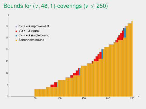
Bounds for (v,48,1)-coverings (v 6 250)
50 100 150 200 250v
d < r - λ improvement
d ≥ r - λ bound
d < r - λ simple bound
Schönheim bound
0
5
10
15
20
25
30
b
This level is exact
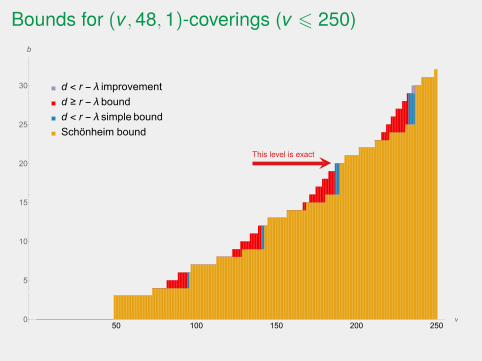
Bounds for (v,48,1)-coverings (v 6 250)
50 100 150 200 250v
d < r - λ improvement
d ≥ r - λ bound
d < r - λ simple bound
Schönheim bound
0
5
10
15
20
25
30
b
This level is exact
Bounds for (v,48,1)-coverings (v 6 250)
50 100 150 200 250v
d < r - λ improvement
d ≥ r - λ bound
d < r - λ simple bound
Schönheim bound
0
5
10
15
20
25
30
b
This level is exact
ConclusionSome final things

What about packings?
I prove very similar results for packings.
For λ = 1 these results are weaker than the second Johnson bound.
They’re still of interest for λ > 2, however.

What about packings?
I prove very similar results for packings.
For λ = 1 these results are weaker than the second Johnson bound.
They’re still of interest for λ > 2, however.

What about packings?
I prove very similar results for packings.
For λ = 1 these results are weaker than the second Johnson bound.
They’re still of interest for λ > 2, however.
What about packings?
I prove very similar results for packings.
For λ = 1 these results are weaker than the second Johnson bound.
They’re still of interest for λ > 2, however.

Further stuff
Improving these bounds:I Better results on m-independent sets in multigraphs translate immediately to
improved bounds.I With Francetic, Herke and Singh I’m working on a procedural bound for the
size of an m-independent set and on special cases where d = r − λ.
Exact covering numbers:I I’d like to find more situations in which we can construct coverings to meet
these bounds.
Symmetric coverings:I I’ve looked at these with Bryant, Buchanan, Maenhaut and Scharaschkin and
with Francetic and Herke.

Thanks.
Top Related