Communications inCommun. Math. Phys. 87, 429-447 (1982) Mathematical

Physics© Springer-Verlag 1982

Exponential Bounds and Absence of Positive Eigenvaluesfor JV-Body Schrδdinger Operators

Richard Froese*'** and Ira Herbst*'***

Institut Mittag-Leffler, Auravagen 17, S-182 62 Djursholm, Sweden

Abstract. For a large class of iV-body potentials V we prove that if ψ is aneigenfunction of — A + V with eigenvalue E then sup {α2 + E : α ̂ 0,exρ(α|x|)φeL2} is either a threshold or +oo. Consequences of this result arethe absence of positive eigenvalues and "optimal" L2-exponential lowerbounds.

I. Introduction

In this paper we will be concerned with the iV-body Schrδdinger operator

H = H0 + V, (1.1)

V= Σ Vij9 (1.2)1 ^ i < j ^ N

in Z^R^" 1 *). Here Ho arises from the operator

&o=- Σ^i/^i (1.3)

by removing the center of mass (see [16, 17] and Sect. II for more details). Each Vtj

is multiplication by a real-valued function vtj(xf — xβ, where here xeIRviV is writtenx = (x l 5..., χN). Let h0 be — A in L2(RV). We assume in what follows that each two-body potential vtj satisfies

(a) ^ . ( I + ZIQ)"1 is compact, (1.4)

(b) (l + Λ o Γ ^ ^ o K l + ^ Γ 1 i s compact. (1.5)

* Permanent address: Department of Mathematics, University of Virginia, Charlottesville,VA 22903, USA** Research in partial fulfillment of the requirements for a Ph.D. degree at the University of Virginia*** Partially supported by U.S. - N.S.F. grant MCS-81-01665

0010-3616/82/0087/0429/S03.80

430 R. Froese and I. Herbst

From (a) it easily follows that vtj is a tempered distribution. What is meant by (b) isthat the tempered distribution w^y) = y Vv^y) has the property that the sesqui-linear form Λ . r , ίiΛ . x Λ . ,A _ x 1 ,

QU )((i+h)~ 7 wf/i+ΛOΓ ^)

extends from ^(W) x 5^(RV) to the form of a compact operator on L2(RV)An important set for our purposes is the set of thresholds. To describe this set

we need further notation. Given a subset C of {1,2,..., N} with cardinality \C\ > 1,l e t H(C) = H0(C)+V(C),

V(C)= £ieCJeC

as operators in L 2 (R v ( | c | ~ 1 ) ). The operator H0{C) arises from the operator

H0(C)=-Σ

by removing the center of mass. If \C\ = 1 we define H(C) = 0.We define the set of thresholds, &~(H), associated with H as

: There exists a partition {C1? C 2,..., Ck} of{1,..., N} into fe ̂ 2 disjoint subsets, and for eachj an eigenvalue E. of ^(C^, such that E = Eγ + . . . + Ek}. (1.6)

We will also need the distance function\ l / 2

J , (1.7)

(1-8)

where |xf —R| denotes the Euclidean distance in 1RV.Our first main result is as follows:

Theorem 1.1. Suppose H = H0 + V with two-body potentials satisfying (1.4) and (1.5)above. Suppose Hψ = Eψ. Then

sup{α 2 + E : α ^

is either a threshold or + 00.

Under conditions (1.4) and (1.5) on the two-body potentials, Perry et al. [15]have shown that &~(H) is a closed countable set. We make implicit use of this factin stating a corollary of Theorem 1.1:

Corollary 1.2. Suppose H is as in Theorem i.l and Hψ = Eψ.(i) Suppose Eφ^(H) and ^{H) n [ £ , 00) is not empty. Let t0 be the first

threshold above E (more explicitly £0 = inf \βΓ{Jί) n [ £ , 00)J. Then for all

β<γto-E,2CiN-1}). (1.9)

Exponential Bounds and Absence of Positive Eigenvalues 431

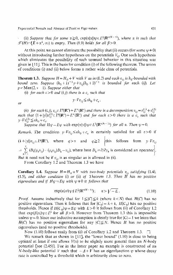
(ii) Suppose that for some α^O, Qxp(a\x\)ψe L2(W{N ~ 1]\ where a is such thatα2, oo) is empty. Then (1.9) holds for all β>0.

At this point we cannot eliminate the possibility that (ii) occurs (for some ψ Φ 0)without introducing further hypotheses on the potentials Vtj. One such hypothesiswhich eliminates the possibility of such unusual behavior in this situation wasgiven in [11]. This is the basis for condition (i) of the following theorem. The unionof conditions (i) and (ii) below forms a rather wide class of potentials.

Theorem 1.3. Suppose H = H0 + V with V as in (1.2) and each vtj is h0-bounded withbound zero. Suppose (ho + l)~1y-Vvij(ho + iy1 is bounded for each (if). Letp = Max(2, v—1). Suppose either that

(i) for each ε > 0 and (ij) there is a cε such that

or

(ii) for each (ij), vtje LP(W) + L°°(IRV) and there is a decomposition vtj = v\j] + v\fsuch that (1+ |y|)ι;jy)GLp(lRv) + L00(lRv) and for each ε > 0 there is a cε such that

Suppose that Hψ = Eψ with exp(α|x|)tpGL2(lRv(iV 1}) for all α. Then ψ = 0.

Remark. The condition y'Vvij^εh0 + cε is certainly satisfied for all ε>0 if

this follows from y VvtjO where q>v and q^V

= Σ (Dk(ykvij)~(ykvij)Dk~vij)> where here Dk = d/dyk is considered an operator I.fc=l J

But it need not be if vtj is as singular as is allowed in (ii).From Corollary 1.2 and Theorem 1.3 we have

Corollary 1.4. Suppose H = H0 + V with two-body potentials vtj satisfying (1.4),(1.5), and either condition (i) or (ii) of Theorem 13. Then H has no positiveeigenvalues and if H\p — E\p with φφO it follows that

^1'-^); α> ] / ^ £ . (1.10)

Proof Assume inductively that for l^ |C|^fe (where k<N) that H(C) has nopositive eigenvalues. Then it follows that for | C 0 | = fe+1, H{C0) has no positivethresholds. Hence if H(C0)xp = E\p with £ > 0 it follows from (ii) of Corollary 1.2that Qxp(β\x\)ψeL2 for all β>0. However from Theorem 1.3 this is impossibleunless ψ == 0. Since our inductive assumption is clearly true for \C\ = 1 we learn thatH(C) has no positive eigenvalues for any \C\^N. Hence H has no positiveeigenvalues (and no positive thresholds).

Now (1.10) follows easily from (ii) of Corollary 1.2 and Theorem 1.3. •We remark that as shown in [11], the "lower bound" (1.10) is close to being

optimal at least if one allows V(x) to be slightly more general than an JV-bodypotential [see (2.45)]. For in the latter paper an example is constructed of anN-body-like potential V such that — A + V has an eigenfunction ψ whose decayrate is controlled by a threshold which is arbitrarily close to zero.

432 R. Froese and I. Herbst

In [11], (1.10) is proved in certain important special cases including forHamiltonians which describe atomic and molecular systems. We believe that forgeneric V there are no embedded eigenvalues and that the decay rate ofeigenfunctions is controlled by the lowest threshold. A proper formulation andproof of such a result would be very interesting.

Theorem 1.3 is a kind of unique continuation theorem. We expect thatconditions (i) or (ii) of that theorem are far from optimal in eliminating arbitrarilyrapid exponential decay.

The ideas in this paper are directly descended from [11,12]. The latter paperproves absence of positive eigenvalues for a large class of one-body potentialsusing a similar method. The proof of Theorem 1.1 relies heavily on ideas from[11,12] and on the "Mourre estimate" [14] which was proved for JV-body systemsby Perry et al. [15]. The unique continuation type argument on which Theorem1.3 is based is also an extension of ideas which appear in [11,12]. Indeed undercondition (i) of that theorem, the result already appears in [11].

There are of course situations aside from those in [11,12] in which partialresults along the lines of Theorem 1.1 and Corollary 1.4 were previously known.For one-body systems of the type considered here the absence of positiveeigenvalues was proved by Kato [13], Agmon [2], and Simon [8] (see the book byEastham and Kalf [9] for further developments). For JV-body systems withpotentials dilation-analytic in angle θ o ^π/2, absence of positive eigenvalues wasknown from the work of Balslev [5] and of Simon [19]. Previous to this workWeidmann [21, 22] had used the virial theorem to prove absence of positiveeigenvalues for a class of homogeneous potentials. The work of Agmon [1] is alsorelevant here. The fact that eigenfunctions corresponding to non-thresholdeigenvalues decay exponentially (at some rate) was known for dilation-analyticpotentials from the work of Combes and Thomas [6], but as far as we are awarethe bound involving the first threshold above E is new, except of course when E isbelow the essential spectrum, in which case more detailed estimates are available[3, 7]. From the work of Agmon [3], it follows that for even more general two-body potentials, eigenfunctions with eigenvalues E < 0 must decay exponentially incertain cones even if Eeσess{H).

Some further discussion and references can be found in the notes section of[17].

The organization of this paper now follows. In Sect. II we prove a result(Theorem 2.1) from which Theorem 1.1 follows given the Mourre estimate(Theorem 2.3) of Perry et al. [15]. In Sect. Ill we prove a unique continuation typeresult (Theorem 3.1) from which Theorem 1.3 follows. Theorems 2.1, 2.3, and 3.1are given for potentials V which are more general than JV-body potentials. Theresults which generalize Theorem 1.1 and Corollary 1.4 are given in Corollaries 2.4and 3.2, respectively.

II. The Mourre Estimate and Exponential Upper Bounds

In this section we consider operators of the form

H=-A + V (2.1)

Exponential Bounds and Absence of Positive Eigenvalues 433

in L2(R"), where V is multiplication by a real-valued function satisfying

(a) Fis zl-bounded with bound less than one, (2.2)

(b) ( - A +1)~1 x - VV{~ A +1)'1 is bounded. (2.3)

Let D be the operator in L2(IR") defined by

(Df){x)=Vf(x),

and denote by A the generator of dilations:

A = (xD + D x)/2. (2.4)

We will also need the projection-valued measure {E(A): A a Borel subset of R}associated with the self-adjoint operator H.

We say that the "Mourre estimate" is satisfied at a point AoeIR if there exists anon-empty open interval A containing λ0, a constant c o > 0 and a compactoperator Ko so that

E(Δ)IH9 A] E(A) ̂ c0E(A) + Ko. (2.5)

Clearly the set of λ0 for which the Mourre estimate is satisfied is open. We denoteby S(H) the complement of the latter set. The estimate (2.5) was introduced byMourre [14] who proved that it was satisfied at non-threshold points for certain3-body Hamiltonians, and used it to prove σ s c (H) = 0. Mourre's result wasimproved and extended to iV-body Hamiltonians by Perry et al. [15] (see Theorem2.3 below).

We use the notation [iί, A] for the quantity — 2A — x VV which is a form on@(Δ) x @ι(Δ).

In this section we will prove the following result and then apply it to JV-body/ n \ l / 2

systems. We use the notation \x\ = £ xf

Theorem 2.1. Let H— — A + V in L2(1R"), where V is a real-valued functionsatisfying (2.2) and (2.3). Suppose Hψ = Eψ. Then

+ £:α>05exp(α|x|)t/;GL2(IR")}

is either + oo or in S(H).

The following lemma, which will be crucial in our proof of Theorem 2.1, wasused in [12]. We sketch a proof (different from that in [12]) in an appendix.

Lemma 2.2 Let H be as in Theorem 2.1 and Hxp = Eψ. Let ρ(x) = (|x|2 +1) 1 / 2 . Forε > 0 and λ>0 let

) = xg(x).

Let ψF = Qxp(F)ψ and define the operator

2 (2.6)

434 R. Froese and I. Herbst

Then ψFe@(A) and

ExpF, (2.7)

(ψF, HψF) = {ψF, ((VF)2 + E)ψF), (2.8)

(ψF, [fl, A]φ F ) = - 41 |0 1 / 2 ^ψ F | | 2 + (φF, {(x F ) 2 # - x • F(FF)2}y>F). (2.9)

// m addition ρλexp(αρ)φEL2(IR") /or α// A and some fixed a^O, then the above alsoholds with

λ1)

for all 7 > 0 and λ>0.

Remarks, (i) In case F = λ\n(ρ(l + ερ)~Λ), an easy calculation gives

1 . (2.10)

Although in this case we do not know that ψFe^(A), it easily follows that thefunction g1/2AxpF is in L2(IR") so that \\g1/2AψF\\ has an obvious meaning.

(ii) Note that limAln(ρ(l+ερ)"1) = Alnρ, lim (aιρ + λln{l+γρλ~ί)) = {ac + γ)ρ9£ 4 0 λ-*oo

and this is the reason for our choice of F. Clearly the lemma is also true for otherchoices. The crucial fact which makes (2.9) useful is the positivity of \\gll2AψF\\2.This is a consequence of our choice of radially symmetric, monotone increasingfunctions F. For the purpose of understanding why (2.9) can be useful, one shouldthink of the second term on the right side of (2.9) as negligible and compare (2.9)with (2.5).

(iii) Formally (2.9) follows from the equation (ψ, [H,exp(F)^4exρ(F)]φ) = 0.

Proof of Theorem 2.1. Before beginning in earnest we illustrate the strategy of theproof. Suppose Hψ = Eψ and that sup{α2 + £ : α ^ 0 , exp(α|x|)ιpeL2} = αo+ EφS'(H). Suppose for simplicity that ρAexp(αoρ)φeL2 for all λ. Then if y > 0 andF = αoρ + λln^ + yρ/l"1) we clearly have lim ||exp(F)φ|| = oo. Thus the vector Ψλ

λ-»oo

= exp(F)φ/||exp(F)φ|| leaves every compact set as A-κx). It turns out that (H — E— (VF)2)Ψλ^0 so that for small γ, Ψλ has energy concentrated around E-\-a^. If Fwere actually equal to (αo + y)|x|, then we would have (x V)2g — (x V){VF)2

= (αo + 'y)|x|~1 which contributes negligibly to (2.9) as λ-+oo. This is not far fromtrue. Since the energy of Ψλ is concentrated around E + &\ and Ψλ converges tozero weakly, the negativity oί(Ψλ, [H, A~]Ψλ) which follows from (2.9) contradictsits positively guaranteed by the Mourre estimate.

We now proceed to implement these ideas. We first show that if Eφ$(H) thenρAtpeL2(IRM) for λ>0. Assume the contrary so that for some 2>0, ρλψφL2{W). LetF = λln(ρ(l-fερ)' 1 )and

By the monotone convergence theorem, | | *F F | | 2 = j(ρ/(H-ερ))2A|ιp|2ίiMx convergesto §ρ2λ\ψ\2dnx— + oo so that for any bounded set B

l imf B | !P β |Vx = 0. (2.11)ε|0

Exponential Bounds and Absence of Positive Eigenvalues 435

By explicit calculation we find

(ΓF)2 = λ 2 ( l - ρ - 2 ) ρ - 2 ( l + ε ρ ) - 2 , (2.12)

so that \VF\ ^ λρ~ \ It follows from this, Eq. (2.8), and the fact that V is A -boundedwith bound less than 1 that || VΨε\\ is bounded as ε JO. Using this fact, it similarlyfollows from (2.6) and (2.7) that \\(-Δ + ί)Ψε\\ is bounded as εjO. Hence from(2.11), (—A + l)Ψε converges weakly to zero as ε |0 . From the compactness ofρ~ιD{-A + iyι we have as εjO

-+0.

Similarly \\{VF)2Ψε\\ and ||(D VF)Ψε\\ converge to zero so that from (2.7) we have

=O. (2.13)ε j O

By definition of S(H\ (2.5) holds for some A containing E, some c o > 0 and somecompact operator Ko. Without loss of generality we can assume A = [E — <5, E + δ]for some <5>0. Since Ψε converges weakly to zero, we thus have

lim inf (ψ& E{A)[_H, A]E(Δ)Ψε) ^ c0 lim inf \\E(A)Ψε\\2

ε|0 ε|0

= c o > 0 , (2.14)where the equality in (2.14) follows from

lim ||£(IRV1)ye|| ^l im \\{H- E)δ"xE(β\Δ)Ψe\\ε |0 εjO

^δ~ι lim \\(H-E)Ψε\\ =0. (2.15)ε|0

We now use (2.9) to derive a contradiction to (2.14). First by explicitcalculation [using (2.10) and (2.12)] we find

for some c1 independent of ε, so that from (2.9)

lim sup (ψ& IH, A] Ψε)^0, (2.16)we now claim that ε i 0

lim \\{-Δ + ί)E(R\Δ)Ψe\\ = 0 . (2.17)ε|0

To see this we use (2.13) and (2.15) to get

lim \\(H + i)E(β\Δ)Ψε\\ ^lim \\E(JR\A)(H-E)Ψεε|0 ε|0

ε | 0

which implies (2.17) because V is A -bounded with bound less than one.We have

(2.18)

436 R. Froese and I. Herbst

where

From (2.17) and (2.3) we have

(Here we have used [H,A~] = —2A — x-VV.) Similarly lim/2(ε) = 0, so that fromε | 0

(2.18) and (2.16), we havelim sup (Ψε,E(Δ)[H,A]E{Δ)Ψε) ^ 0 . (2.19)

ε|0

This contradicts (2.14) so we have shown that \ϊEφS{H\ then ρλψeL2(Rn) for all λ.Suppose now that the theorem is false so that

sup{α2 + £:exp(αρVeL2(IRn),α>0}=αJ + £ , (2.20)

where α ^ O and oc2

ί+E = Λφ£>(H). Again we know that (2.5) holds withΔ = [Λ — δ,Λ + δ~] for some <5>0, c o > 0 , and Ko compact. If α 1 = 0 , set α = α 1 = 0 . Ifα1 >0, then choose αe[0, αx) so that

(2.21)

In either case we have for all λ>0

ρAexp(αρ)ψeZ2(IRn). (2.22)

Suppose 7 > 0 is such that α + y > α r Then by (2.20) we have

(2.23)

We will obtain a contradiction for sufficiently small y >0. In the following we alsoassume ye(0,1]. Let F = ocρ + λln(l-\-yρλ~1) and ψF = exp(F)ψ, Ψλ = ψF/\\ψF\\ Asin the previous argument we conclude from (2.23) that for any bounded set

\\m$B\Ψλ\2dnx = 0. (2.24)

λ->oo

In the following we denote by bpj= 1,2,... constants which are independent of α,y, and λ. By direct computation we have

1 Γ 1 ) , (2.25)

so that\VF\^0L + y^bl9 \ΔF\^b2. (2.26)

It thus follows from (2.8) that HFίFJ Sb3- Using the latter in conjunction with(2.26) and (2.7) gives

(2.27)

Exponential Bounds and Absence of Positive Eigenvalues 437

In particular, (2.27) and (2.24) imply that (—Δ + l)Ψλ converges weakly to zero. Inaddition to (2.24) it follows easily that for any bounded set B

lim$B\VΨλ\2dnx = 0. (2.28)

λ->-oo

We claim that

lim \\(H-E-{VF)2))Ψλ\\=0. (2.29)A ^ oo

To see (2.29) note first that from (2.7)

l imsup | | ( //-£-(PF) 2 ) ϊ /

A | |= l imsup | | (D FF+P 7 F JD) ίFλ | |. (2.30)λ~* 00 λ~* 00

Since VF = xg, we find

D VF+VF D = 2gA + x-Vg9 (2.31)

and compute from (2.25)

\x Vg\ύb5ρ-1. (2.32)

From (2.30), (2.32), and (2.24) we have

. (2.33)λ->oo λ-> oo

By direct calculation and a simple estimate, we have

{x-Wg-ix-^VFΫ^bsQ-^ + yia + y)!!, (2.34)

so that from (2.9) we conclude

(ΨλXH,A\Ψλ)S-4\\gil2AΨλ\\2 + b6(Ψ^ρ-'Ψλ) + y(oc + y)/2. (2.35)

Since ( - A + \γγ\_H,A~\(-A +1)'1 is bounded, and (2.27) holds, we have

\\gU2AΨλV£b7. (2.36)From (2.32) we have

If χN is the characteristic function of {x : ρ ̂ N}9 we thus have

so that from (2.24) and (2.28) we have

Since N is arbitrarily large, lim \\gAΨλ\\ =0, so that (2.33) implies (2.29). Fromλ-> oo

(2.29) we conclude that

\imsup\\{H - E- ct2)Ψ λ\\S2ya + y2, (2.37)

438 R. Froese and I. Herbst

and thus (from (2.21))

l^\A)ΨJ^\imsup\\(H-E-a2)(2/δ)E(Έ\A)Ψλ\\

(2.38)

£ - α 2 ) l ί ' Λ | |

9 (2.39)

From (2.39) it follows that

(2.40)

From (2.5) and the fact that Ψλ converges weakly to zero we have

lim inf (<Pλ, E(Δ)\_H, A]E{Δ)Ψλ) ^ c 0 lim inf || E{Δ)Ψ}Λ-+00 λ-*oo

|2

^co(ί-(b8γ)2). (2.41)

From (2.35) however,

(2.42)λ->oo

As in previous argument (2.27), (2.40), and (2.42) imply

lim sup(<FA, E{Δ)IH9 A\E{Δ)Ψ λ) ^b12y. (2.43)

Since c0 is a fixed positive number, (2.43) contradicts (2.41) for all small enoughy > 0. Thus the theorem is proved. •

To apply Theorem 2.1 to operators of the form (1.1), let us first introduce somenotation [3]. Define the inner product

<x,y>= Σ 2 m Λ yi (2.44)

on 1RV]V. Here x = (xv ...,xN), y = {yι,.. ,yN), and x^y^ indicates the usual innerproduct in 1RV. Given a point xeRv i V, let the center of mass of x be given by

Define the subspace X C 1RV]V by

and the projections Πυ : IRviV-^lRviv

ί π Ϊ =[ ij )k 0; otherwise.

Note (Π^^mjiXi-Xjj/im^πij), (n^^m^x^ — x^m^m^. It is easy to checkthat Πij is an orthogonal projection relative to the inner product < , > and that

Exponential Bounds and Absence of Positive Eigenvalues 439

Ui X-+X. The reason that (2.44) is natural is that if

jί = l

then in fact - Ho is the Laplace-Beltrami operator for R v N with inner product< , >. In other words if we introduce an orthogonal basis {ev ..., evN} in IRvN and

vN

define the coordinates {xα: α = 1,..., vN} of a point x by writing x = Σ xαeα, thenα = 1

Removal of the center of mass motion in this language can be understood bywriting

Δ=ΔX + ΔX±,

where X®Xλ=WN and Δx is the Laplace-Beltrami operator for the subspace Xwith inner product (2.44). The operator Ho (Ho with center of mass removed) isjust — Δx so that (1.1) can be written

H=-Ax+V.

The potentials (Vij(x) = υij(xi — xJ)) clearly satisfy Vij(x)=Vij(Πijx) and thus canbe considered functions on Range Πtj CX. We are thus led to consider operators ofthe form (1.1) on L2(IR"), where

V(x)= Σ VJtΠiX). (2.45)

Here 77f is a non-zero orthogonal projection. We assume that each Vi is a real-valued function such that (denoting v ^ d i m Range I7ί? zl = Laplacian in L2(lRVί))

(a) VJί-Δi+iy1 is compact on L2(RVi). (2.46)

(b) (-Ai+ϊ)-ίyVVji-Δi+ίy1 is compact on L2(RVi). (2.47)

The statement of the Mourre estimate for these more general operatorsrequires a definition of ̂ ~(H). Let ̂ = {1,2,..., M}. For each non-empty iQJί, let

irl=[xeW:x= Σ w f w i t n uieRangeΠλ ,I iel J

and let τΓ0 = {0}. Let J^ be the family of subspaces of IR" given by

^ = {ri:lCJί). (2.48)

For ^ e # - with ^ + { 0 } 5 let

HΨ=-ΔΨ+ Σ ^ ( ^ ) , (2-49)Range ΠiCΨ

where Zlr is the Laplace operator for the subspace y and Hr is an operator inL2(IRfc) with k = dimir. If 1T is {0} we define Hr = 0 on C. We can now define

is an eigenvalue of H^ for some ' T e J ^ with iΓ + IR"} . (2.50)

440 R. Froese and I. Herbst

Theorem 1.1 follows from Theorem 2.1 and the following result (Theorem 2.3)of Perry et al. [15]. Actually in the latter paper the Mourre estimate is only anintermediate result. The authors consistently make assumptions stronger than(2.46) and (2.47) which they need in order to prove absence of singular continuousspectrum, although these stronger assumptions are not needed to prove theMourre estimate. In addition in [15] the Mourre estimate is only proved when Fisan JV-body potential of the form (1.2) and not in the more general case where V isgiven by (2.45). However the authors explicitly state that their method works forthese more general potentials with a suitable definition of thresholds. In [10] wegive an alternative (and we believe, simpler) proof of the following result:

Theorem 2.3 [15]. Suppose H=-A + Vin L2(W\ where V is given by (2.45) with Vt

real-valued multiplication operators satisfying (2.46) and (2.47). Define &~{H) by(2.50). Then ^(H) is a closed countable set and

It is not difficult to see that the set &~(H) as defined in (2.50) coincides with theset of thresholds defined in Sect. I if V is an JV-body potential of the form (1.2).

Combining Theorems 2.1 and 2.3 we have

Corollary 2.4. Suppose H is as in Theorem 2.3 and SΓ{β) is given by (2.50). Suppose

Hψ = Eψ. Then s u p { α 2 + £ :α^0,exp(αM)φeL2(R")}

is either + oo or in

We end this section with an example which shows that the Mourre estimate isvalid for more general potentials than those satisfying (2.46) and (2.47). Ourexample may seem impossible at first glance because it involves the von Neumannand Wigner [23] potential which has a positive energy bound state:

Lemma 2.5. Let H= -d2/dx2 + V(x), where V(x)=V1(x) + φinkx)/x and(a) α is real, k > 0,(b) Vί is real and V1( — d2/dx2 + l)~ί is compact,(c) {-d2/dx2 + iyί(x VV1)(-d2/dx2 + iy1 is compact

Then £(H)C{0,k2/4}. In addition if |α|<fc, then £(H)C{0}.

Proof We follow [11,12] except for one important difference. Let Ho= —d2/dx2

and suppose / is a real-valued function in C (̂1R). Then it is easily seen that(i/0 + l)(/(H)-/(H 0 )) is compact. Thus

/(£Γ)[£Γ, A] f(H) =f(H0)lH, A] f(H0) + compact

=f{H0){2H0 -{x'VV1) + φinkx)/x - fcα cosfoc)/(tf0)

= 2H0(f{H0))2 - /cα/(#0)(cos kx)f(HΌ) + compact. (2.51)

If we write p= — id/dx and coskx = (eίkx+ e~ikx)/2, we have

f(H0) coskxf(H0) = l/2{f(p2)eίkxf(p2) +f(p2)e~ίkxf(p2)} .

Since eιkxpe~ίkx = p — k, we have

f(P

2)eikxf(p2) =f(p2)f((p-k)2)eikx.

Exponential Bounds and Absence of Positive Eigenvalues 441

Suppose f(p2) = g(p), where g has support in {p : \p — po\<s or \p + po\<ε} for somep0 >0, and p0 φ fc/2. Then if ε is chosen so that ε < fc/2 and ε < \p0 — fc/2|, the readercan easily check that f(p2)f{(p-k)2) = 0. Thnsf(H0)coskxf{H0) = 0 and

/(H)[H, ^]/(H) = 2H0(f(H0))2 + compact.

If ε is small enough 2H0f(H0)2^c0f(H0)

2 for some c o > 0 , so that again using thecompactness of f(H0)

2—f(H)2 the Mourre estimate follows for positive λ0

{λo=pl). For A a compact interval contained in (— oo,0), E(A) is compact so thatfor negative λθ9 the Mourre estimate is trivial.

To prove the last statement of the Lemma, according to (2.51) it is sufficient toshow that if |α|<fc,

2HJ(H0)2 - kaf(H0) cos kxf(H0) ^ c0 f(H0)

2 (2.52)

for some c0 > 0 and some / which is 1 in an interval containing fc2/4. Supposeδe(0,1). Let χ + be the indicator function of

and χ_(x) = X + (-x).

Then with f(H0) = χ+(p) + χ_(p), we have

2H0f(H0)2 ^ ((1 - δ)2k2/2)f(H0)

2. (2.53)

We will show that

||/(H0)cosfex/(iί0)|| = l/2, (2.54)

so that from (2.53) and the fact that f(H0)2=f{H0)

2H0 f(H0)2 - kaf(H0) cos kx f(HΌ) ^ f(H0)

2((l - δ)2 (k2/2) - |fcα|/2). (2.55)

If δ is small enough (2.55) implies (2.52), so that it only remains to prove (2.54).Using χ_eikxχ+ =χ+eikxχ+ =χ_eikxχ_ =0, it is easy to see that

ikxχ_+χ_eikxχ+}. (2.56)

so that | |B | |^l/2. Clearly if χ + ιp = ψ, then Bψ = ί/2e~ikxψ and hence ||B|| = l/2.This gives (2.54). •

Corollary 2.6. Let H be as in Lemma 2.5. Then H has no positive eigenvalues exceptpossibly at k2/4. If |α| < k then H has no positive eigenvalues.

Proof. According to Theorem 2.1 and Lemma 2.5, if Hxp = Exp with £ > 0 , then if|α|<k or E + k2/4 we must have exρ(αx)ipeL2(1R) for some α>0. This contradictsTheorem II. 1 of [11] unless ψ = 0.

Remark. Results of this type have been proved by O.D.E. techniques [4, 8, 16] inthe case where |t^(x)^c(l+|x|)~1~ f i for some ε>0. In fact in [4, 16] it is shown thatif |α| >k, a positive eigenvalue can indeed occur. (With a short range potential Vl9

the borderline case |α| = fc does not produce a positive eigenvalue [4,16].)

442 R. Froese and I. Herbst

III. Exponential Lower Bounds

In this section we will consider self-adjoint operators of the form

H=-Δ + V (3.1)

in L2(IRΠ), where as in the last part of Sect. II, V is a function of the form

V(x)= Σ VjJIiX). (3.2)i = 1

Here 17ί:lRn->IRn is an orthogonal projection (with respect to the usual inner

product). We will sometimes abuse notation and consider Vt to be a function onIRVi, v. = dim(Rangel7;)>0.

We state the following result whose proof is the subject of this section. (Thefirst part of the theorem is given in [11].)

Theorem 3.1. Suppose H is of the form (3.1) and V is given by (3.2), where Vt is areal-valued measurable function. Let pf = Max(2, vf — 1). Suppose either that

(i) V is A-bounded with bound less than one, (—A + l)~1x-VV(—A + l)'1 isbounded, and for some b1 and b2 with bί<2, we have

ί 2or

(ii) for each i, V;.eLPi(Rv0 + L°°(lRv0 and there is a decomposition V^where (l + lyl^eUW^ + L^QB?') and for each ε>0, y VV}1^ -εAi + bε forsome bε.

Suppose that Hψ = Eψ with exp(α|x|)φeL2(lR") for all α. Then ψ = 0.

We refer the reader to the remark made after Theorem 1.3 for a commentabout the relationship of conditions (i) and (ii).

Proof That (i) implies the result follows from [11]. We do not repeat the proofhere although the astute reader will be able to reconstruct such a proof from whatfollows. Thus assume that (ii) holds.

For simplicity we first consider the case n^3 and indicate the necessarymodifications for n^2 later. Suppose that t/ φO and let ψ(X = exp(otr)ψ, r = \x\, anddefine ΨΛ = ψJ\\xpa\\. Then as in Lemma 2.2 we find Ψae@{H),

(3.3)

(3.4)

(3.5)

(3.6)

These equations all appear in [11]. They are not difficult to obtain from those inLemma 2.2. The singularity at r = 0 is not harmful if n ̂ 3. Taking the norm of bothsides of (3.3) gives

2. (3.7)

Exponential Bounds and Absence of Positive Eigenvalues 443

A computation shows that as a quadratic form on 3>(Δ) x 9ι(Δ)

3)r- 3 , (3.8)

Thus from (3.7), (3.8), and (3.9) it follows that

\\(-Δ-u2-E)ΨJ^\\VΨJ. (3.10)

Here we have used the fact that the matrix (Qi}) is non-negative. Let

We claim thatlim UK*:;1 | l=0 . (3.11)

Given (3.11) it follows from (3.10) that for large enough α

so that\\(-A-ot2

and thus\\KaΨa\\^2a. (3.12)

From (3.5) it follows that for all large α and some cί > 0

^Cla. (3.13)

Let W1=x VV{1\ W2 = x-VV{2\ By assumption we have -A-W2^-b forsome b. Using (3.6) and (3.13) gives

2-(Ψa,W1Ψa). (3.14)

Since from (3.12)W μoi2), (3.15)

if we can show that

(3.14) will provide a contradiction for large α. Thus we must prove (3.11) and (3.16).To see (3.11) first note that ||JS:~1I|-*O so that to prove WVJtΠfήK^W-^O, we

can assume that F;eLPι(lRVι). Since we can always write Vi=fε

Ji-gε with gεeL°°(lRVl),,<ε it suffices to show that

,,.- (3.17)α->oo

To see (3.17) we factor L2(lR") = L2(IRVί)®L2(IR"-Vι) and write

1 2 2 + α 2 ) - 1 / 2 , (3.18)

444 R. Froese and I. Herbst

where Δy is the v dimensional Laplacian in the variable y and Δ± involvesorthogonal coordinates. To prove (3.17) it thus suffices to show that for eachίe[0,oo)

^ ) ^ y + i - ^ 2 - £ : ) 2 + a 2 ) - 1 / 2 | | ^ c | | ^ | | P i , (3.19)

where c is independent of t and α and the norm on the left in (3.19) is in L2(IRVi). Toprove (3.19) we use the estimate [20]

Δ^t-^-Er + ocψ^^mjf.J^πy^, (3.20)

where ftjy) = ((\y\2 + t-a2 - E)2 + <x2y112. We claim that

I I Λ J P ^ C , (3.21)

where c! is independent of t and α for large α. Clearly once (3.21) is proved we willhave shown (3.11). To estimate | |/ ί > α | |p. we assume that t — a2 — E= — β2^ — 1.Otherwise (3.21) is easy. We have with / = /ί>α

JL/W'= ί I / W + J \f\PίdyVi. (3.22)\y\2<2βi \y\2>2β2

The first integral in (3.22) can be estimated by

00

cβv ~ι j ((x2 - β2)2 + α 2 ) " P i l 2 d x . (3.23)0

We use {x2-β2)2^β2{x-β)2, where β^l to show that (3.23) is less than

Vi'1 ] (β\x- β)2 + <x2yPit2dx^4c(βv^2l*Pi-1)] (s2 + \0 0

^ const.

The second term in (3.22) is easily shown to be bounded and hence (3.21) follows.We must now prove (3.16). Since x VVi(Πix) = (Πix)-(VVi)(Πixl it suffices to showthat

(3.24)

uniformly in ί for ί^O. Note that y- VV^ = lyD, V^)'\=D-{yVll))-{yV^))-D— V Vf1'. By our previous estimate we already know that

uniformly in ί, so we need only show that

sup | | D y ( ( - J y + ί - α 2 - £ ) 2 + α 2 ) - 1 / 2 | | < o o . (3.25)ί ^ 0 , α ^ 1

Inequality (3.25) follows from the numerical estimate

which is easy to prove. Hence the proof of Theorem 3.1 is complete in the casen>3.

Exponential Bounds and Absence of Positive Eigenvalues 445

To handle the case n^2we introduce a cutoff function ηe C°°(IRM) which is zeroin a neighborhood of x = 0 and one in a neighborhood of infinity. Assuming thatφΦO we can choose η so that ηxpή^O. Defining Ψa as before, we have

where _

By choosing the support of 1 — η sufficiently small we can arrange that

\\ga\\^xp(-δa)\\ηΨJ

for some δ>0. Since {n- l){n-3)^Wa,r-^Wa)^-c\^Wa\\2 for some c (depend-ing on η), we easily find the estimate

\\KaηΨa\\£c'aL\\ηΨa\\ (3.26)

in the same way as before. Similarly we can arrange

(ηΨa,HηΨa) = {E + a2 + 0{exp( — δa)))\\ηΨJ\2, (3.27)

and2

9 (3.28)

for some δ > 0 by choosing the support of 1 — η sufficiently small.Proceeding as before using (3.26) through (3.28) yields the result. •We give the result analogous to Corollary 1.4 for the more general potential of

the type given in (3.2) in the following corol lary:

Corollary 3.2. Suppose H = — A + V with V of the form (3.2). Suppose each V{ is realand satisfies (2.46) and (2.47). Let pi = Max(2, vf— 1). Suppose in addition that either

(i) for each ί and ε>0, y VV^y)^. —εΔi + bε for some bε,or

(ii) for each i, ^eLP l(RV l) + L°°(IRvO and there is a decomposition F = F ( 1 ) + F/2),where (1 + |y|)l/.(1)eLί?ι(IRVi) + Lc0(lRVι) and for each ε>0, yW[2)^-εΔi + bε forsome bε.

Then H has no positive eigenvalues and if Hψ = Eψ with φ + 0, it follows that

α> j / ^

The proof of this result is very similar to the proof of Corollary 1.4. Theinduction is now on the family of subspaces ^ defined in (2.48). We omit thedetails.

Appendix: Proof of Lemma 2.2

In this appendix we sketch the proof of Lemma 2.2 using a method which isdifferent from that in [11] or [12].

Let F be either of the two functions given in the lemma, and let £ = exp(F).Suppose φeCJ)(Rn). Then the following formula is not difficult to derive

(φ,ίξAξ, -Δ-]φ) = (ξφ,ίA, -Δ^ξφ)-4\\gί'2Aξφ\\2+ (ξφ,Gξφ), (A.I)

446 R. Froese and I. Herbst

where

G(χ) = (x. V)2g - x - V(VF)2. (A.2)

By definition of the distribution x VV, it is easy to see that

(-ξAξφ, Vφ)-(Vφ,ξAξφ)= -(A{ξφ), V{ξφ))-(Vξφ,A{ξφ))

= (ξφ,x VVξφ). (A.3)

Here if W is the distribution x-VV, that is

then (ξφ.X'VVζφ) means W(\ξφ\2). We have assumed that (-zJ + 1)"""1*'VV( — Δ + iyι extends to a bounded operator, so we will continue to use thenotation (/,(χ VV)f) for fe®{Δ).

Hence from (A.1) we have

-2Re(ξAξφM-E)φ) = (ξφ,lA,mξφ)-4\\gίl2Aξφ\\2 + (ξφ,Gξφ). (A.4)

Suppose F = λ\n(ρ(l +ερ)~1). Then ξ is a bounded function in C^QR") and wehave g:gconstρ~3, |G|^const, \VF\ ζconst, |zlF|^const.

Let H(F) and φ be as in the lemma. Then clearly H(F) is a closed operator on@(Δ) with C^(IR") a core. In addition H{F)ψF = EψF in the sense of distributions(ψF = ξψ), so that since C^ is a core for ί/(F) we must have ψFe@(Δ) and H(F)ψF

= ExpF as vectors in L2(W). Equation (2.8) thus follows by writing

= Re(ψF,H(F)ψF)

= (ψF(H-(VF)2)xpF).

To prove (2.9) we first note that if χ is in C^(IRn), it is easy to prove (A.4) for φ = χxp.Let χ(χ) = χm{x) = χ^x/m), where χ1 e CQ(W) is one in a neighborhood of the origin.We have

(A.5)

Clearly the right side of (A.5) converges pointwise to zero and

independent of m so by the dominated convergence theorem

lim| |( l + ρ)(tf-£)χmv>| |=0. (A.6)m->oo

It is easy to see that ||(1 +QYιξAξχm\p\\ is bounded as m-^oo so that the left side of(A.4) converges to zero. Similarly the right side converges and we obtain (2.9).

The lemma is even more easily proved with F = OLQ + λ\n{\ -\-jQλ~ι) because itfollows from the assumptions that ρkQxp(F)ψ = ρkξψ is in L2 for all fe. We firstrewrite

(ξAξφ, (H - E)φ) = {Aξφ, (H(F) - E)ξφ).

Exponential Bounds and Absence of Positive Eigenvalues 447

It follows as above that ψFe!3(Δ) and (H(F) — E)ψF = 0. Using the same approxi-mation scheme as above, it follows that (H(F) — E)χmψF->0 and ΛχmψF is bounded(the latter because it easily follows that ρkAψFeL2 for all k). We omit the details ofthe proof.

Acknowledgement. It is a pleasure to thank Maria and Thomas Hoffmann-Ostenhof who firstemphasized the importance of exponential lower bounds of the type (1.10). The hospitality andfinancial support of the Mittag-Leffler Institute is also gratefully acknowledged.

References

1. Agmon, S.: Proceedings of the Int. Conf. on Funct. Anal, and Related Topics. Tokyo: Universityof Tokyo Press 1969

2. Agmon, S.: J. Anal. Math. 23, 1-25 (1970)3. Agmon, S.: Lectures on exponential decay of solutions of second order elliptic equations. Bounds

on eigenfunctions of iV-body Schrodinger operators (to be published)4. Atkinson, R : Ann. Mat. Pure Appl. 37, 347-378 (1954)5. Balslev, E.: Arch. Rat. Mech. Anal. 59, 4, 343-357 (1975)6. Combes, J.M., Thomas, L.: Commun. Math. Phys. 34, 251-270 (1973)7. Deift, P , Hunziker, W., Simon, B., Vock, E.: Commun. Math. Phys. 64, 1-34 (1978)8. Dollard, J., Friedman, C : J. Math. Phys. 18, 1598-1607 (1977)9. Eastham, M.S.P., Kalf, H.: Schrodinger type operators with continuous spectra. London: Pitman

Research Notes Series (to be published)10. Froese, R., Herbst, I.: A new proof of the Mourre estimate. Duke Math. J. (to appear)11. Froese, R., Herbst, I., Hoffmann-Ostenhof, M., Hoffmann-Ostenhof, T.: L2-exponential lower

bounds for solutions to the Schrodinger equation. Commun. Math. Phys. (to appear)12. Froese, R., Herbst, I., Hoffmann-Ostenhof, M., Hoffmann-Ostenhof, T.: On the absence of positive

eigenvalues for one-body Schrodinger operators. J. Anal. Math, (to appear)13. Kato, T.: Commun. Pure Appl. Math. 12, 403-425 (1959)14. Mourre, E.: Commun. Math. Phys. 78, 391-408 (1981)15. Perry, P., Sigal, I.M., Simon, B.: Ann. Math. 114, 519-567 (1981)16. Reed, M., Simon, B.: Methods of modern mathematical physics. III. Scattering theory. New York:

Academic Press 197917. Reed, M., Simon, B.: Methods of modern mathematical physics. IV. Analysis of operators. New

York: Academic Press 1978

18. Simon, B.19. Simon, B.20. Simon, B.

Commun. Pure Appl. Math. 22, 531-538 (1969)Math. Ann. 207, 133-138 (1974)Trace ideals and their applications. Cambridge: Cambridge University Press 1979

21. Weidmann, J.: Commun. Pure Appl. Math. 19, 107-110 (1966)22. Weidmann, J.: Bull. Am. Math. Soc. 73, 452-456 (1967)23. Von Neumann, J., Wigner, E.P.: Z. Phys. 30, 465-467 (1929)

Communicated by B. Simon

Received August 10, 1982