EXAM IN STATISTICAL MACHINE LEARNINGSTATISTISK MASKININLÄRNING

DATE AND TIME: March 10, 2017, 8.00–13.00

RESPONSIBLE TEACHER: Fredrik Lindsten

NUMBER OF PROBLEMS: 5

AIDING MATERIAL: Calculator, mathematical handbooks

PRELIMINARY GRADES: grade 3 23 pointsgrade 4 33 pointsgrade 5 43 points

Some general instructions and information:• Your solutions can be given in Swedish or in English.

• Only write on one page of the paper.

• Write your exam code and a page number on all pages.

• Do not use a red pen.

• Use separate sheets of paper for the different problems (i.e. the num-bered problems, 1–5).

• When asked to pair e.g. plots with corresponding formulas, the orderof the plots/formulas is always randomly generated using the functionsample(n) in R, where n is the number of options. Thus, it is notpossible to infer the correct answer from the way in which the problemis presented.

With the exception of Problem 1, all your answersmust be clearly motivated! A correct answer without

a proper motivation will score zero points!

Good luck!

Some useful formulas

Pages 1–3 contain some expressions that may or may not be useful for solvingthe exam problems. This is not a complete list of formulas used in thecourse! Consequently, some of the problems may require knowledge aboutcertain expressions not listed here. Furthermore, the formulas listed beloware not all self-explanatory, meaning that you need to be familiar with theexpressions to be able to interpret them. Thus, the list should be viewed as asupport for solving the problems, rather than as a comprehensive collectionof formulas.

Marginalization and conditioning of probability densities: For a par-titioned random vector Z =

(ZT

1 ZT2

)Twith joint probability density func-

tion p(z) = p(z1, z2), the marginal probability density function of Z1 is

p(z1) =∫

Z2p(z1, z2)dz2

and the conditional probability density function for Z1 given Z2 = z2 is

p(z1 | z2) = p(z1, z2)p(z2) = p(z2 | z1)p(z1)

p(z2) .

The Gaussian distribution: The probability density function of the p-dimensional Gaussian distribution is

N (x |µ, Σ) = 1(2π)p/2

√det Σ

exp(−1

2(x− µ)TΣ−1(x− µ)), x ∈ Rp.

For a Gaussian random vector X ∼ N (µ,Σ) partitioned according to,

X =(Xa

Xb

), µ =

(µaµb

), Σ =

(Σa Σab

ΣTab Σb

)

it holds that the marginal probability density of Xa is p(xa) = N (xa |µa, Σa)and the conditional density ofXa givenXb = xb is p(xa |xb) = N

(xa∣∣∣µa|b, Σa|b

),

where

µa|b = µa + ΣabΣ−1b (xb − µb),

Σa|b = Σa − ΣabΣ−1b ΣT

ab.

1

If we have that Xa, as well as Xb conditioned on Xa = xa, are Gaussiandistributed according to

p(xa) = N (xa |µa, Σa) ,p(xb |xa) = N

(xb∣∣∣Mxa + b, Σb|a

),

where M is a matrix (of appropriate dimension) and b is a constant vector,then the joint distribution of Xa and Xb is given by

p(xa, xb) = N((

xaxb

) ∣∣∣∣∣(

µaMµa + b

),

(Σa ΣaM

T

MΣa Σb|a +MΣaMT

)).

Sum of identically distributed variables: For identically distributed ran-dom variables {Zi}ni=1 with mean µ, variance σ2 and average correlation be-tween distinct variables ρ, it holds that E

[1n

∑ni=1 Zi

]= µ and Var

(1n

∑ni=1 Zi

)=

1−ρnσ2 + ρσ2.

Linear regression and regularization:

• The least-squares estimate of β in the linear regression model Y =βTX + ε is given by βLS = (XTX)−1XTy, where

X =

xT

1...xTN

, and y =

y1...yN

.

• Ridge regression uses the regularization term λ‖β‖22 = λ

∑pj=0 β

2j . The

ridge regression estimate is βRR = (XTX + λI)−1XTy.

• LASSO uses the regularization term λ‖β‖1 = λ∑pj=0 |βj|. (The LASSO

estimate does not admit a simple closed form expression.)

• For a probabilistic linear regression model with ε ∼ N (0, σ2) and priordistribution p(β) = N (β |µ0,Σ0) the posterior distribution is p(β |y) =N (β |µN ,ΣN) with

µN = ΣN

(Σ−1

0 µ0 + σ−2XTy), ΣN =

(Σ−1

0 + σ−2XTX)−1

.

Maximum likelihood: The maximum likelihood estimate is given by βML =arg maxβ `(β) where `(β) = log p(y | β) = ∑N

i=1 log p(yi | β) is the log-likelihood

2

function (the last equality holds when the N training data points are inde-pendent).

Logistic regression: The logistic regression model uses a linear regressionfor the the log-odds. In the binary classification context we thus have

log(

Pr(Y = 1 |X)Pr(Y = 0 |X)

)= βTX.

Discriminant Analysis: The linear discriminant analysis (LDA) classifierassigns a test input X = x to class k for which,

δk(x) = xTΣ−1µk −12 µ

Tk Σ−1µk + log πk

is largest, where πk = Nk/N and µk = 1Nk

∑i:yi=k xi for k = 1, . . . , K, and

Σ = 1N−K

∑Kk=1

∑i:yi=k(xi − µk)(xi − µk)T.

For quadratic discriminant analysis (QDA) we instead use the discriminantfunctions

δk(x) = −12 log |Σk| −

12(x− µk)TΣ−1

k (x− µk) + log πk,

where Σk = 1Nk−1

∑i:yi=k(xi − µk)(xi − µk)T for k = 1, . . . , K.

Loss functions for classification:• Misclassification loss: I(y 6= G(x)).• Exponential loss: exp(−yC(x)) where G(x) = sign(C(x)).

Gaussian processes: If the function f is distributed according to a Gaus-sian process, f ∼ GP(m, k), it holds that for any arbitrary selection of inputs{x(1), x(2), . . . , x(n)} the output values f(x(1)), f(x(2)), . . . , f(x(n))} are jointlyGaussian,

f(x(1))...

f(x(n))

∼ Nm(x(1))

...m(x(n))

,k(x(1), x(1)) · · · k(x(1), x(n))

... . . . ...k(x(n), x(1)) · · · k(x(n), x(n))

,

For a Gaussian process regression model Y = f(X) + ε with f ∼ GP(m, k)and ε ∼ N (0, σ2), the prediction model is given by

f(x?) |y ∼ N(m(x?) + sT(y−m(X)), k(x?, x?)− sTk(X, x?)

),

where sT = k(x?,X)(k(X,X) + σ2IN)−1.

3

1. This problem is composed of 10 true-or-false statements. You only haveto classify these as either true or false. For this problem (only!) nomotivation is required. Each correct answer scores 1 point and eachincorrect answer scores -1 point (capped at 0 for the whole problem).

i. Regression problems have only quantitative inputs.ii. The following (so called “probit”) classifier is linear:

G(x) = I(Φ(βTx) > 0.2)

where Φ(x) =∫ x−∞N (z | 0, 1)dz is the cumulative distribution

function of the standard Gaussian distribution, I(·) is the indi-cator function, and the class labels are 0 and 1.

iii. Ensemble methods can be used to reduce both bias and variance(compared to the base model used).

iv. The input partitioning shown in Figure 1 could not have beengenerated by recursive binary splitting.

X1

X2

Figure 1: Input partitioning for Problem 1.iv.

v. The model Y = β0 + β1X1 + β0β1X2 + ε (where β0 and β1 aremodel parameters) is a linear regression model.

vi. Over-fitting for a k-NN classifier occurs when there is too muchdata, so that the k-neighborhoods become to localized in the inputspace.

4

vii. Maximum likelihood estimation is another word for least-squaresestimation.

viii. The mean-squared-error (in f(X; T ) w.r.t. f(X)) can be decom-posed into the sum of the squared model bias and the model vari-ance, i.e.

E[(f(X; T )− f(X))2] =(E[f(X; T )− f(X)

])2+ E

[(f(X; T )− E[f(X; T )]

)2].

ix. AdaBoost can use logistic regression as a base classifier.x. The k-NN classifier is sensitive to the scaling of the input variables.

(10p)

5

2. A large Swedish retailer of alcoholic beverages has asked you to build amodel for predicting the price of a wine based on various types of infor-mation, such as the wine’s chemical composition, region, etc. They havecollected a database with their data, containing the following columns:

• id – a unique identification number for each row of the database,specified as an integer value• grape – one out of 6 different grapes (e.g. Syrah, Zinfandel,

Merlot, etc.)• alcohol – percentage of alcohol in the wine, specified as a real

number between 0 and 1 (e.g. 0.135 for 13.5%)• year – production year of the wine, specified as an integer in the

range 2010–2016• region – one out of 78 different wine regions (e.g. Bordeaux,

Burgundy, Rhône, etc.)• proline – concentration of the amino acid proline in mg/l speci-

fied as an integer (typically in the range 200–2000)• timestamp – a time stamp specifying the time when the row was

entered into the database, on the format ’YYYY-MM-DD HH:MM:SS’

• price – the current price of the wine in SEK, specified as aninteger (typically in the range 80–400)

Don’t forget to clearly motivate all your answers!

(a) The customer want’s to try a simple model first, like a linearregression or a logistic regression. Which one of these two methodsdo you suggest? (1p)

(b) For each column of the customer’s database as listed above, specifywhether you would consider that variable as an input of the model,an output of the model, or neither. (4p)

(c) For each of the inputs and outputs of your model (from the pre-vious question), specify whether that variable is best viewed asquantitative or qualitative. (3p)

(d) The customer has previously tried to use a CART1 model for thisproblem, but ran into problems when trying to learn this model.In fact, they were not able to train the CART model at all! The

1CART=Classification And Regression Trees

6

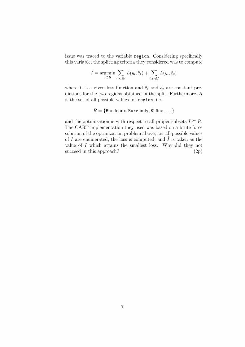
issue was traced to the variable region. Considering specificallythis variable, the splitting criteria they considered was to compute

I = arg minI⊂R

∑i:xi∈I

L(yi, c1) +∑i:xi /∈I

L(yi, c2)

where L is a given loss function and c1 and c2 are constant pre-dictions for the two regions obtained in the split. Furthermore, Ris the set of all possible values for region, i.e.

R = {Bordeaux, Burgundy, Rhône, . . . }

and the optimization is with respect to all proper subsets I ⊂ R.The CART implementation they used was based on a brute-forcesolution of the optimization problem above, i.e. all possible valuesof I are enumerated, the loss is computed, and I is taken as thevalue of I which attains the smallest loss. Why did they notsucceed in this approach? (2p)

7

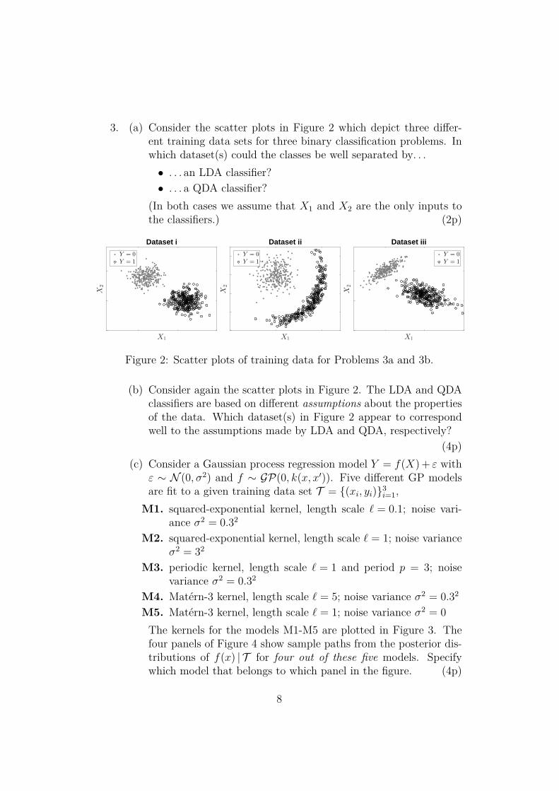
3. (a) Consider the scatter plots in Figure 2 which depict three differ-ent training data sets for three binary classification problems. Inwhich dataset(s) could the classes be well separated by. . .• . . . an LDA classifier?• . . . a QDA classifier?

(In both cases we assume that X1 and X2 are the only inputs tothe classifiers.) (2p)

X1

X2

Dataset i

Y = 0

Y = 1

X1

X2

Dataset ii

Y = 0

Y = 1

X1

X2

Dataset iii

Y = 0

Y = 1

Figure 2: Scatter plots of training data for Problems 3a and 3b.

(b) Consider again the scatter plots in Figure 2. The LDA and QDAclassifiers are based on different assumptions about the propertiesof the data. Which dataset(s) in Figure 2 appear to correspondwell to the assumptions made by LDA and QDA, respectively?

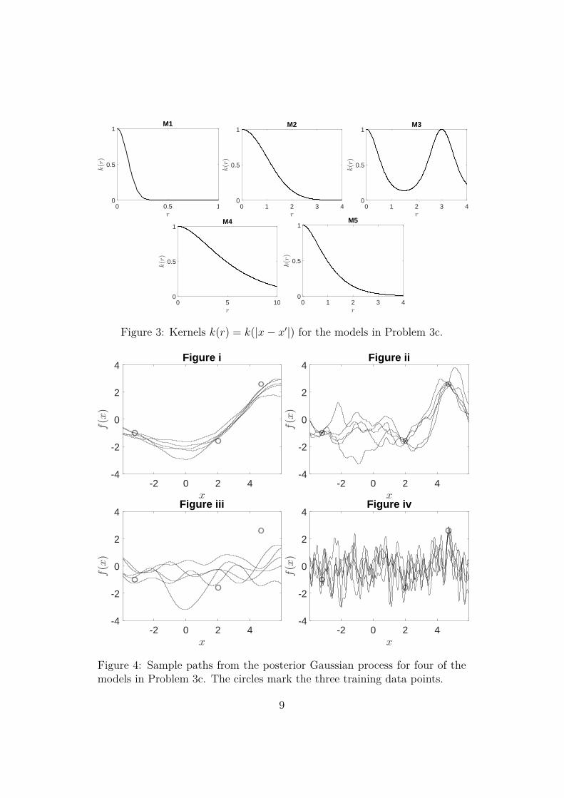
(4p)(c) Consider a Gaussian process regression model Y = f(X) + ε with

ε ∼ N (0, σ2) and f ∼ GP(0, k(x, x′)). Five different GP modelsare fit to a given training data set T = {(xi, yi)}3

i=1,M1. squared-exponential kernel, length scale ` = 0.1; noise vari-

ance σ2 = 0.32

M2. squared-exponential kernel, length scale ` = 1; noise varianceσ2 = 32

M3. periodic kernel, length scale ` = 1 and period p = 3; noisevariance σ2 = 0.32

M4. Matérn-3 kernel, length scale ` = 5; noise variance σ2 = 0.32

M5. Matérn-3 kernel, length scale ` = 1; noise variance σ2 = 0The kernels for the models M1-M5 are plotted in Figure 3. Thefour panels of Figure 4 show sample paths from the posterior dis-tributions of f(x) | T for four out of these five models. Specifywhich model that belongs to which panel in the figure. (4p)

8

0 0.5 1r

0

0.5

1

k(r)

M1

0 1 2 3 4r

0

0.5

1

k(r)

M2

0 1 2 3 4r

0

0.5

1

k(r)

M3

0 5 10r

0

0.5

1

k(r)

M4

0 1 2 3 4r

0

0.5

1

k(r)

M5

Figure 3: Kernels k(r) = k(|x− x′|) for the models in Problem 3c.

-2 0 2 4x

-4

-2

0

2

4

f(x)

Figure i

-2 0 2 4x

-4

-2

0

2

4

f(x)

Figure ii

-2 0 2 4x

-4

-2

0

2

4

f(x)

Figure iii

-2 0 2 4x

-4

-2

0

2

4

f(x)

Figure iv

Figure 4: Sample paths from the posterior Gaussian process for four of themodels in Problem 3c. The circles mark the three training data points.

9

4. (a) Consider the simple linear regression model with one input vari-able X,

Y = f(X) + ε = β0 + β1X + ε, ε ∼ N (0, σ2).

Assume that we have a training data set consisting of two datapoints T = {(x1, y1), (x2, y2)} = {(−1, 2), (1, 1)}. What is theleast-squares estimate βLS of β? (2p)

(b) What is the ridge regression estimate βRR of β? Express yoursolution in terms of the regularization parameter λ. (2p)

(c) What is the LASSO estimate βLASSO of β? Express your solutionin terms regularization parameter λ. (6p)

Hint: In two dimensions, the LASSO estimate of βj is either 0,or has the same sign as the least-squares estimate of βj. (Thisdoes not hold in higher dimensions.) Furthermore, the LASSOestimate varies continuously with λ in a piecewise linear way.

10

5. (a) Explain briefly the difference between parametric models and non-parametric models. (2p)

(b) Consider a logistic regression model for a binary classificationproblem, Y ∈ {0, 1}, with log-odds for class 1 given by βTX where

βT =(β0 β1 β2 β3

)=(3 −1 3 2

),

where the parameter β0 corresponds to an offset (“intercept”)term. According to this model, what is the probability that thetest input x? =

(2 1 −1

)belongs to class 0? (2p)

(c) Consider a logistic regression model for a binary classificationproblem Y ∈ {0, 1}. We have observed a training data set T ={(xi, yi)}Ni=1 where the N training data points are mutually inde-pendent. Write down an expression for the likelihood, i.e. theprobability of the observed training data

Pr(Y1 = y1, . . . , YN = yN |X1 = x1, . . . , XN = xN , β)

expressed in terms of the class-1 probabilities

p(x, β) := Pr(Y = 1 |X = x, β).

(4p)(d) For the logistic regression model above, write down an expression

for the log-likelihood function

`(β) = log Pr(Y1 = y1, . . . , YN = yN |X1 = x1, . . . , XN = xN , β)

on the form,

`(β) =N∑i=1

h(xi, yi, β).

The function h should be expressed only in terms of elementaryfunctions (like additions, multiplications, logarithms, exponen-tials, . . . ) and its dependence on the variables xi, yi and β shouldbe explicit. (2p)

11