

γλώσσες
Σελίδες
Νομικός

Einstein’s Theory of Gravity
February 9, 2014
Einstein’s Theory of Gravity
Newtonian Gravity
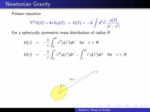
Poisson equation
∇2U(~x) = 4πGρ(~x) → U(~x) = −G∫
d3~x ′ρ(~x)
|~x − ~x ′|For a spherically symmetric mass distribution of radius R
U(r) = −1
r
∫ R
0
r ′2ρ(r ′)dr ′ for r > R
U(r) = −1
r
∫ r
0
r ′2ρ(r ′)dr ′ −∫ R
r
r ′ρ(r ′)dr ′ for r < R
Einstein’s Theory of Gravity
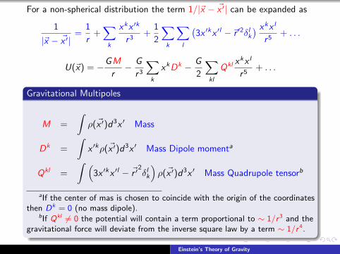
For a non-spherical distribution the term 1/|~x − ~x ′| can be expanded as
1
|~x − ~x ′|=
1
r+∑
k
xkx ′k
r3+
1
2
∑k
∑l
(3x ′kx ′l −~r ′2δl
k
) xkx l
r5+ . . .
U(~x) = −GM
r− G
r3
∑k
xkDk − G
2
∑kl
Qkl xkx l
r5+ . . .
Gravitational Multipoles
M =
∫ρ(~x ′)d3x ′ Mass
Dk =
∫x ′kρ(~x ′)d3x ′ Mass Dipole momenta
Qkl =
∫ (3x ′kx ′l − ~r ′
2δl
k
)ρ(~x ′)d3x ′ Mass Quadrupole tensorb
aIf the center of mas is chosen to coincide with the origin of the coordinatesthen Dk = 0 (no mass dipole).
bIf Qkl 6= 0 the potential will contain a term proportional to ∼ 1/r 3 and thegravitational force will deviate from the inverse square law by a term ∼ 1/r 4.
Einstein’s Theory of Gravity
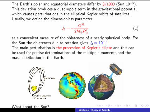
The Earth’s polar and equatorial diameters differ by 3/1000 (Sun 10−5).This deviation produces a quadrupole term in the gravitational potential,which causes perturbations in the elliptical Kepler orbits of satellites.Usually, we define the dimensionless parameter
J2 = − Q33
2MR2
(1)
as a convenient measure of the oblateness of a nearly spherical body. Forthe Sun the oblateness due to rotation gives J2 ≈ 10−7.The main perturbation is the precession of Kepler’s ellipse and this canbe used for precise determinations of the multipole moments and themass distribution in the Earth.
What about the Sun?Einstein’s Theory of Gravity
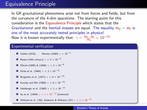
Equivalence Principle
In GR gravitational phenomena arise not from forces and fields, but fromthe curvature of the 4-dim spacetime. The starting point for thisconsideration is the Equivalence Principle which states that theGravitational and the Inertial masses are equal. The equality mG = mI isone of the most accurately tested principles in physics!Now it is known experimentally that: γ = mG−mI
mG< 10−13
Experimental verification
Galileo (1610) , Newton (1680) γ < 10−3
Bessel (19th century) γ < 2 × 10⁻⁵
Eotvos (1890) & (1908) γ < 3 × 10⁻⁹
Dicke et al. (1964) γ < 3 × 10⁻¹¹
Braginsky et al. (1971) γ < 9 × 10⁻¹³,
Kuroda and Mio (1989) γ < 8 × 10⁻¹⁰,
Adelberger et al. (1990) γ < 1 × 10⁻¹¹
Su et al. (1994) γ < 1 × 10⁻¹² (torsional)
Williams et al. (‘96), Anderson & Williams (‘01) γ < 1 × 10⁻¹³
Einstein’s Theory of Gravity
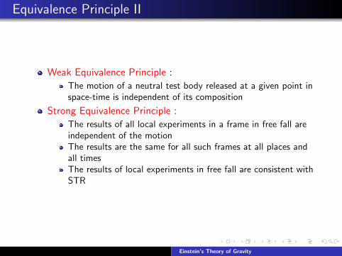
Equivalence Principle II
Weak Equivalence Principle :
The motion of a neutral test body released at a given point inspace-time is independent of its composition
Strong Equivalence Principle :
The results of all local experiments in a frame in free fall areindependent of the motionThe results are the same for all such frames at all places andall timesThe results of local experiments in free fall are consistent withSTR
Einstein’s Theory of Gravity
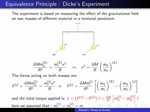
Equivalence Principle : Dicke’s Experiment
The experiment is based on measuring the effect of the gravitational fieldon two masses of different material in a torsional pendulum.
GMm(E)G
R2=
m(E)I v2
R⇒ v2 =
GM
R
(mG
mI
)(E)
The forces acting on both masses are:
F (j) +GMm
(j)G
R2=
m(j)I v2
R⇒ F (j) =
GMm(j)I
R2
[(mG
mI
)(E)
−(mG
mI
)(j)]
and the total torque applied is: L =(F (1) − F (2)
)` = GM
R2
[m
(1)G −m
(2)G
]`
here we assumed that : m(1)I = m
(2)I = m.
Einstein’s Theory of Gravity
Towards a New Theory for Gravity
Because of the success of Newton’s theory of gravity, our new theoryshould obey two demands:
In an appropriate first (weak field) approximation the new theoryshould reduce to the Newtonian one.
Beyond this approximation the new theory should predict smalldeviations from newtonian theory which must be verified byexperiments/observations
Einstein’s equivalence principle:
Gravitational and Inertial forces/accelerations are equivalent and theycannot be distinguished by any physical experiment.
This statement has 3 implications:
1 Gravitational forces/accelerations are described in the same way asthe inertial ones.
2 When gravitational accelerations are present the space cannot beflat.
3 Consequence: if gravity is present there cannot exist inertial frames.Einstein’s Theory of Gravity
1. Gravitational forces/accelerations are described in the sameway as the inertial ones.
• This means that the motion of a freely moving particle, observed
from an inertial frame, will be described by d2xµ
dt2 = 0 while from anon-inertial frame its movement will be described by the geodesicequation
d2xµ
ds2+ Γµρσ
dxρ
ds
dxσ
ds= 0 .
• The 2nd term appeared due to the use of a non-inertial frame, i.e.the inertial accelerations will be described by the Christoffel symbols.• But according to Einstein the gravitational accelerations as well willbe described by the Christoffel symbols.• This leads to the following conclusion: The metric tensor should playthe role of the gravitational potential since Γµρσ is a function of the metrictensor and its derivatives.
Einstein’s Theory of Gravity
2. When gravitational accelerations are present the space cannotbe flat
since the Christoffel symbols are non-zero and the Riemann tensor is notzero as well.In other words, the presence of the gravitational field forces the space tobe curved, i.e. there is a direct link between the presence of agravitational field and the geometry of the space.
3. Consequence: if gravity is present there cannot exist inertialframes.
If it was possible then one would have been able to discriminate amonginertial and gravitational accelerations which against the “generalizedequivalence principle” of Einstein.The absence of “special” coordinate frames (like the inertial) and theirsubstitution from “general” (non-inertial) coordinate systems lead innaming Einstein’s theory for gravity “General Theory of Relativity”.
Einstein’s Theory of Gravity
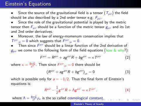
Einstein’s Equations
• Since the source of the gravitational field is a tensor (Tµν) the fieldshould be also described by a 2nd order tensor e.g. Fµν .• Since the role of the gravitational potential is played by the metrictensor then Fµν should be a function of the metric tensor gµν and its 1stand 2nd order derivatives.• Moreover, the law of energy-momenum conservation implies thatTµν
;µ = 0 which suggests that Fµν ;µ = 0.• Then since Fµν should be a linear function of the 2nd derivative ofgµν we come to the following form of the field equations (how & why?):
Fµν = Rµν + agµνR + bgµν = κTµν (2)
where κ = 8πGc4 . Then since Fµν ;µ = 0 there should be
(Rµν + agµνR + bgµν);µ = 0 (3)
which is possible only for a = −1/2. Thus the final form of Einstein’sequations is:
Rµν − 1
2gµνR + Λgµν = κTµν . (4)
where Λ = 8πGc2 ρv is the so called cosmological constant.
Einstein’s Theory of Gravity
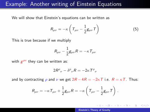
Example: Another writing of Einstein Equations
We will show that Einstein’s equations can be written as
Rµν = −κ(Tµν −
1
2gµνT
)(5)
This is true because if we multiply
Rµν −1
2gµνR = −κTµν
with gρν they can be written as:
2Rρν − δρνR = −2κT ρν
and by contracting ρ and ν we get 2R − 4R = −2κT i.e. R = κT . Thus:
Rµν = −κTµν +1
2gµνR = −κ
(Tµν −
1
2gµνT
).
Einstein’s Theory of Gravity
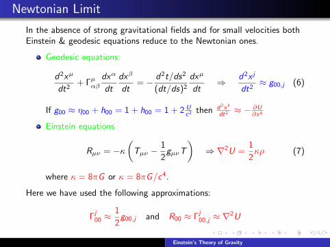
Newtonian Limit
In the absence of strong gravitational fields and for small velocities bothEinstein & geodesic equations reduce to the Newtonian ones.
Geodesic equations:
d2xµ
dt2+ Γµαβ
dxα
dt
dxβ
dt= − d2t/ds2
(dt/ds)2
dxµ
dt⇒ d2x j
dt2≈ g00,j (6)
If g00 ≈ η00 + h00 = 1 + h00 = 1 + 2 Uc2 then d2xk
dt2 ≈ − ∂U∂xk
Einstein equations
Rµν = −κ(Tµν −
1
2gµνT
)⇒ ∇2U =
1
2κρ (7)
where κ = 8πG or κ = 8πG/c4.
Here we have used the following approximations:
Γj00 ≈
1
2g00,j and R00 ≈ Γj
00,j ≈ ∇2U
Einstein’s Theory of Gravity
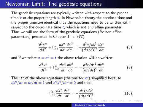
Newtonian Limit: The geodesic equations
The geodesic equations are typically written with respect to the propertime τ or the proper length s. In Newtonian theory the absolute time andthe proper time are identical thus the equations need to be written withrespect to the coordinate time t, which is not and affine parameter!Thus we will use the form of the geodesic equations (for non affineparameters) presented in Chapter 1 i.e. (??)
d2xµ
dσ2+ Γµαβ
dxα
dσ
dxβ
dσ= − d2σ/ds2
(dσ/ds)2
dxµ
dσ(8)
and if we select σ = x0 = t the above relation will be written:
d2xµ
dt2+ Γµαβ
dxα
dt
dxβ
dt= − d2t/ds2
(dt/ds)2
dxµ
dt(9)
The 1st of the above equations (the one for x0) simplified becausedx0/dt = dt/dt = 1 and d2x0/dt2 = 0 and thus
Γ0αβ
dxα
dt
dxβ
dt= − d2t/ds2
(dt/ds)2(10)
Einstein’s Theory of Gravity
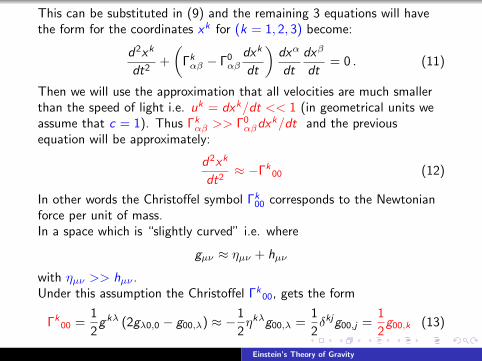
This can be substituted in (9) and the remaining 3 equations will havethe form for the coordinates xk for (k = 1, 2, 3) become:
d2xk
dt2+
(Γkαβ − Γ0
αβ
dxk
dt
)dxα
dt
dxβ
dt= 0 . (11)
Then we will use the approximation that all velocities are much smallerthan the speed of light i.e. uk = dxk/dt << 1 (in geometrical units weassume that c = 1). Thus Γk
αβ >> Γ0αβdx
k/dt and the previousequation will be approximately:
d2xk
dt2≈ −Γk
00 (12)
In other words the Christoffel symbol Γk00 corresponds to the Newtonian
force per unit of mass.In a space which is “slightly curved” i.e. where
gµν ≈ ηµν + hµν
with ηµν >> hµν .Under this assumption the Christoffel Γk
00, gets the form
Γk00 =
1
2gkλ (2gλ0,0 − g00,λ) ≈ −1
2ηkλg00,λ =
1
2δkjg00,j =
1
2g00,k (13)
Einstein’s Theory of Gravity
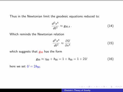
Thus in the Newtonian limit the geodesic equations reduced to:
d2xk
dt2≈ g00,k . (14)
Which reminds the Newtonian relation
d2xk
dt2≈ ∂U
∂xk(15)
which suggests that g00 has the form
g00 ≈ η00 + h00 = 1 + h00 = 1 + 2U (16)
here we set U = 2h00.
Einstein’s Theory of Gravity
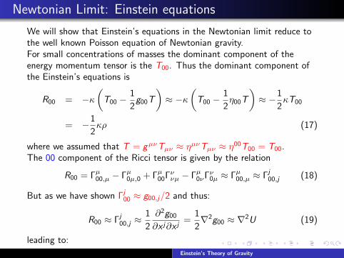
Newtonian Limit: Einstein equations
We will show that Einstein’s equations in the Newtonian limit reduce tothe well known Poisson equation of Newtonian gravity.For small concentrations of masses the dominant component of theenergy momentum tensor is the T00. Thus the dominant component ofthe Einstein’s equations is
R00 = −κ(T00 −
1
2g00T
)≈ −κ
(T00 −
1
2η00T
)≈ −1
2κT00
= −1
2κρ (17)
where we assumed that T = gµνTµν ≈ ηµνTµν ≈ η00T00 = T00.The 00 component of the Ricci tensor is given by the relation
R00 = Γµ00,µ − Γµ0µ,0 + Γµ00Γννµ − Γµ0νΓν0µ ≈ Γµ00,µ ≈ Γj00,j (18)
But as we have shown Γj00 ≈ g00,j/2 and thus:
R00 ≈ Γj00,j ≈
1
2
∂2g00
∂x j∂x j=
1
2∇2g00 ≈ ∇2U (19)
leading to:
Einstein’s Theory of Gravity
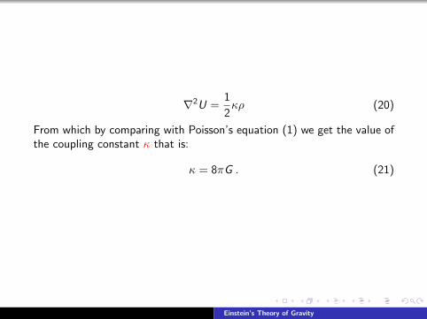
∇2U =1
2κρ (20)
From which by comparing with Poisson’s equation (1) we get the value ofthe coupling constant κ that is:
κ = 8πG . (21)
Einstein’s Theory of Gravity
Solutions of Einstein’s Equations
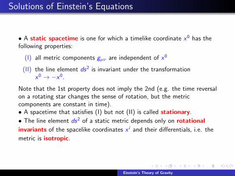
• A static spacetime is one for which a timelike coordinate x0 has thefollowing properties:
(I) all metric components gµν are independent of x0
(II) the line element ds2 is invariant under the transformationx0 → −x0.
Note that the 1st property does not imply the 2nd (e.g. the time reversalon a rotating star changes the sense of rotation, but the metriccomponents are constant in time).• A spacetime that satisfies (I) but not (II) is called stationary.
• The line element ds2 of a static metric depends only on rotational
invariants of the spacelike coordinates x i and their differentials, i.e. the
metric is isotropic.
Einstein’s Theory of Gravity
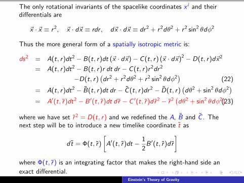
The only rotational invariants of the spacelike coordinates x i and theirdifferentials are
~x · ~x ≡ r2, ~x · d~x ≡ rdr , d~x · d~x ≡ dr2 + r2dθ2 + r2 sin2 θdφ2
Thus the more general form of a spatially isotropic metric is:
ds2 = A(t, r)dt2 − B(t, r)dt (~x · d~x)− C (t, r) (~x · d~x)2 − D(t, r)d~x2
= A(t, r)dt2 − B(t, r)r dt dr − C (t, r)r2dr2
−D(t, r)(dr2 + r2dθ2 + r2 sin2 θdφ2
)(22)
= A(t, r)dt2 − B(t, r)dt dr − C (t, r)dr2 − D(t, r)(dθ2 + sin2 θdφ2
)= A′(t, r)dt2 − B ′(t, r)dt dr − C ′(t, r)dr2 − r2
(dθ2 + sin2 θdφ2
)(23)
where we have set r2 = D(t, r) and we redefined the A, B and C . Thenext step will be to introduce a new timelike coordinate t as
dt = Φ(t, r)
[A′(t, r)dt − 1
2B ′(t, r)dr
]where Φ(t, r) is an integrating factor that makes the right-hand side an
exact differential.Einstein’s Theory of Gravity
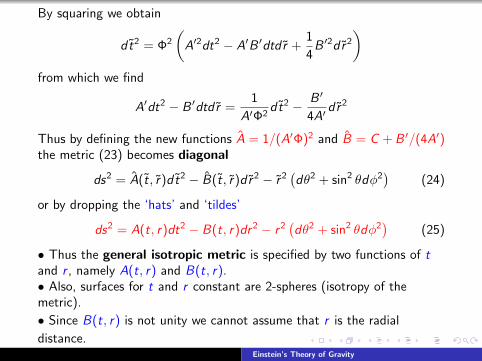
By squaring we obtain
dt2 = Φ2
(A′2dt2 − A′B ′dtdr +
1
4B ′2dr2
)from which we find
A′dt2 − B ′dtdr =1
A′Φ2dt2 − B ′
4A′dr2
Thus by defining the new functions A = 1/(A′Φ)2 and B = C + B ′/(4A′)the metric (23) becomes diagonal
ds2 = A(t, r)dt2 − B(t, r)dr2 − r2(dθ2 + sin2 θdφ2
)(24)
or by dropping the ‘hats’ and ‘tildes’
ds2 = A(t, r)dt2 − B(t, r)dr2 − r2(dθ2 + sin2 θdφ2
)(25)
• Thus the general isotropic metric is specified by two functions of tand r , namely A(t, r) and B(t, r).• Also, surfaces for t and r constant are 2-spheres (isotropy of themetric).
• Since B(t, r) is not unity we cannot assume that r is the radial
distance.Einstein’s Theory of Gravity
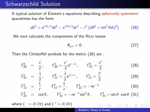
Schwarzschild Solution
A typical solution of Einstein’s equations describing spherically symmetricspacetimes has the form:
ds2 = eν(t,r)dt2 − eλ(t,r)dr2 − r2(dθ2 + sin2 θdφ2
)(26)
We next calculate the components of the Ricci tensor
Rµν = 0 . (27)
Then the Christoffel symbols for the metric (26) are :
Γ000 =
ν
2, Γ1
00 =ν′
2eν−λ , Γ0
01 =ν′
2(28)
Γ101 =
λ
2, Γ0
11 =λ
2eλ−ν , Γ1
11 =λ′
2(29)
Γ112 =
1
rΓ3
13 =1
r, Γ1
22 = −re−λ (30)
Γ323 = cot θ , Γ1
33 = −re−λ sin2 θ , Γ233 = sin θ cos θ (31)
where ( · = ∂/∂t) and ( ′ = ∂/∂r)
Einstein’s Theory of Gravity
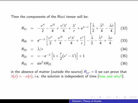
Then the components of the Ricci tensor will be:
R11 = −ν′′
2− ν′2
4+ν′λ′
4+λ′
r+ eλ−ν
[λ
2+λ2
4− λν
4
](32)
R00 = eν−λ[ν′′
2+ν′2
4− ν′λ′
4+ν′
r
]− λ
2− λ2
4+λν
4(33)
R10 = λ/r (34)
R22 = = −e−λ[1 +
r
2(ν′ − λ′)
]+ 1 (35)
R33 = sin2 θR22 (36)
in the absence of matter (outside the source) Rµν = 0 we can prove thatλ(r) = −ν(r), i.e. the solution is independent of time (how and why?).
Einstein’s Theory of Gravity
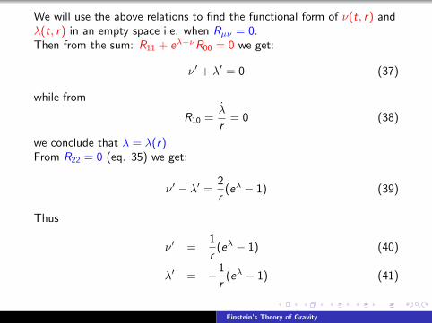
We will use the above relations to find the functional form of ν(t, r) andλ(t, r) in an empty space i.e. when Rµν = 0.Then from the sum: R11 + eλ−νR00 = 0 we get:
ν′ + λ′ = 0 (37)
while from
R10 =λ
r= 0 (38)
we conclude that λ = λ(r).From R22 = 0 (eq. 35) we get:
ν′ − λ′ =2
r(eλ − 1) (39)
Thus
ν′ =1
r(eλ − 1) (40)
λ′ = −1
r(eλ − 1) (41)
Einstein’s Theory of Gravity
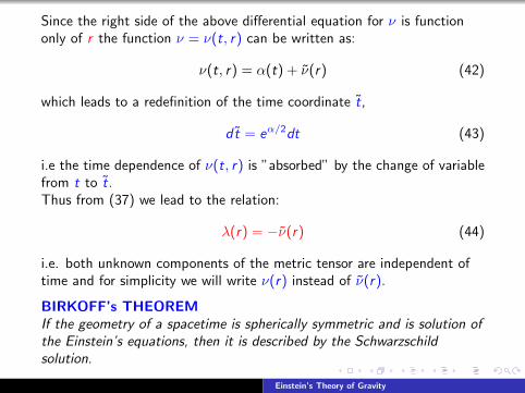
Since the right side of the above differential equation for ν is functiononly of r the function ν = ν(t, r) can be written as:
ν(t, r) = α(t) + ν(r) (42)
which leads to a redefinition of the time coordinate t,
dt = eα/2dt (43)
i.e the time dependence of ν(t, r) is ”absorbed” by the change of variablefrom t to t.Thus from (37) we lead to the relation:
λ(r) = −ν(r) (44)
i.e. both unknown components of the metric tensor are independent oftime and for simplicity we will write ν(r) instead of ν(r).
BIRKOFF’s THEOREMIf the geometry of a spacetime is spherically symmetric and is solution ofthe Einstein’s equations, then it is described by the Schwarzschildsolution.
Einstein’s Theory of Gravity
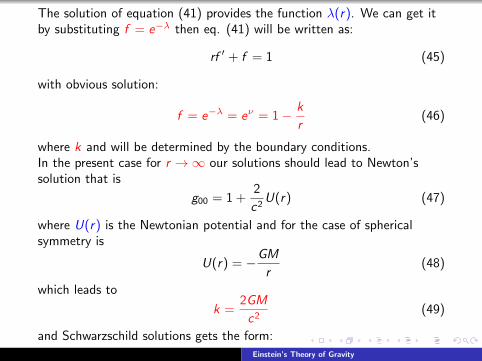
The solution of equation (41) provides the function λ(r). We can get itby substituting f = e−λ then eq. (41) will be written as:
rf ′ + f = 1 (45)
with obvious solution:
f = e−λ = eν = 1− k
r(46)
where k and will be determined by the boundary conditions.In the present case for r →∞ our solutions should lead to Newton’ssolution that is
g00 = 1 +2
c2U(r) (47)
where U(r) is the Newtonian potential and for the case of sphericalsymmetry is
U(r) = −GM
r(48)
which leads to
k =2GM
c2(49)
and Schwarzschild solutions gets the form:
Einstein’s Theory of Gravity
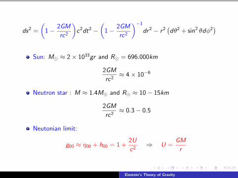
ds2 =
(1− 2GM
rc2
)c2dt2 −
(1− 2GM
rc2
)−1
dr2 − r2(dθ2 + sin2 θdφ2
)
Sun: M ≈ 2× 1033gr and R = 696.000km
2GM
rc2≈ 4× 10⁻⁶
Neutron star : M ≈ 1.4M and R ≈ 10− 15km
2GM
rc2≈ 0.3− 0.5
Neutonian limit:
g00 ≈ η00 + h00 = 1 +2U
c2⇒ U =
GM
r
Einstein’s Theory of Gravity
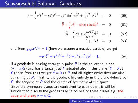
Schwarzschild Solution: Geodesics
r − 1
2ν′r2 − reν θ2 − reν sin2 θφ2 +
1
2e2νν′t2 = 0 (50)
θ +2
rr θ − sin θ cos θφ2 = 0 (51)
φ+2
rr φ+ 2
cos θ
sin θθφ = 0 (52)
t + ν′r t = 0 (53)
and from gλµxλxµ = 1 (here we assume a massive particle) we get :
−eν t2 + eλr2 + r2θ + r2 sin2 θφ2 = 1. (54)
If a geodesic is passing through a point P in the equatorial plane(θ = π/2) and has a tangent at P situated also in this plane (θ = 0 atP) then from (51) we get θ = 0 at P and all higher derivatives are alsovanishing at P. That is, the geodesic lies entirely in the plane defined byP, the tangent at P and the center of symmetry of the space.Since the symmetry planes are equivalent to each other, it will besufficient to discuss the geodesics lying on one of these planes e.g. theequatorial plane θ = π/2.
Einstein’s Theory of Gravity
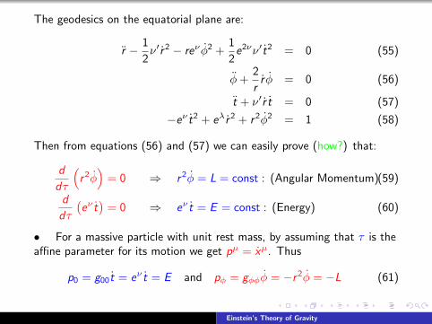
The geodesics on the equatorial plane are:
r − 1
2ν′r2 − reν φ2 +
1
2e2νν′t2 = 0 (55)
φ+2
rr φ = 0 (56)
t + ν′r t = 0 (57)
−eν t2 + eλr2 + r2φ2 = 1 (58)
Then from equations (56) and (57) we can easily prove (how?) that:
d
dτ
(r2φ)
= 0 ⇒ r2φ = L = const : (Angular Momentum)(59)
d
dτ
(eν t)
= 0 ⇒ eν t = E = const : (Energy) (60)
• For a massive particle with unit rest mass, by assuming that τ is theaffine parameter for its motion we get pµ = xµ. Thus
p0 = g00t = eν t = E and pφ = gφφφ = −r2φ = −L (61)
Einstein’s Theory of Gravity
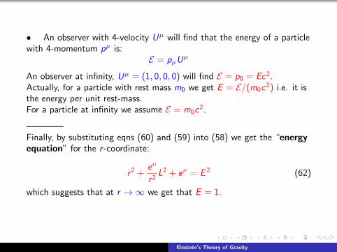
• An observer with 4-velocity Uµ will find that the energy of a particlewith 4-momentum pµ is:
E = pµUµ
An observer at infinity, Uµ = (1, 0, 0, 0) will find E = p0 = Ec2.Actually, for a particle with rest mass m0 we get E = E/(m0c
2) i.e. it isthe energy per unit rest-mass.For a particle at infinity we assume E = m0c
2.
————Finally, by substituting eqns (60) and (59) into (58) we get the “energyequation” for the r -coordinate:
r2 +eν
r2L2 + eν = E 2 (62)
which suggests that at r →∞ we get that E = 1.
Einstein’s Theory of Gravity
By combining the 2 integrals of motion and eqn (58) we can eliminate theproper time τ to derive an equation for a 3D path of the particle (how?)(
d
dφu
)2
+ u2 =E 2 − 1
L2+
2Mu
L2+ 2Mu3 (63)
where we have used u = 1/r and
r =dr
dτ=
dr
dφ
dφ
dτ=
L
r2
dr
dφ
The previous equation can be written in a form similar to Kepler’sequation of Newtonian mechanics (how?) i.e.
d2
dφ2u + u =
M
L2+ 3Mu2 (64)
The term 3Mu2 is the relativistic correction to the Newtonian equation.This term for the trajectories of planets in the solar system, whereM = M = 1.47664 km, and for orbital radius r ≈ 4.6× 10⁷km(Mercury) and r ≈ 1.5× 10⁸km (Earth) gets very small values≈ 3× 10⁻⁸ and ≈ 10−8 correspondingly.
Einstein’s Theory of Gravity
Radial motion of massive particles
For the radial motion φ is constant, which implies that L = 0 and eqn(62) reduces to
r2 = E 2 − eν (65)
and by differentiation we get an equation which reminds the equivalentone of Newtonian gravity i.e.
r =M
r2. (66)
• If a particle is dropped from the rest at r = R (r = 0) we get thatE 2 = eν(R) = 1− 2M/R and (65) will be written
r2 = 2M
(1
r− 1
R
)(67)
which is again similar to the Newtonian formula for the gain of kinetic
energy due to the loss in gravitational potential energy for a particle (of
unit mass) falling from rest at r = R.
Einstein’s Theory of Gravity
• For a particle dropped from the rest at infinity E = 1 the geodesicequations are simplified (how?):
dt
dτ= e−ν and
dr
dτ= −
√2M
r(68)
The component of the 4-velocity will be:
uµ =dxµ
dτ=
(e−ν , −
√2M
r, 0 , 0
)(69)
Then by integrating the second of (68) and by assuming that atτ = τ0 = 0 that r = r0 we get
τ =2
3
√r30
2M− 2
3
√r3
2M(70)
which suggests that for r = 0 we get τ → 23
√r 3
0
2M i.e. the particle takesfinite proper time to reach r = 0.
Einstein’s Theory of Gravity
If we want to map the trajectory of the particle in the (r , t) coordinateswe need to solve the equation
dr
dt=
dr
dτ
dτ
dt= −e−ν
√2M
r(71)
The integration leads to the relation
t =2
3
(√r30
2M−√
r3
2M
)+ 4M
(√r0
2M−√
r
2M
)
+ 2M ln
∣∣∣∣∣(√
r/2M + 1√r/2M − 1
)(√r0/2M − 1√r0/2M + 1
)∣∣∣∣∣ (72)
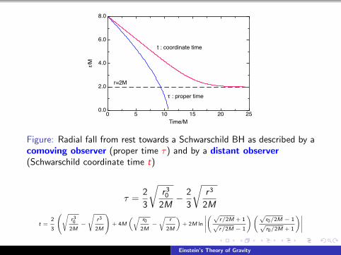
where we have chosen that for t = 0 to set r = r0.Notice that when r → 2M then t →∞. In other words, for an observerat infinity, it takes infinite time for a particle to reach r = 2M.———-
QUESTION : Can you find what will be the velocity of the radially
falling particle for a stationary observer at coordinate radius r?
Einstein’s Theory of Gravity
0 5 10 15 20 250.0
2.0
4.0
6.0
8.0
Time/M
r/M
t : coordinate time
τ : proper time
r=2M
Figure: Radial fall from rest towards a Schwarschild BH as described by acomoving observer (proper time τ) and by a distant observer(Schwarschild coordinate time t)
τ =2
3
√r30
2M− 2
3
√r3
2M
t =2
3
√ r30
2M−
√r3
2M
+ 4M
(√r0
2M−√
r
2M
)+ 2M ln
∣∣∣∣∣( √
r/2M + 1√r/2M − 1
)(√r0/2M − 1√r0/2M + 1
)∣∣∣∣∣Einstein’s Theory of Gravity
Circular motion of massive particles
The motion of massive particles in the equatorial plane is described byeqn (64)
d2
dφ2u + u =
M
L2+ 3Mu2 (73)
For circular motions r = 1/u=const and r = r = 0. Thus we get
L2 =r2M
r − 3M(74)
if we also put r = 0 in eqn (62) we get :
E =1− 2M/r√
1− 3M/r(75)
The energy of a particle with rest-mass m0 in a circular radius r is thengiven by E = E · (m0c
2).For the circular orbits to be bound we require E < m0c
2, so the limit onr for an orbit to be bound is given by E = 1 which leads to
(1− 2M/r)2 = 1− 3M/r true when r = 4M or r =∞ (76)
Thus over the range 4M < r <∞ circular orbits are bound.
Einstein’s Theory of Gravity
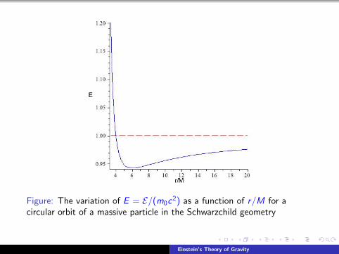
Figure: The variation of E = E/(m0c2) as a function of r/M for a
circular orbit of a massive particle in the Schwarzchild geometry
Einstein’s Theory of Gravity
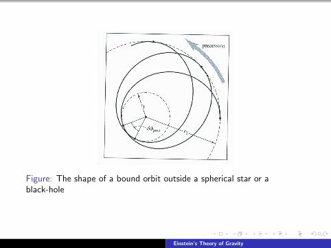
Figure: The shape of a bound orbit outside a spherical star or ablack-hole
Einstein’s Theory of Gravity
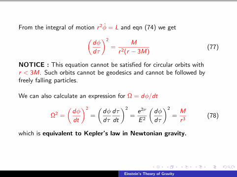
From the integral of motion r2φ = L and eqn (74) we get(dφ
dτ
)2
=M
r2(r − 3M)(77)
NOTICE : This equation cannot be satisfied for circular orbits withr < 3M. Such orbits cannot be geodesics and cannot be followed byfreely falling particles.
We can also calculate an expression for Ω = dφ/dt
Ω2 =
(dφ
dt
)2
=
(dφ
dτ
dτ
dt
)2
=e2ν
E 2
(dφ
dτ
)2
=M
r3(78)
which is equivalent to Kepler’s law in Newtonian gravity.
Einstein’s Theory of Gravity
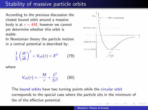
Stability of massive particle orbits
According to the previous discussion theclosest bound orbit around a massivebody is at r = 4M, however we cannotyet determine whether this orbit isstable.In Newtonian theory the particle motionin a central potential is described by:
1
2
(dr
dt
)2
+ Veff(r) = E 2 (79)
where
Veff(r) = −M
r+
L2
2r2(80)
The bound orbits have two turning points while the circular orbit
corresponds to the special case where the particle sits in the minimum of
the of the effective potential.
Einstein’s Theory of Gravity
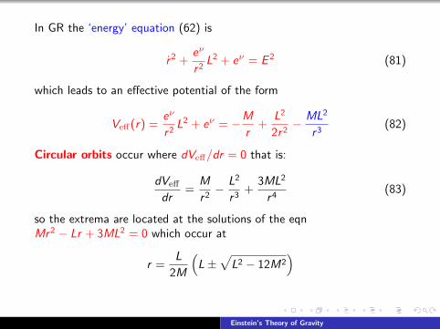
In GR the ‘energy’ equation (62) is
r2 +eν
r2L2 + eν = E 2 (81)
which leads to an effective potential of the form
Veff(r) =eν
r2L2 + eν = −M
r+
L2
2r2− ML2
r3(82)
Circular orbits occur where dVeff/dr = 0 that is:
dVeff
dr=
M
r2− L2
r3+
3ML2
r4(83)
so the extrema are located at the solutions of the eqnMr2 − Lr + 3ML2 = 0 which occur at
r =L
2M
(L±
√L2 − 12M2
)
Einstein’s Theory of Gravity
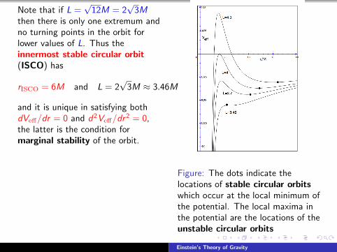
Note that if L =√
12M = 2√
3Mthen there is only one extremum andno turning points in the orbit forlower values of L. Thus theinnermost stable circular orbit(ISCO) has
rISCO = 6M and L = 2√
3M ≈ 3.46M
and it is unique in satisfying bothdVeff/dr = 0 and d2Veff/dr
2 = 0,the latter is the condition formarginal stability of the orbit.
Figure: The dots indicate thelocations of stable circular orbitswhich occur at the local minimum ofthe potential. The local maxima inthe potential are the locations of theunstable circular orbits
Einstein’s Theory of Gravity
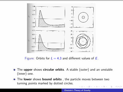
Figure: Orbits for L = 4.3 and different values of E .
The upper shows circular orbits. A stable (outer) and an unstable(inner) one.
The lower shows bound orbits , the particle moves between twoturning points marked by dotted circles.
Einstein’s Theory of Gravity
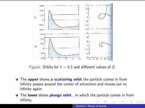
Figure: Orbits for L = 4.3 and different values of E .
The upper shows a scattering orbit the particle comes in frominfinity passes around the center of attraction and moves out toinfinity again.
The lower shows plunge orbit , in which the particle comes in frominfinity.
Einstein’s Theory of Gravity
Trajectories of photons
Photons, as any zero rest mass particle, move on null geodesics. In thiscase we cannot use the proper time τ as the parameter to characterizethe motion and thus we will use some affine parameter σ.We will study photon orbits on the equatorial plane and the equation ofmotion will be in this case
eν t = E (84)
eν t2 − e−ν r2 − r2φ2 = 0 (85)
r2φ = L (86)
The equivalent to eqn (62) for photons is
r2 +eν
r2L2 = E 2 (87)
while the equivalent of eqn (64) is
d2
dφ2u + u = 3Mu2 (88)
Einstein’s Theory of Gravity
Radial motion of photons
For radial motion φ = 0 and we get
eν t2 − e−ν r2 = 0
from which we obtain
dr
dt= ±
(1− 2M
r
)(89)
integration leads to:Outgoing Photon
t = r + 2M ln∣∣∣ r
2M− 1∣∣∣+ const
Incoming Photon
t = −r − 2M ln∣∣∣ r
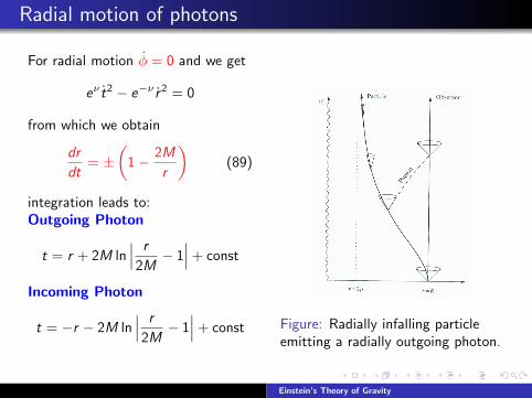
2M− 1∣∣∣+ const Figure: Radially infalling particle
emitting a radially outgoing photon.
Einstein’s Theory of Gravity
Circular motion of photons
For circular orbits we have r=constant and thus from eqn (88) we seethat the only possible radius for a circular photon orbit is:
r = 3M
(or r =
3GM
c2
)(90)
There are no such orbits around typical stars because their radius is much
larger than 3M (in geometrical units). But outside the black hole there
can be such an orbit.
Einstein’s Theory of Gravity
Stability of photon orbits
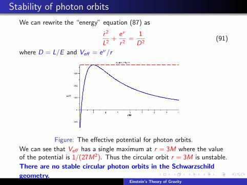
We can rewrite the “energy” equation (87) as
r2
L2+
eν
r2=
1
D2(91)
where D = L/E and Veff = eν/r
Figure: The effective potential for photon orbits.
We can see that Veff has a single maximum at r = 3M where the valueof the potential is 1/(27M2). Thus the circular orbit r = 3M is unstable.
There are no stable circular photon orbits in the Schwarzschild
geometry.Einstein’s Theory of Gravity
The slow-rotation limit : Dragging of inertial frames
ds2 = ds2Schw +
4Ma
rsin2 θdtdφ (92)
where J = Ma is the angular momentum.The contravariant components of the particles 4-momentum will be
pφ = gφµpµ = gφtpt + gφφpφ and pt = g tµpµ = g ttpt + g tφpφ
If we assume a particle with zero angular momentum, i.e. pφ = 0 alongthe geodesic then the particle’s trajectory is such that
dφ
dt=
pφ
pt=
g tφ
g tt=
2Ma
r3= ω(r)
which is the coordinate angular velocity of a zero-angular-momentumparticle.A particle dropped “straight in” from infinity ( pφ = 0) is dragged justby the influence of gravity so that acquires an angular velocity in thesame sense as that of the source of the metric.The effect weakens with the distance and makes the angularmomentum of the source measurable in practice.
Einstein’s Theory of Gravity
Useful constants
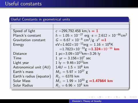
Useful Constants in geometrical units
Speed of light c =299,792.458 km/s = 1Planck’s constant ~ = 1.05× 10⁻²⁷ erg ·s = 2.612× 10−66cm2
Gravitation constant G = 6.67× 10⁻⁸ cm3/g ·s2 =1Energy eV=1.602×10⁻¹²erg = 1.16× 10⁴K
=1.7823×10⁻³³g =1.324×10−56 kmDistance 1 pc=3.09×10¹³km=3.26 lyTime 1 yr = 3.156×10⁷ secLight year 1 ly = 9.46×10¹²kmAstronomical unit (AU) 1AU = 1.5× 10⁸ kmEarth’s mass M⊕ = 5.97× 1027 gEarth’s radius (equator) R⊕ = 6378 kmSolar Mass M = 1.99× 1033 g =1.47664 kmSolar Radius R = 6.96× 10⁵ km
Einstein’s Theory of Gravity
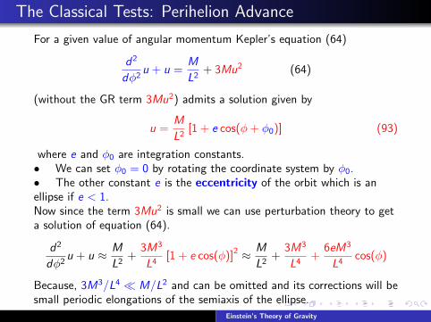
The Classical Tests: Perihelion Advance
For a given value of angular momentum Kepler’s equation (64)
d2
dφ2u + u =
M
L2+ 3Mu2 (64)
(without the GR term 3Mu2) admits a solution given by
u =M
L2[1 + e cos(φ+ φ0)] (93)
where e and φ0 are integration constants.• We can set φ0 = 0 by rotating the coordinate system by φ0.• The other constant e is the eccentricity of the orbit which is anellipse if e < 1.Now since the term 3Mu2 is small we can use perturbation theory to geta solution of equation (64).
d2
dφ2u + u ≈ M
L2+
3M3
L4[1 + e cos(φ)]2 ≈ M
L2+
3M3
L4+
6eM3
L4cos(φ)
Because, 3M3/L4 M/L2 and can be omitted and its corrections will besmall periodic elongations of the semiaxis of the ellipse.
Einstein’s Theory of Gravity
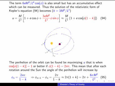
The term 6eM3/L4 cos(φ) is also small but has an accumulative effectwhich can be measured. Thus the solution of the relativistic form ofKepler’s equation (94) becomes (k = 3M2/L2)
u =M
L2
[1 + e cosφ+
3eM2
L2φ sinφ
]≈ M
L21 + e cos[φ(1− k)] (94)
The perihelion of the orbit can be found be maximizing u that is whencos[φ(1− k)] = 1 or better if φ(1− k) = 2nπ. This mean that after eachrotation around the Sun the angle of the perihelion will increase by
φn =2nπ
1− k⇒ φn+1 − φn =
2π
1− k≈ 2π(1 + k) = 2π +
6πM2
L2(95)
Einstein’s Theory of Gravity
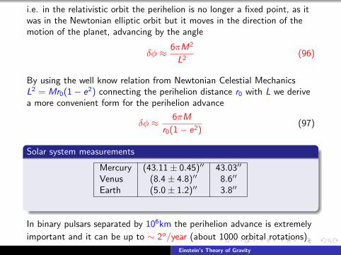
i.e. in the relativistic orbit the perihelion is no longer a fixed point, as itwas in the Newtonian elliptic orbit but it moves in the direction of themotion of the planet, advancing by the angle
δφ ≈ 6πM2
L2(96)
By using the well know relation from Newtonian Celestial MechanicsL2 = Mr0(1− e2) connecting the perihelion distance r0 with L we derivea more convenient form for the perihelion advance
δφ ≈ 6πM
r0(1− e2)(97)
Solar system measurements
Mercury (43.11± 0.45)′′ 43.03′′
Venus (8.4± 4.8)′′ 8.6′′
Earth (5.0± 1.2)′′ 3.8′′
In binary pulsars separated by 106km the perihelion advance is extremely
important and it can be up to ∼ 2o/year (about 1000 orbital rotations)
Einstein’s Theory of Gravity
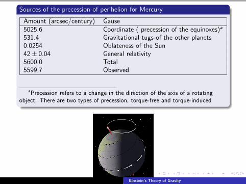
Sources of the precession of perihelion for Mercury
Amount (arcsec/century) Gause5025.6 Coordinate ( precession of the equinoxes)a
531.4 Gravitational tugs of the other planets0.0254 Oblateness of the Sun42± 0.04 General relativity5600.0 Total5599.7 Observed
aPrecession refers to a change in the direction of the axis of a rotatingobject. There are two types of precession, torque-free and torque-induced
Einstein’s Theory of Gravity
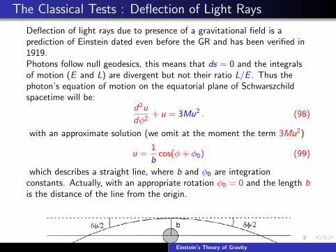
The Classical Tests : Deflection of Light Rays
Deflection of light rays due to presence of a gravitational field is aprediction of Einstein dated even before the GR and has been verified in1919.Photons follow null geodesics, this means that ds = 0 and the integralsof motion (E and L) are divergent but not their ratio L/E . Thus thephoton’s equation of motion on the equatorial plane of Schwarszchildspacetime will be:
d2u
dφ2+ u = 3Mu2 . (98)
with an approximate solution (we omit at the moment the term 3Mu2)
u =1
bcos(φ+ φ0) (99)
which describes a straight line, where b and φ0 are integrationconstants. Actually, with an appropriate rotation φ0 = 0 and the length bis the distance of the line from the origin.
Einstein’s Theory of Gravity
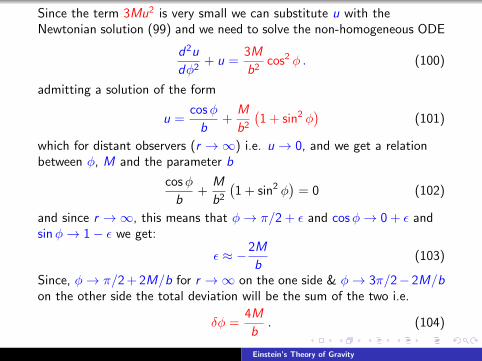
Since the term 3Mu2 is very small we can substitute u with theNewtonian solution (99) and we need to solve the non-homogeneous ODE
d2u
dφ2+ u =
3M
b2cos2 φ . (100)
admitting a solution of the form
u =cosφ
b+
M
b2
(1 + sin2 φ
)(101)
which for distant observers (r →∞) i.e. u → 0, and we get a relationbetween φ, M and the parameter b
cosφ
b+
M
b2
(1 + sin2 φ
)= 0 (102)
and since r →∞, this means that φ→ π/2 + ε and cosφ→ 0 + ε andsinφ→ 1− ε we get:
ε ≈ −2M
b(103)
Since, φ→ π/2 + 2M/b for r →∞ on the one side & φ→ 3π/2− 2M/bon the other side the total deviation will be the sum of the two i.e.
δφ =4M
b. (104)
Einstein’s Theory of Gravity
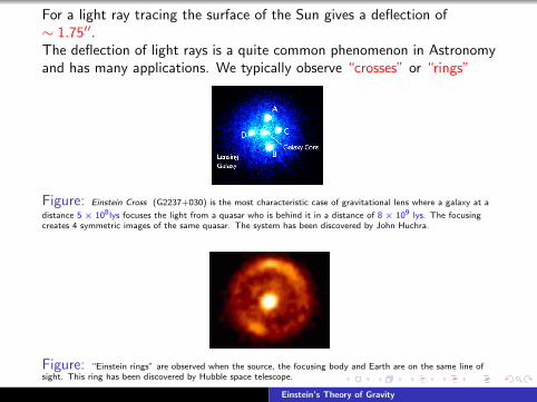
For a light ray tracing the surface of the Sun gives a deflection of∼ 1.75′′.The deflection of light rays is a quite common phenomenon in Astronomyand has many applications. We typically observe “crosses” or “rings”
Figure: Einstein Cross (G2237+030) is the most characteristic case of gravitational lens where a galaxy at a
distance 5 × 10⁸ lys focuses the light from a quasar who is behind it in a distance of 8 × 10⁹ lys. The focusingcreates 4 symmetric images of the same quasar. The system has been discovered by John Huchra.
Figure: “Einstein rings” are observed when the source, the focusing body and Earth are on the same line ofsight. This ring has been discovered by Hubble space telescope.
Einstein’s Theory of Gravity
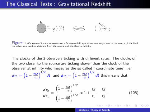
The Classical Tests : Gravitational Redshift
Figure: Let’s assume 3 static observers on a Schwarszchild spacetime, one very close to the source of the fieldthe other in a medium distance from the source and the third at infinity.
The clocks of the 3 observers ticking with different rates. The clocks ofthe two closer to the source are ticking slower than the clock of theobserver at infinity who measures the so called ‘ coordinate time” i.e.
dτ1 =(
1− 2Mr1
)1/2
dt and dτ2 =(
1− 2Mr2
)1/2
dt this means that
dτ2
dτ1=
(1− 2M
r2
)1/2
(1− 2M
r1
)1/2≈ 1 +
M
r1− M
r2. (105)
Einstein’s Theory of Gravity
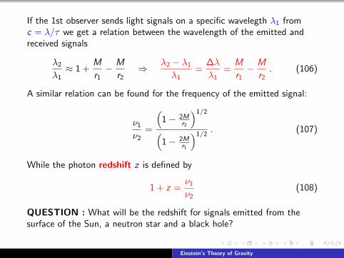
If the 1st observer sends light signals on a specific wavelegth λ1 fromc = λ/τ we get a relation between the wavelength of the emitted andreceived signals
λ2
λ1≈ 1 +
M
r1− M
r2⇒ λ2 − λ1
λ1=
∆λ
λ1=
M
r1− M
r2. (106)
A similar relation can be found for the frequency of the emitted signal:
ν1
ν2=
(1− 2M
r2
)1/2
(1− 2M
r1
)1/2. (107)
While the photon redshift z is defined by
1 + z =ν1
ν2(108)
QUESTION : What will be the redshift for signals emitted from thesurface of the Sun, a neutron star and a black hole?
Einstein’s Theory of Gravity
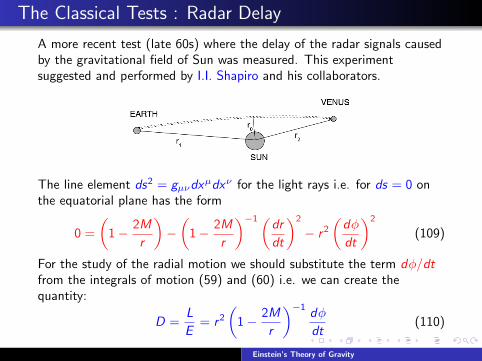
The Classical Tests : Radar Delay
A more recent test (late 60s) where the delay of the radar signals causedby the gravitational field of Sun was measured. This experimentsuggested and performed by I.I. Shapiro and his collaborators.
The line element ds2 = gµνdxµdxν for the light rays i.e. for ds = 0 on
the equatorial plane has the form
0 =
(1− 2M
r
)−(
1− 2M
r
)−1(dr
dt
)2
− r2
(dφ
dt
)2
(109)
For the study of the radial motion we should substitute the term dφ/dtfrom the integrals of motion (59) and (60) i.e. we can create thequantity:
D =L
E= r2
(1− 2M
r
)−1dφ
dt(110)
Einstein’s Theory of Gravity
Then eqn (109) becomes(1− 2M
r
)−(
1− 2M
r
)−1(dr
dt
)2
− D2
r2
(1− 2M
r
)2
= 0 . (111)
At the point of the closest approach to the Sun, r0, there should be
dr/dt = 0 and thus we get the value of D2 =r 2
0
1−2M/r0. Leading to an
equation for the radial motion:
dr
dt=
(1− 2M
r
)[1−
( r0r
)2 1− 2M/r
1− 2M/r0
]1/2
(112)
leading to
t1 =
∫ r1
r0
dr(1− 2M
r
)√1−
(r0
r
)2 1−2M/r1−2M/r0
=√
r21 − r2
0 + 2M ln
[r1√r21 − r2
0
r0
]+ M
√r1 − r0r1 + r0
≈ r1 + 2M ln
(2r1r0
)+ M
Einstein’s Theory of Gravity
For flat space we have t1 = r1 i.e. the term t1 = 2M ln(2r1/r0) + M isthe relativistic correction for the first part of the orbit in same way we geta similar contribution as the signal returns to Earth. Thus the total“extra time” is:
∆T = 2 (t1 + t2) = 4M
[1 + ln
(4r1r2r20
)]. (113)
Einstein’s Theory of Gravity
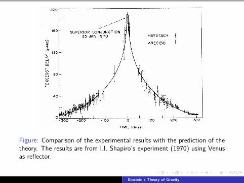
Figure: Comparison of the experimental results with the prediction of thetheory. The results are from I.I. Shapiro’s experiment (1970) using Venusas reflector.
Einstein’s Theory of Gravity
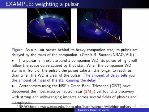
EXAMPLE: weighting a pulsar
Figure: As a pulsar passes behind its heavy companion star, its pulses aredelayed by the mass of the companion. (Credit B. Saxton/NRAO/AUI)
• If a pulsar is in orbit around a companion WD, its pulses of light willfollow the space curve caused by that star. When the companion WDstar is in front of the pulsar, the pulses take a little longer to reach usthan when the WD is clear of the pulsar. The amount of delay tells youthe amount of mass of the star causing the delay. 1
• Astronomers using the NSF’s Green Bank Telescope (GBT) have
discovered the most massive neutron star (2M) yet found, a discovery
with strong and wide-ranging impacts across several fields of physics and
astrophysics.1NRAO:http://www.nrao.edu/index.php/learn/science/weighing-pulsars
Einstein’s Theory of Gravity
Top Related