ECE 5324/6324

NOTES

ANTENNA THEORY AND DESIGN

2013

Om P. Gandhi

Text: Warren L. Stutzman and Gary A. Thiele, Antenna Theory and Design, Third Edition (2013), John Wiley & Sons. The identified page numbers and the equations with dashes (x-xxx) refer to the equations of the text.

1

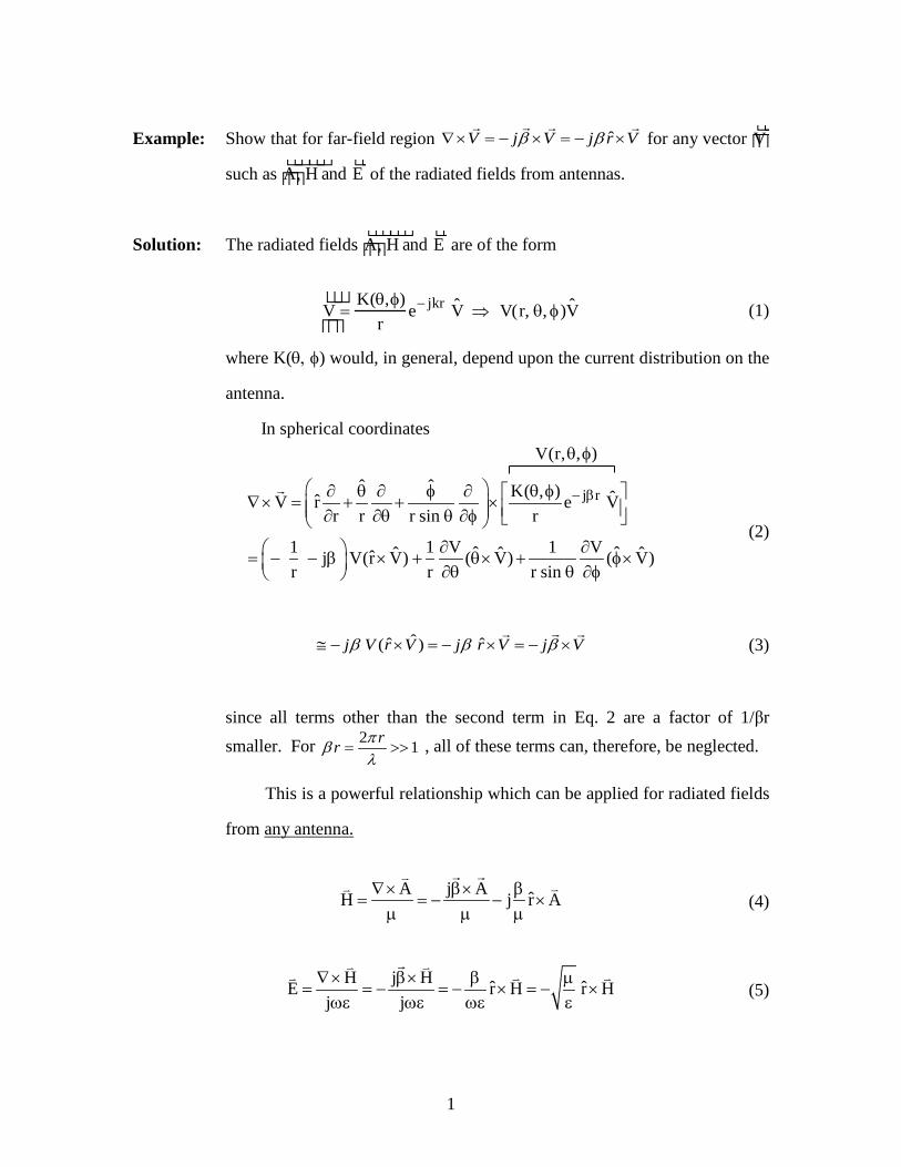
Example: Show that for far-field region ˆV j V j r Vβ β∇× = − × = − ×

for any vector V

such as A ,

H and

E of the radiated fields from antennas.

Solution: The radiated fields A ,

H and

E are of the form

V =

K(θ,φ)r

e− jkr ˆ V ⇒ V(r, θ, φ) ˆ V (1)

where K(θ, φ) would, in general, depend upon the current distribution on the

antenna.

In spherical coordinates

j rˆ ˆ K( , ) ˆˆV r e Vr r r sin r

1 1 V 1 Vˆ ˆˆ ˆ ˆˆj V(r V) ( V) ( V)r r r sin

− β ∂ θ ∂ φ ∂ θ φ ∇× = + + × ∂ ∂θ θ ∂φ ∂ ∂ = − − β × + θ× + φ× ∂θ θ ∂φ

(2)

ˆˆ ˆ( )j V r V j r V j Vβ β β≅ − × = − × = − ×

(3)

since all terms other than the second term in Eq. 2 are a factor of 1/βr smaller. For 2 1rr πβ

λ= >> , all of these terms can, therefore, be neglected.

This is a powerful relationship which can be applied for radiated fields

from any antenna.

A j A ˆH j r A∇× β× β

= = − − ×µ µ µ

(4)

H j H ˆ ˆE r H r H

j j∇× β× β µ

= = − = − × = − ×ωε ωε ωε ε

(5)

V(r, , )θ φ

2

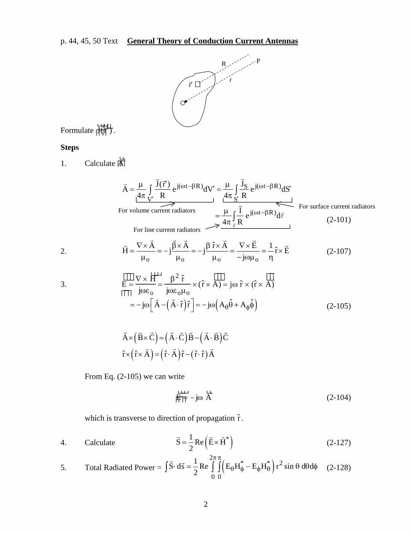
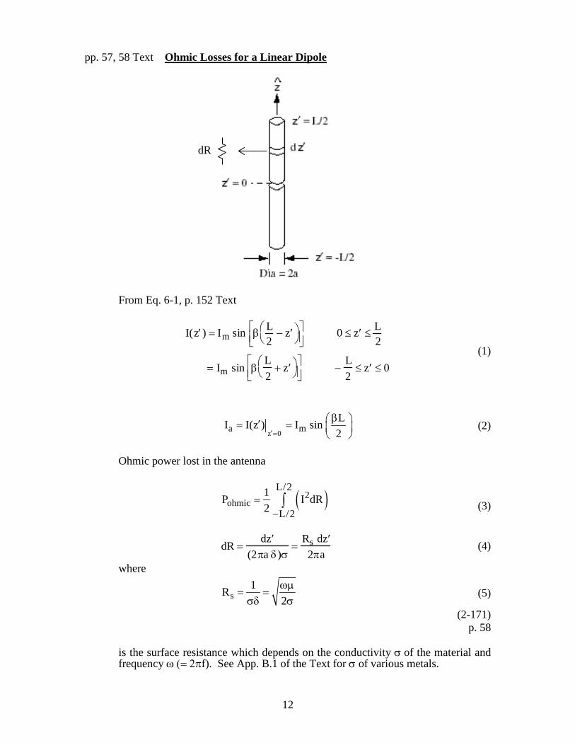
p. 44, 45, 50 Text General Theory of Conduction Current Antennas

Formulate J (

′ r ) .

Steps

1. Calculate A

j( t R) j( t R)S

V S

j( t R)

JJ(r )A e dV e dS4 R 4 R

I e d4 R

ω −β ω −β

′ ′

ω −β

′µ µ′ ′= =π π

µ=

π

∫ ∫

∫

(2-101)

2. o o o o

ˆA A r A E 1 ˆH j j r Ej

∇× β× β × ∇×= = − = − = = ×

µ µ µ − ωµ η

(2-107)

3.

E =

∇ ×H

jωεo=

β2 ˆ r jωεoµo

× (ˆ r ×A ) = jω ˆ r × (ˆ r ×

A )

( ) ( )ˆ ˆˆ ˆj A A r r j A Aθ φ = − ω − ⋅ = − ω θ + φ

(2-105)

( ) ( ) ( )

( ) ( ) ( )

A B C A C B A B C

ˆ ˆ ˆ ˆ ˆ ˆr r A r A r r r A

× × = ⋅ − ⋅

× × = ⋅ − ⋅

From Eq. (2-105) we can write

E = − jω

A (2-104)

which is transverse to direction of propagation ˆ r .

4. Calculate ( )*1S Re E H2

= ×

(2-127)

5. Total Radiated Power = ( )2

* * 2

0 0

1S ds Re E H E H r sin d d2

π π

θ φ φ θ⋅ = − θ θ φ∫ ∫ ∫

(2-128)

For volume current radiators For surface current radiators

For line current radiators

r

R

r′

P

a

Calculation of Magnetic Fields of Conduction Current Antennas Definition of Magnetic Vector Potential

A : A Simplifying Mathematical Intermediate Step

From Biot-Savart's law of electromagetism

o o2 2V

ˆ ˆI d R J dV RB4 R 4 R

′× ×= µ = µ

π π∫ ∫

oV

J dVB4 R′

′= µ ∇×

π∫

(2)

In going from Eq. 1 to Eq. 2, we have used the following steps

2

ˆ1 RR R

∇ = −

(3)

1 1 JJ J(r )R R R

′×∇ = ∇× − ∇×

(4)

The first term in Eq. 3 is zero, since the current density J

is a function of source

coordinates r (x , y , z )′ ′ ′ ′= whereas the curl J∇×

involves derivatives with respect to

field coordinates (x,y,z).

From Eq. 2

oV

J dVB A4 R′

′= µ ∇× ≡ ∇×

π∫

(5)

Thus the magnetic field at the field point can be written as curl of magnetic vector

potential A

where A

is given by

o

V

J dVA4 R′

′µ=

π ∫

(6)

Note that calculation of B

is a lot simpler if the intermediate step of first calculating A

is

undertaken since integral of Eq. 6 is much simpler than that of Eq. 5 or Eq. 1.

ˆR R R=

(x,y,z) F

I

1R

−∇

(1)

0

2

b

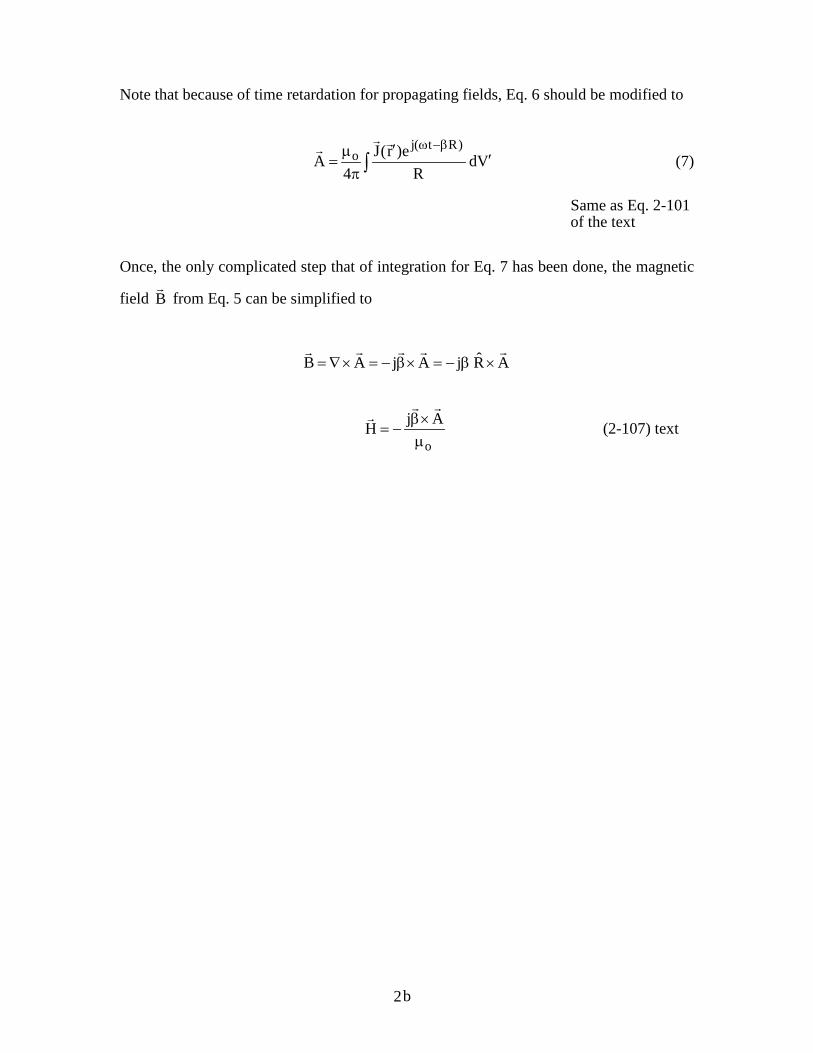
Note that because of time retardation for propagating fields, Eq. 6 should be modified to

j( t R)

o J(r )eA dV4 R

ω −β′µ ′=π ∫

(7)

Same as Eq. 2-101 of the text

Once, the only complicated step that of integration for Eq. 7 has been done, the magnetic

field B

from Eq. 5 can be simplified to

ˆB A j A j R A= ∇× = − β× = − β ×

o

j AH β×= −

µ

(2-107) text

2

3

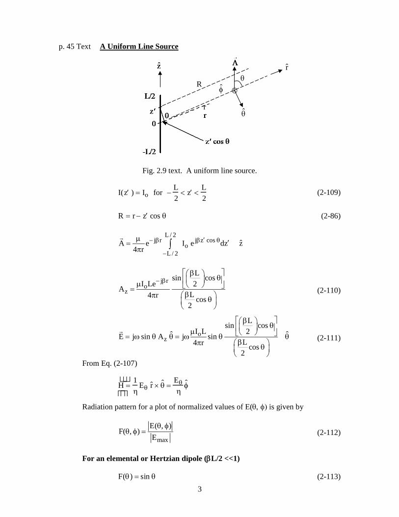
p. 45 Text A Uniform Line Source

Fig. 2.9 text. A uniform line source.

I( ′ z ) = Io for −L2

< ′ z <L2

(2-109)

R = r − ′ z cos θ (2-86)

L / 2

j r j z coso

L / 2ˆA e I e dz z

4 r′− β β θ

−

µ ′=π ∫

j r

oz

Lsin cosI Le 2A

L4 r cos2

− β β θ µ =βπ θ

(2-110)

oz

Lsin cosI L 2ˆ ˆE j sin A j sin

L4 r cos2

β θ µ = ω θ θ = ω θ θβπ θ

(2-111)

From Eq. (2-107)

H =

1η

Eθ ˆ r × ˆ θ =Eθη

ˆ φ

Radiation pattern for a plot of normalized values of E(θ, φ) is given by

max

E( , )F( , )

Eθ φ

θ φ = (2-112)

For an elemental or Hertzian dipole (βL/2 <<1) F(θ) = sin θ (2-113)

r

⊗

θ

φ R

θ

r

4

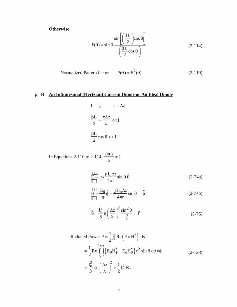
Otherwise

Lsin cos2F( ) sin

L cos2

β θ θ = θβ θ

(2-114)

Normalized Pattern factor P(θ) = F2(θ) (2-119) p. 34 An Infinitesimal (Hertzian) Current Dipole or An Ideal Dipole I = Io L = ∆z

βL2

=π∆z

λ<<1

βL2

cos θ <<1

In Equations 2-110 to 2-114; sin x

x≅ 1

E = jω

µIo∆z4πr

sin θ ˆ θ

(2-74a)

H =

Eθη

ˆ φ =jβIo∆z

4πrsin θ ˆ φ

(2-74b)

22 2

o2o

I z sin ˆS r8 r

∆ θ = η λ

(2-76)

( )( )

*

2* * 2

0 022

2oo r

1Radiated Power P Re E H ds2

1 Re E H E H r sin d d2

I z 1 I R3 2

π π

θ φ φ θ

= × ⋅

= − θ θ φ

∆ = πη = λ

∫∫

∫ ∫

(2-128)

5

2 2

2r a

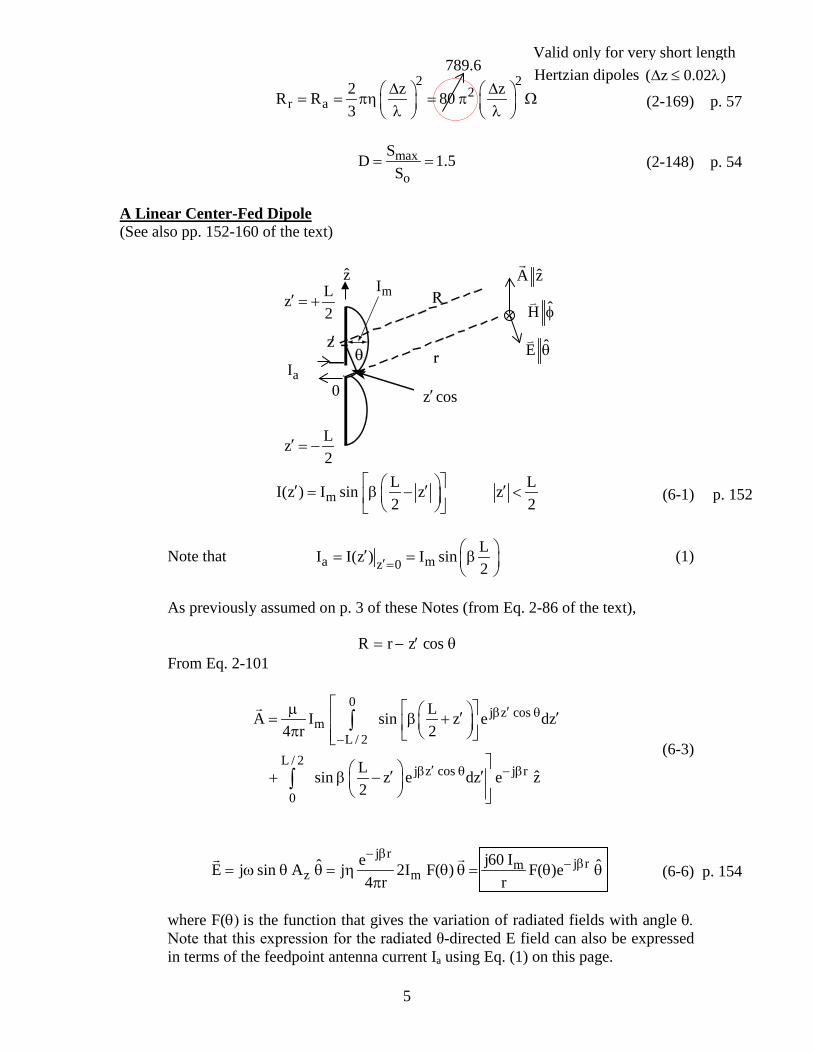
2 z zR R 803

∆ ∆ = = πη = π Ω λ λ (2-169) p. 57

max

o

SD 1.5S

= = (2-148) p. 54

A Linear Center-Fed Dipole (See also pp. 152-160 of the text)

mL LI(z ) I sin z z2 2

′ ′ ′= β − < (6-1)

Note that a mz 0LI I(z ) I sin2′=

′= = β

(1)

As previously assumed on p. 3 of these Notes (from Eq. 2-86 of the text), R = r − ′ z cos θ From Eq. 2-101

0j z cos

mL / 2

L / 2j z cos j r

0

LA I sin z e dz4 r 2

L ˆsin z e dz e z2

′β θ

−

′β θ − β

µ ′ ′= β + π ′ ′+ β −

∫

∫

(6-3)

j r

j rmz m

j60 Ieˆ ˆE j sin A j 2I F( ) F( )e4 r r

− β− β= ω θ θ = η θ θ = θ θ

π

(6-6) p. 154

where F(θ) is the function that gives the variation of radiated fields with angle θ.

Note that this expression for the radiated θ-directed E field can also be expressed in terms of the feedpoint antenna current Ia using Eq. (1) on this page.

z mI

789.6 Valid only for very short length Hertzian dipoles ( z 0.02 )∆ ≤ λ

ˆA z

ˆH φ

ˆE θ

z cos′

Lz2

′ = −

aI

Lz2

′ = +

0

p. 152

6

L Lcos cos cos2 2F( )

sin

β β θ − θ =

θ (2)

See p. 154 of the text, Fig. 6-4, for plots of F(θ) for several values of L/λ. F(θ) is always zero for angle 0θ = i.e. no radiated fields along the length of the

dipole.

( )* 2

* 2m2

2 22a rad

2 22 2a

E E 15 I1 ˆ ˆS Re E H r F ( ) r2 2 r

I P15 30 F ( )ˆF ( )rL LRr rsin sin2 2

θ θθ φ= = = θ

η π

θ= θ = ⋅

π πβ β

(3)

22

2 2mrad 2

0 0

15 IRadiated Power P S ds F ( )r sin d dr

π π= ⋅ = θ θ θ φ

π∫∫ ∫ ∫

2 2m rm a a

1 1I R I R2 2

= = (4)

2

2ma 2

a 0

60 IR F ( ) sin dI

π= θ θ θ∫ (5)

Where Ra is the antenna equivalent resistance at the feed point ( z 0′ = ). The antenna equivalent resistance Ra is given by Table l on p. 7. Thus the directivity D of a linear center-fed antenna of end-to-end length L is

given by:

2

maxmax2o a

F ( )S 120DLS R sin2

θ= =

β

(6)

7

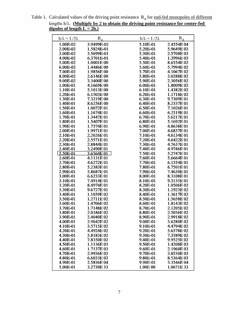
Calculated values of the driving point resistance aR for end fed monopoles of different h/λ. (Multiply by 2 to obtain the driving point resistance for dipoles.)

Table 1. Calculated values of the driving point resistance aR for end-fed monopoles of different lengths h/λ. (Multiply by 2 to obtain the driving point resistance for center-fed dipoles of length L = 2h.)

aR aR h/λ = L/2λ h/λ = L/2λ

8

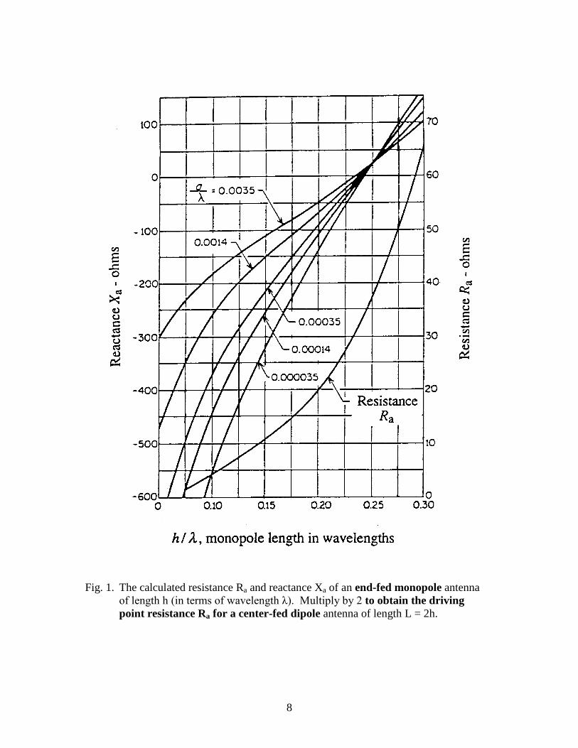
Fig. 1. The calculated resistance Ra and reactance Xa of an end-fed monopole antenna of length h (in terms of wavelength λ). Multiply by 2 to obtain the driving point resistance Ra for a center-fed dipole antenna of length L = 2h.

9

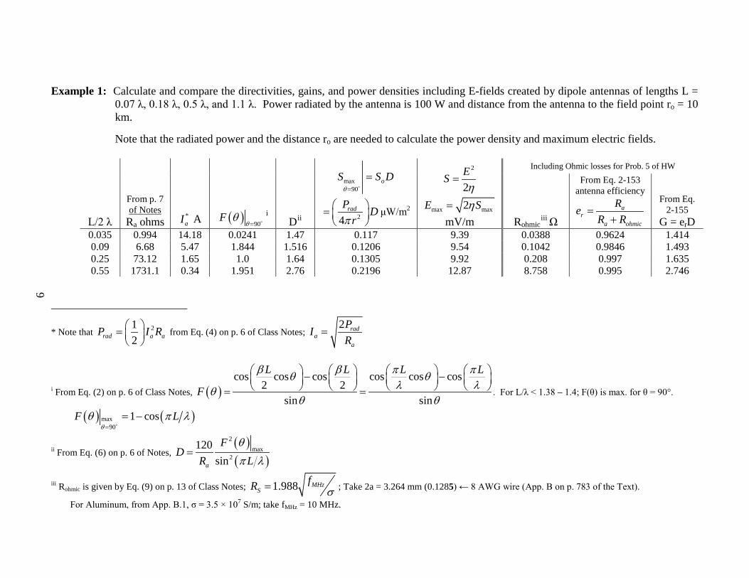
Example 1: Calculate and compare the directivities, gains, and power densities including E-fields created by dipole antennas of lengths L = 0.07 λ, 0.18 λ, 0.5 λ, and 1.1 λ. Power radiated by the antenna is 100 W and distance from the antenna to the field point ro = 10 km.

Note that the radiated power and the distance ro are needed to calculate the power density and maximum electric fields.

L/2 λ

From p. 7 of Notes

Ra ohms *aI A ( )

90F

θθ

=

i Dii

max90

oS S Dθ =

=

24radP Drπ

=

μW/m2

2

2ESη

=

max max2E Sη= mV/m

Including Ohmic losses for Prob. 5 of HW

Rohmiciii

Ω

From Eq. 2-153 antenna efficiency

ar

a ohmic

ReR R

=+

From Eq.

2-155 G = erD

0.035 0.994 14.18 0.0241 1.47 0.117 9.39 0.0388 0.9624 1.414 0.09 6.68 5.47 1.844 1.516 0.1206 9.54 0.1042 0.9846 1.493 0.25 73.12 1.65 1.0 1.64 0.1305 9.92 0.208 0.997 1.635 0.55 1731.1 0.34 1.951 2.76 0.2196 12.87 8.758 0.995 2.746

* Note that 212rad a aP I R =

from Eq. (4) on p. 6 of Class Notes;

2 rada

a

PIR

=

i From Eq. (2) on p. 6 of Class Notes, ( )cos cos cos cos cos cos

2 2sin sin

L L L L

F

β β π πθ θλ λθ

θ θ

− − = = . For L/λ < 1.38 – 1.4; F(θ) is max. for θ = 90°.

( ) ( )max90

1 cosF Lθ

θ π λ=

= −

ii From Eq. (6) on p. 6 of Notes, ( )( )

2max

2

120sina

FD

R Lθ

π λ=

iii Rohmic is given by Eq. (9) on p. 13 of Class Notes; 1.988 MHzS

fR σ= ; Take 2a = 3.264 mm (0.1285) ← 8 AWG wire (App. B on p. 783 of the Text).

For Aluminum, from App. B.1, σ = 3.5 × 107 S/m; take fMHz = 10 MHz.

9

10

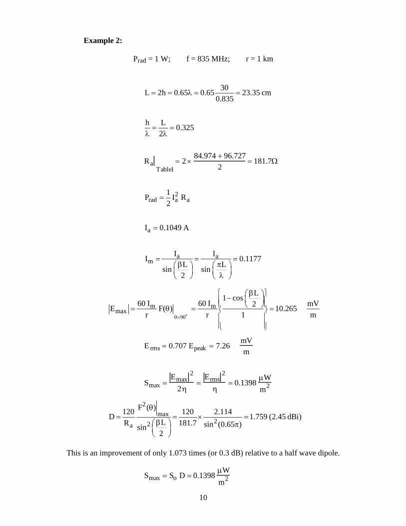
Example 2: Prad = 1 W; f = 835 MHz; r = 1 km

30L 2h 0.65 0.65 23.35 cm

0.835= = λ = =

h L 0.325

2= =

λ λ

RaTable1

= 2 ×84.974 + 96.727

2= 181.7Ω

2rad a a

1P I R2

=

aI 0.1049 A=

a am

I II 0.1177L Lsin sin2

= = =β π

λ

90

m mmax

L1 cos60 I 60 I mV2E F( ) 10.265

r r 1 mθ=

β − = θ = =

E rms = 0.707 Epeak = 7.26mVm

Smax =Emax

2

2η=

Erms2

η= 0.1398

µWm2

2max

22a

F ( )120 120 2.114D 1.759 (2.45 dBi)LR 181.7 sin (0.65 )sin2

θ= = × =

β π

This is an improvement of only 1.073 times (or 0.3 dB) relative to a half wave dipole.

Smax = So D = 0.1398µWm2

11

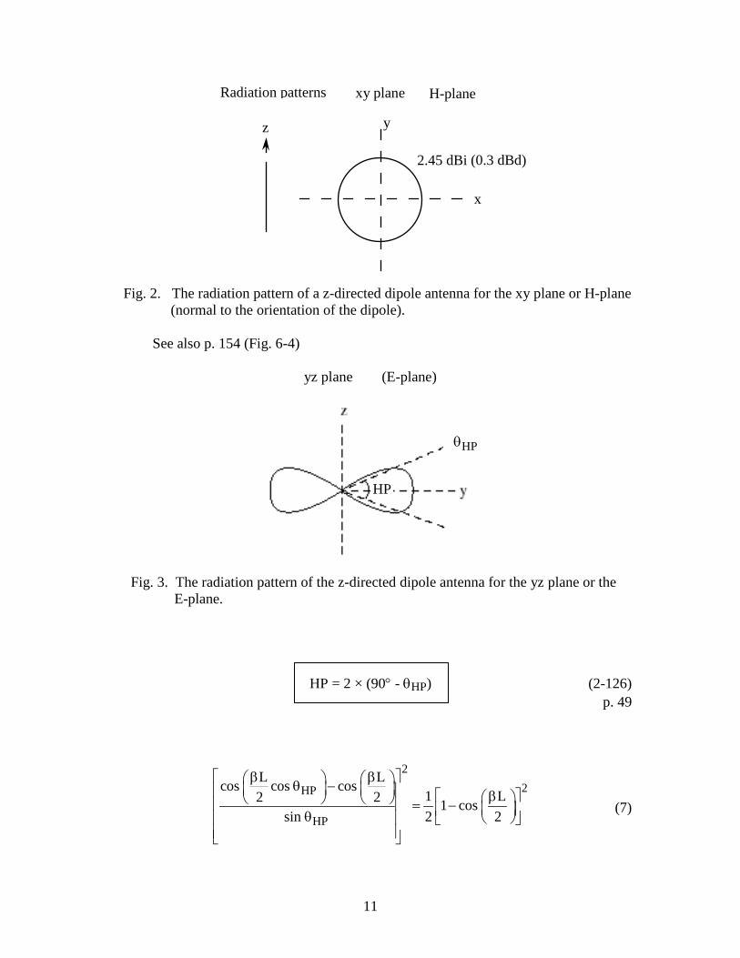
y

x

2.45 dBi

z

Fig. 2. The radiation pattern of a z-directed dipole antenna for the xy plane or H-plane (normal to the orientation of the dipole). See also p. 154 (Fig. 6-4) yz plane (E-plane)

Fig. 3. The radiation pattern of the z-directed dipole antenna for the yz plane or the E-plane. HP = 2 × (90° - θHP) (2-126) p. 49

22HP

HP

L Lcos cos cos1 L2 2 1 cos

sin 2 2

β β θ − β = − θ

(7)

HP

HPθ

Radiation patterns xy plane H-plane

(0.3 dBd)

12

pp. 57, 58 Text Ohmic Losses for a Linear Dipole

From Eq. 6-1, p. 152 Text

I( ′ z ) = Im sin β L

2− ′ z

0 ≤ ′ z ≤ L

2

= Im sin βL2

+ ′ z

−

L2

≤ ′ z ≤ 0 (1)

z 0a m

LI I(z ) I sin2′=

β ′= =

(2)

Ohmic power lost in the antenna

( )2ohmic

L/2

L/2

1P I dR2 −

= ∫ (3)

dR =d ′ z

(2πa δ)σ=

Rs d ′ z 2πa

(4)

where

s1R

2ωµ

= =σδ σ

(5)

(2-171) p. 58 is the surface resistance which depends on the conductivity σ of the material and

frequency ω (= 2πf). See App. B.1 of the Text for σ of various metals.

dR

13

L / 2 0

2 2 2 2sohmic m m

0 L / 2

R L LP I sin z dz I sin z dz4 a 2 2−

′ ′ ′ ′= β − + β + π ∫ ∫ (6)

L / 2L / 2L / 2

2 2

00 0

L 1 1 sin (2 )sin z dz sin d2 2 2

ββ ζ ′ ′β + = ζ ζ = ζ − β β ∫ ∫

1 L sin ( L)2 2 2

β β = − β (7)

where ζ = L z2

′= β +

2 2sohmic m A ohmic

R L sin ( L) 1P I 1 I R8 a ( L) 2

β= − = π β

(8)

sohmic

2

R L 1 sin ( L)R 1L4 a ( L)sin2

β= − βπ β

(9)

rad ar

in rad ohmic a ohmic

P RPeP P P R R

= = =+ +

Antenna efficiency (2-177)

Gain G = re D (2-155) For a Short Dipole (L = Δz << λ)

2

2a

zR 20 ∆ = π λ (2-172)

6 6s s

ohmicR z R LR

aπ π∆

= = (2-175)

For the general case of a linear dipole or a monopole Rohmic is calculated from the

general Eq. 9 given above. Example 3: For a Short Dipole

2 2

2a

L LR 20 197.4 = π ≅ λ λ (2-172)

See e.g. Table 1 on page 7 for L/λ =0.02, Ra = 2 × 0.0394 = 0.0788 Ω.

14

Using the conductivity of steel (see App. B.1 of the Text) σ = 2 × 106 S/m. From Eq. 2-171 or Eq. 5

3s MHzR 1.4 10 f−= × Ω

From Eq. 9, βL is small and we can expand sin x for small x

3

s sohmic 2

( L)LR L R L1 6R 1 Short dipole4 a L 6 aL

2

ββ −

= − =π β π β

(2-175)

p. 59 For L/λ = 0.02 dipole at f = 1 MHz; taking 2a = l/8" λ = 300m ; L = 6m

Rohmic =1.4 ×10−3 × 6

6π × 116

× 2.54 ×10−2= 0.2807Ω

Antenna Efficiency ar

a ohmic

R 0.0788e 0.219 (21.9%)R R 0.0788 0.2807

= = =+ +

Gain G = re D = 0.219 ×1.5 = 0.3285. Note that for short dipoles of thin wires, the ohmic resistance can be substantial

and even larger than Ra. Therefore, this leads to reduced efficiency of radiation. Example 4: For a Half Wave Dipole

L = 0.5λ; Ra = 73.12 Ω; βL2

=πLλ

=π2

; βL = π; f = 10 MHz; L = 15m; 2a = 1/8"

From Eq. 9

( )3

sohmic

2

1.4 10 10 15R LR 3.3314 a 4 2.54 10

16

−

−

× ×= = = Ω

π π× × ×

r73.12e 0.9565 (95.65%)

73.12 3.33= =

+

G = 0.9565 D = 0.9565 × 1.64 = 1.568

15

pp. 75-81 Text Dipoles Versus Monopoles Above a Perfect Ground or Reflector

For 0 180≤ θ ≤ For 0 90≤ θ ≤

( )60 ˆj rmIE j F er

βθ θ−=

(2) ( )60 ˆj rmj IE F er

βθ θ−′′ =

(3)

( )2

22

15 ˆmIS F rr

θπ

=

(4) ( ) ( )2 2

2 22 2

2

15 15ˆ ˆsin

2

m aI IS F r F rLr r

θ θβπ π

′ ′′ = =

(5)

212rad a aP I R= (6) 21

2rad a aP I R′ ′ ′= (7)

F( )θ is given as Eq. (2) on p. 6 of the Notes. Since a monopole radiates in the upper half space while a dipole radiates both in

the upper and lower half spaces,

12dipole monopoleS S ′= for identical radiated powers (8)

2monopole dipoleD D′ = (9)

12

a a

a amonopole dipole

R RX X

′=

′ (10)

For identical radiated powers

2a aI I′ = (11)

2m mI I′ = (12)

Image antenna

aI aI′

I(z′) same as on page 5 of the Notes ( ) sin 02 2mL LI z I z zβ ′ ′ ′ ′= − ≤ ≤

(1)

16

Example 4: h

λ=

L2λ

= 0.35 Monopole Antenna

f = 1.5 MHz, λ = 200 m ; r = 1 km h =

L2

= 70 m ; Prad = 103 W (1 KW)

From Table 1 on page 7, ′ R a =127.1 Ω (do not multiply by 2 for monopoles) From Eq. 7, aI 3.967A′ = From Eq. 5,

monopole

2

22

6 2

90

L Lcos cos cos15 (3.967) 2 2S 0.29 mW / m

sin10 sin (0.7 )θ=

β β θ − ′ = × =

θπ× π

monopole dipolerado 2

SD 3.64 2 DPS4 r

′′ = = = ×

=π

From Eq. (6) on p. 6 of Class Notes

2max

2a

F ( )120DLR sin2

θ=

β

Note that L h2

= which is the height of the monopole.

17

pp. 84-89 Small Diameter (<< λ) Loop Antennas The loop antenna is a radiating (or receiving) coil of one or more turns of circular

or rectangular form. Ferrite or air core loops are used extensively in radio receivers, direction finders, aircraft receivers, and UHF transmitters.

The theory of loop antennas is derived in a manner similar to the General Theory

of Conduction Current Antennas given on page 44 of Text and on page 2 of my handout notes.

We start by assuming, as seen in Fig. 1, that the current I in the loop has the same

magnitude and phase. This is certainly possible for small diameter loops where 2πb < λ/10.

Fig. 1. A circular loop antenna of radius 'b'. From General Theory of Conduction Current Antennas, from Eq. 2-101,

A =

µ4π

I ˆ ′ φ e− jβR

R0

2π∫ bd ′ φ (1)

( ) ( )2 2 2R x x y y z′ ′= − + − + (2) ′ x = b cos ′ φ ; ′ y = b sin ′ φ ; ′ z = 0; x = r sin θ; y = 0; z = r cos θ (3) Note that we have defined the x-axis (the choice of which is arbitrary) such that

the field point lies in the xz plane. The field point F, therefore, has coordinates (x, 0, z) in Cartesian coordinate system and (r, θ, 0) is spherical coordinate system.

Substituting Eq. 3 into Eq. 2

1/ 22 2 bR r b 2 br sin cos r 1 sin cosr

r bsin cos

′ ′= + − θ φ ≅ − θ φ ′= − θ φ (4)

R

x

r

z

Loop in the xy plane

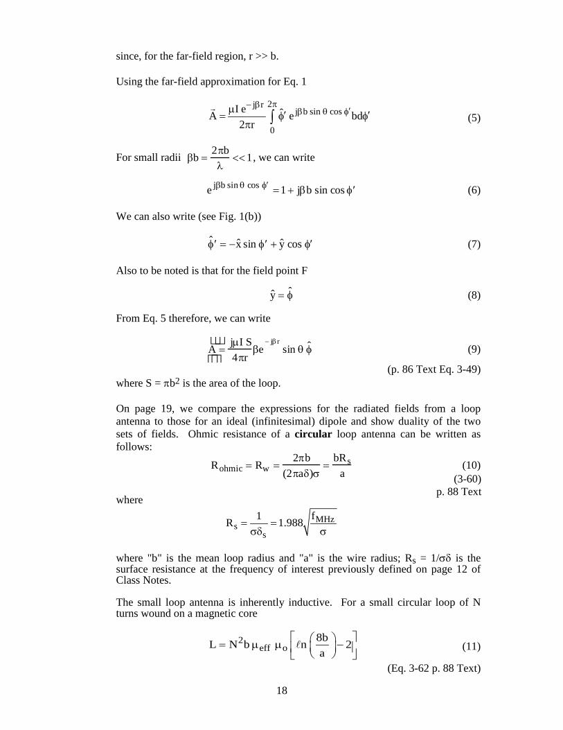
18

(3-60) p. 88 Text

since, for the far-field region, r >> b. Using the far-field approximation for Eq. 1

2j r

j b sin cos

0

I e ˆA e bd2 r

π− β′β θ φµ ′ ′= φ φ

π ∫

(5)

For small radii βb =2πbλ

<<1, we can write

e jβb sin θ cos ′ φ =1 + jβb sin cos ′ φ (6) We can also write (see Fig. 1(b)) ˆ ′ φ = − ˆ x sin ′ φ + ˆ y cos ′ φ (7) Also to be noted is that for the field point F

ˆ y = ˆ φ (8) From Eq. 5 therefore, we can write

A =

jµI S4πr

βe− jβr

sin θ ˆ φ (9)

(p. 86 Text Eq. 3-49) where S = πb2 is the area of the loop. On page 19, we compare the expressions for the radiated fields from a loop

antenna to those for an ideal (infinitesimal) dipole and show duality of the two sets of fields. Ohmic resistance of a circular loop antenna can be written as follows:

Rohmic = Rw =2πb

(2πaδ)σ=

bRsa

(10)

where

MHzs

s

f1R 1.988= =σδ σ

where "b" is the mean loop radius and "a" is the wire radius; Rs = 1/σδ is the

surface resistance at the frequency of interest previously defined on page 12 of Class Notes.

The small loop antenna is inherently inductive. For a small circular loop of N

turns wound on a magnetic core

2eff o

8bL N b n 2a

= µ µ − (11)

(Eq. 3-62 p. 88 Text)

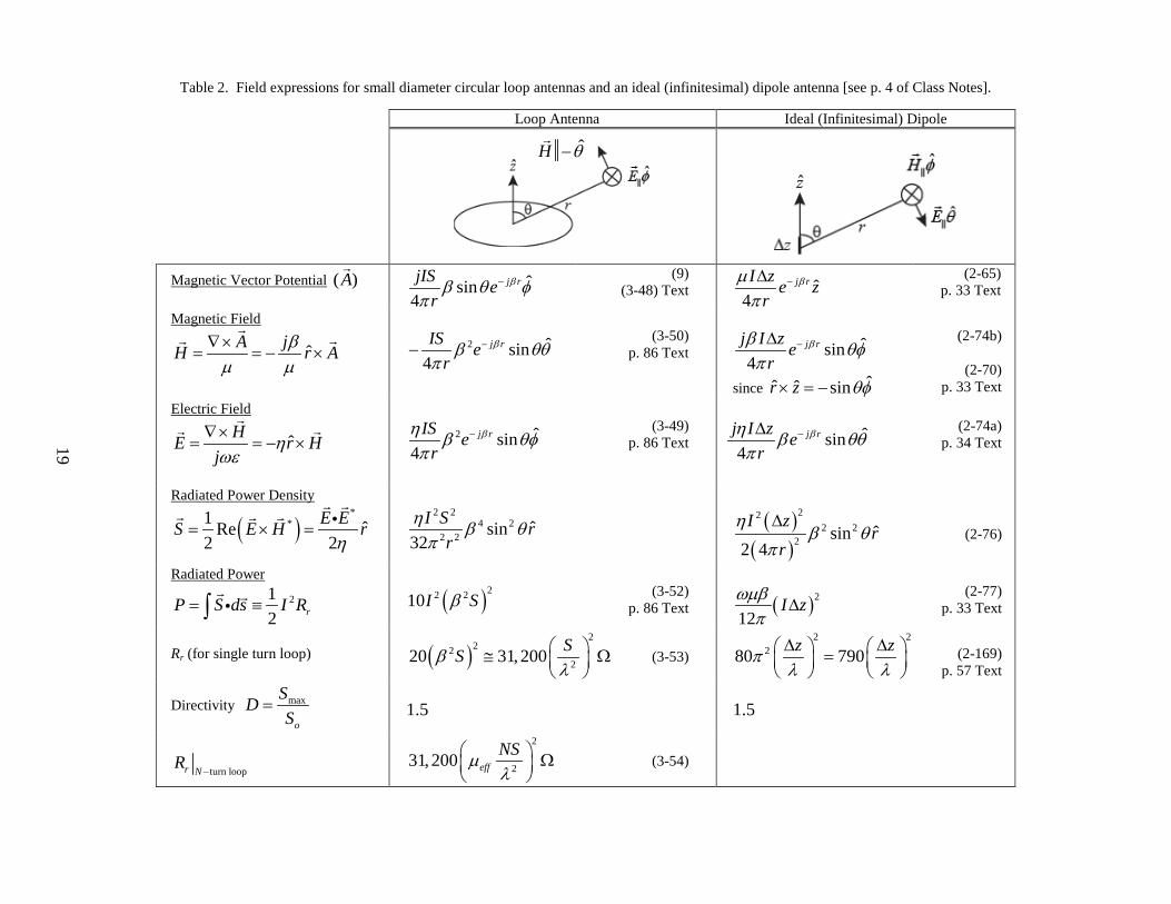
19

Table 2. Field expressions for small diameter circular loop antennas and an ideal (infinitesimal) dipole antenna [see p. 4 of Class Notes].

Loop Antenna Ideal (Infinitesimal) Dipole

Magnetic Vector Potential ( )A

ˆsin4

j rjIS er

ββ θ φπ

− (9) (3-48) Text ˆ

4j rI z e z

rβµ

π−∆

(2-65) p. 33 Text

Magnetic Field

ˆA jH r Aβµ µ

∇×= = − ×

2 ˆsin

4j rIS e

rββ θθ

π−−

(3-50) p. 86 Text

ˆsin4

j rj I z er

ββ θφπ

−∆

since ˆˆ ˆ sinr z θφ× = −

(2-74b) (2-70) p. 33 Text

Electric Field

ˆHE r Hj

ηωε

∇×= = − ×

2 ˆsin

4j rIS e

rβη β θφ

π−

(3-49) p. 86 Text

ˆsin4

j rj I z er

βη β θθπ

−∆

(2-74a) p. 34 Text

Radiated Power Density

( )*

*1 ˆRe2 2

E ES E H rη

= × =

2 2

4 22 2

ˆsin32

I S rr

η β θπ

( )( )

222 2

2 ˆsin2 4I z

rr

ηβ θ

π

∆ (2-76)

Radiated Power 21

2 rP S ds I R= ≡∫

( )22 210I Sβ

(3-52) p. 86 Text

( )2

12I zωµβ

π∆

(2-77) p. 33 Text

Rr (for single turn loop) ( )

222

220 31,200 SSβλ

≅ Ω

(3-53) 2 2

280 790z zπλ λ∆ ∆ =

(2-169) p. 57 Text

Directivity max

o

SDS

= 1.5

1.5

turn loopr NR

−

2

231,200 effNSµλ

Ω

(3-54)

ˆH θ−

19

20

For an N-turn loop, Rohmic is also higher proportional to overall length of the wire Rohmic

N− turnloop

= NbRs

a (12)

The effective permeability μeff depends not only on the permeability μr of the

ferrite core material, but also on the core geometry, i.e., length to diameter ratio R, given as follows:

( )1 1

reff

rDµµµ

=+ −

(13)

where 4D is the demagnetization factor approximately given by D [4] 1.440.37D R−

(14) p. 87 Text Example 5 (see also Ex. 3-1, p. 88, Text): Calculate the input impedance, directivity, and gain for an N = 1000 turn loop

antenna wound with a AWG 22 copper wire on a ferrite rod of diameter 3/4". This antenna is to be used at a frequency of 1.5 MHz. It is given that µeff = 50 for the ferrite that is used.

Solution: From p. 783 of the Text, for AWG 22 wire d = 2a = 0.644 mm ⇒

0.025 ′ ′ 3 From p. 58, Eq. 2-171

MHzs

f1R 1.988 ohms2ωµ

= = =σδ σ σ

(15)

For copper σ = 5.7 × 107 S/m (p. 783, Text); Rs = 3.22 ×10-4 Ω at f = 1.5 MHz

Mean loop radius b =′ ′ 3 8

+ a = 9.847 mm

From Eq. 12, for N = 1000-turn loop Rohmic = 9.85Ω From Eq. 3-54 Text (see also p. 19 of Class Notes)

𝑅𝑟 = 31,200 𝜇𝑒𝑓𝑓 𝑁𝑆𝜆22

= 45Ω (3-54) Text 4 R. Pettengill, H. Garland, and J. Mendl, “Receiving antennas for miniature receivers,” IEEE Transactions on Antennas and Propagation, Vol AP-26, pp. 528-530, July 1977.

21

From Eq. 11 above

6L 0.232H L 2 1.5 10 0.232 2.18 M= ⇒ ω = π× × × = Ω D = 1.5; 𝑒𝑟 = 𝑅𝑟

𝑅𝑜ℎ𝑚𝑖𝑐+𝑅𝑟= 0.82 (82%)

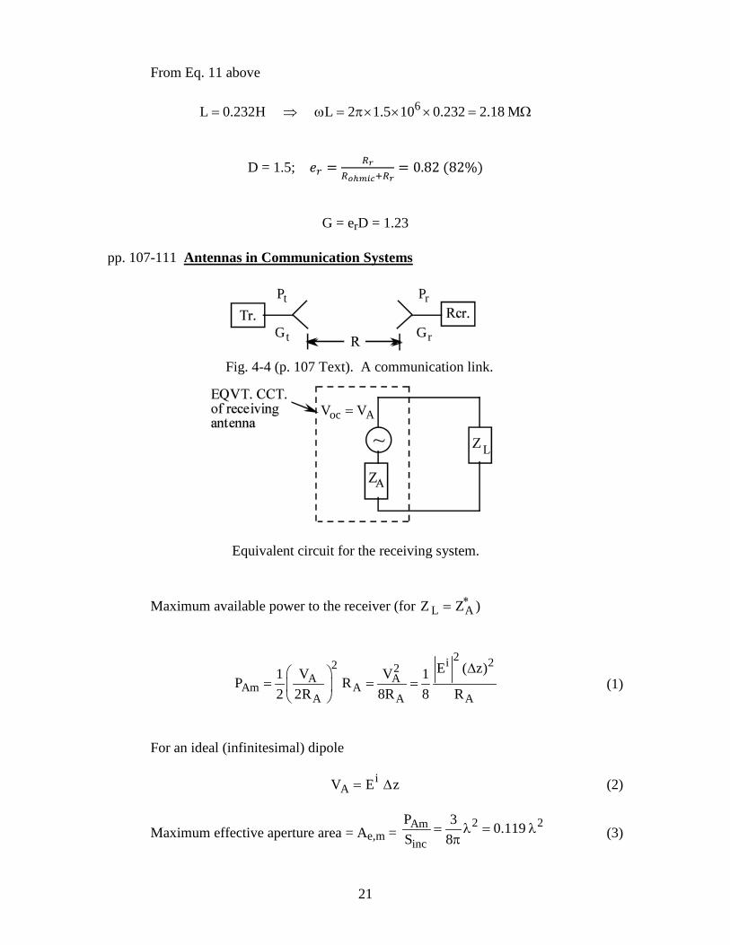
G = erD = 1.23 pp. 107-111 Antennas in Communication Systems

Maximum available power to the receiver (for Z L = ZA

∗ )

2i 22 2A A

Am AA A A

E ( z)V V1 1P R2 2R 8R 8 R

∆ = = =

(1)

For an ideal (infinitesimal) dipole VA = Ei ∆z (2)

Maximum effective aperture area = Ae,m = 2 2Am

inc

P 3 0.119S 8

= λ = λπ (3)

oc AV V=

tP rP

rG tG

Fig. 4-4 (p. 107 Text). A communication link.

Equivalent circuit for the receiving system.

22

2i

incS E 2= η (4) D = 1.5 for an ideal dipole (5) (4-22)

2e,m2 2

4 4 3D A 1.58

π π= = × λ =

πλ λ (6)

(4-23) Text For a general antenna, therefore

G =4πλ2 Ae

(7)

Ae = er Aem effective aperture area of an antenna (4-27) p. 108 Text Available power including also the antenna losses PA = S Ae (4-26) Text

S = GtPt

4πR2 (4-31)

2

t t t rr er er t2 2

G P G GP SA A P4 R (4 R)

λ = = =

π π (4-33)

or

et err t 2 2

A AP PR

=λ

Friis transmission formula (4-33)

We can also write Eq. (4-33) in dB-form as follows:

r t t rP (dBm) P (dBm) G (dB) G (dB) 20log R(km)20log f (MHz) 32.44

= + + −

− − (4-34)

Example 6: For Ground Based TV Stations Say, Channel 5 f = 76 - 82 MHz f ≅ 80 MHz λ = 3.75 m Prad ~ 5 - 10 kW say, 10 kW = 104 W (40 dBW)

23

Gt ~ 20 - 50 (factor) say, tG = 30 (factor) ⇒ (14.77 dB ~ 15 dB) EIRP = Gt Prad → 55 dBW → 5.510 W (85 dBm) Rmax ~ 20 - 30 miles ~ 50 km; since 1 mile = 1.6 km say Gr ≅ 7 dB ≅ 5

Ae,r =λ2

4πGr = 5.6 m2

Using the logarithmic form of the Friis communication link formula Eq. (4-34)

r12.5

P (dBm) 70 15 7 34.0 38.06 32.44

12.5 dBm 10 mW 56.2 W−

= + + − − −

= − = = µ

Example 7: Calculate the open-circuit voltage developed across an antenna of resistance RA=

80 ohms for the above-calculated incident power density

rinc 2e

P 56.2 WS 10A 5.6 m

µ= = =

Assume RA= 80Ω

2 2oc A

inc eA A

V V power picked up and delivered to a matched load S A8R 8R

→ = =

6

oc A inc e,r rV 8R S A 8 80 P 640 56.2 10

188.65 mV 0.19V

−= = × = × ×

=

24

Chapter 8 -- Antenna Arrays (see pp. 271..... Text)

For a uniformly excited (UE), equally-spaced linear array (ESLA)

For N identical radiating elements (length, orientation, etc.) that are excited with

identical magnitudes but progressively phase-shifted currents i.e. 2 ( 1), , ,j j j NI I e I e I eα α α− − − −

(1) we can write the total electric field

E T as follows

N 11 j rj rj rT o 1 N 1E E e E e E e −− β⋅β⋅− β⋅

−= + +

(1)

r = xˆ x + yˆ y + zˆ z r 1 = (x − d)ˆ x + yˆ y + zˆ z

(2)

[ ]ˆ ˆ ˆsin cos x sin sin y cos zβ = β θ φ + θ φ + θ

(3) From Eq. 1, we can write

j r j j d sin cos 2 j 2 j d sin cosT o

N 1j r jn

on 0

E E e 1 e e e e

E e e

− β⋅ − α β θ φ − α β θ φ

−− β⋅ ψ

=

= + + +

= ∑

(4)

(3-16)

since

( ) ( )1 2r r d sin cos ; r r 2 d sin cosβ⋅ − = −β θ φ β⋅ − = − β θ φ

(6)

d cos φ

F(x,y,z)

25

From Eq. 4

E T =

E o ⋅ AF

where

N 1 jN

jnj

n 0

1 eArray Factor AF e1 e

− ψψ

ψ=

−= =

−∑ (7)

AF = ej(N−1)ψ / 2 sin(Nψ / 2)sin(ψ / 2)

(8)

(8-19) p. 279 Text

Normalized AF f(ψ) =sin(N ψ / 2)N sin(ψ / 2)

(9)

(8-22 Text) UE, ESLA where

( )( )

x x

y y

ˆd sin cos for an x directed array

ˆd sin sin for a y directed array

ψ = β θ φ − α −

= β θ φ − α −

( )z z ˆd cos for a z directed array= β θ − α − (see Eq. 3-19 Text) (10)

E T = N

E o f(ψ) =

E o

sin(N ψ / 2)sin(ψ / 2)

(11)

H T =

∇ ×E T

jωµo= −

jβjωµo

ˆ r ×E T (12)

( )*

* T TT T

E E1 ˆS Re E H r2 2

⋅= × =

η

(13)

* From Eq. 11, for directions of max radiation 0, , 2 ,2ψ

= ± π ± π

p. 280 Text A number of trends can be seen by examining the normalized array factor |f(ψ)|. 1. As N increases the main lobe narrows. Peak for the main lobe occurs for

ψ = 0 where |f(ψ)| =1.

*

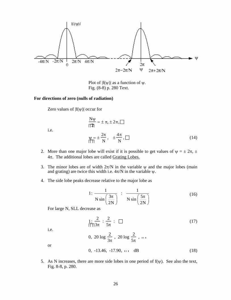
26

Plot of |f(ψ)| as a function of ψ. Fig. (8-8) p. 280 Text. For directions of zero (nulls of radiation) Zero values of |f(ψ)| occur for

Nψ2

= ± π, ± 2π,

i.e.

ψ = ±

2πN

, ±4πN

, (14)

2. More than one major lobe will exist if it is possible to get values of ψ = ± 2π, ±

4π. The additional lobes are called Grating Lobes. 3. The minor lobes are of width 2π/N in the variable ψ and the major lobes (main

and grating) are twice this width i.e. 4π/N in the variable ψ. 4. The side lobe peaks decrease relative to the major lobe as

1 11: :

3 5N sin N sin2N 2N

π π

(16)

For large N, SLL decrease as

1:

23π

:2

5π: (17)

i.e. 0, 20 log 2

3π , 20 log 2

5π ,

or 0, -13.46, -17.90, dB (18) 5. As N increases, there are more side lobes in one period of f(ψ). See also the text,

Fig. 8-8, p. 280.

27

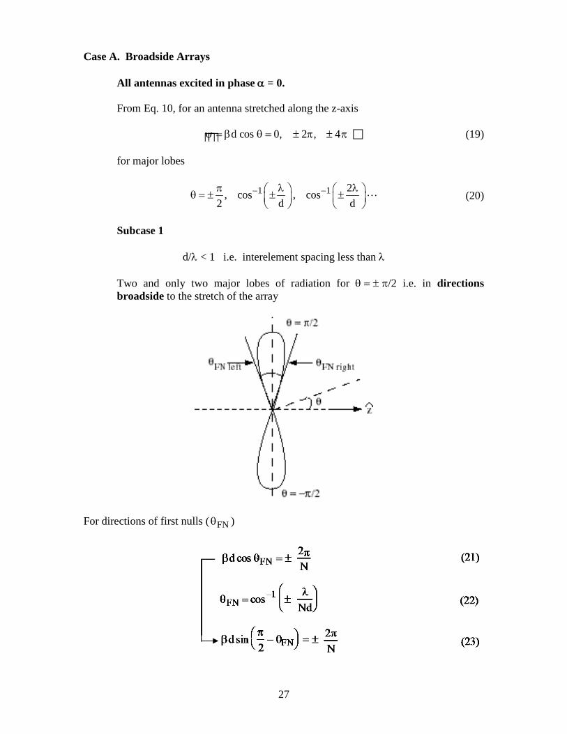
Case A. Broadside Arrays All antennas excited in phase α = 0. From Eq. 10, for an antenna stretched along the z-axis ψ = βd cos θ = 0, ± 2π, ± 4π (19) for major lobes

1 1 2, cos , cos2 d d

− −π λ λ θ = ± ± ±

(20)

Subcase 1 d/λ < 1 i.e. interelement spacing less than λ Two and only two major lobes of radiation for θ = ± π/2 i.e. in directions

broadside to the stretch of the array

For directions of first nulls ( FNθ )

28

FN left FN rightBWFN θ θ= − (24)

1 1cos cosNd Ndλ λ− − = − −

(25)

(8-31) p. 283 Text

1 22sin 114.6radiansNd Nd Ndλ λ λ− = ≅ = °

(26)

(8-33) for Nd >> λ

Example 6:

d/λ = 0.5 , N = 8 From Eq. 23

1FN

1sin 14.52 4

−π − θ = ± = ±

(27)

BWFN = 29° (28) Angle for first-side lobe

Nsin 12ψ = ±

from Eq. 11 Nψ

2= 4 βd cos θ( ) =

8πdλ

cos θ = ±3π2

(29)

1 3cos 68 ; 1128

− θ = ± = ± ±

(30)

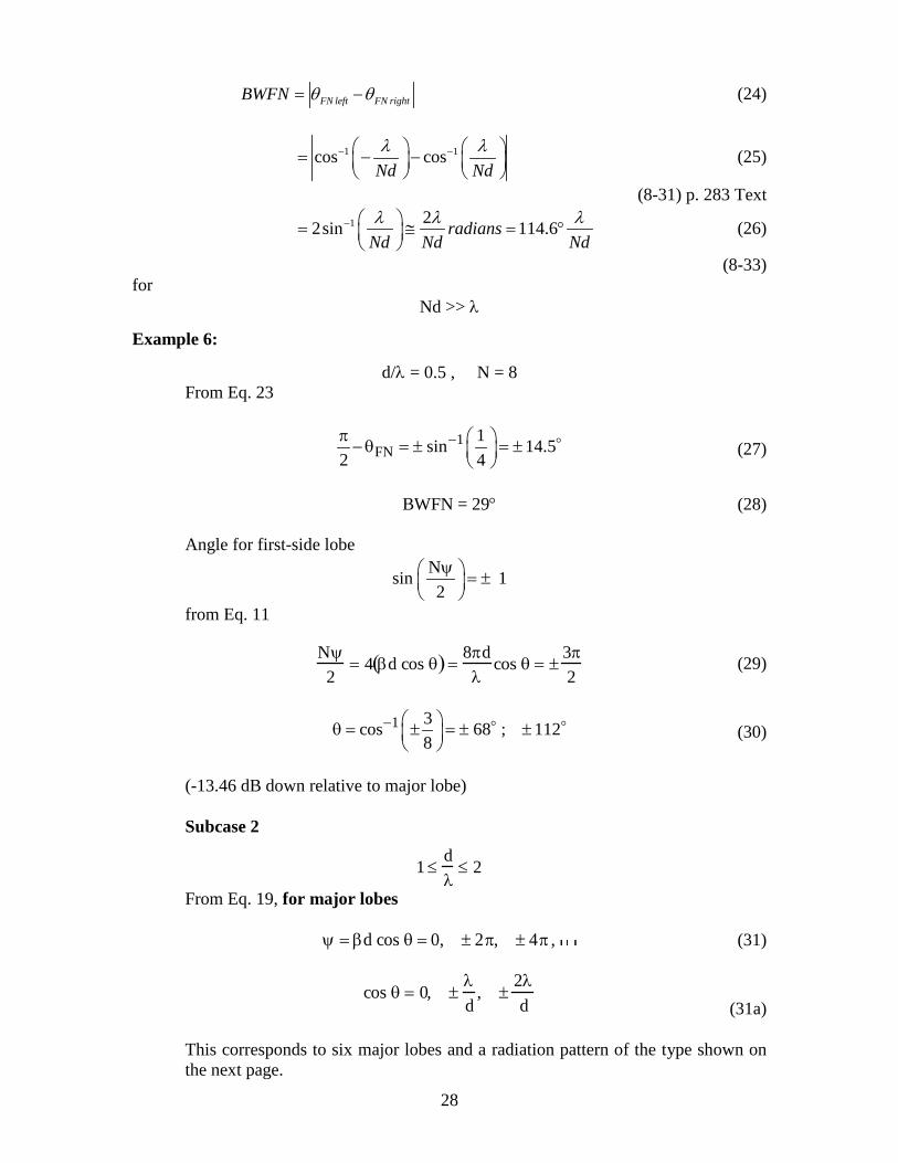
(-13.46 dB down relative to major lobe) Subcase 2

1 ≤dλ

≤ 2

From Eq. 19, for major lobes ψ = βd cos θ = 0, ± 2π, ± 4π , (31)

cos θ = 0, ±λd

, ±2λd (31a)

This corresponds to six major lobes and a radiation pattern of the type shown on

the next page.

29

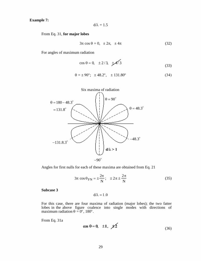
Example 7: d/λ = 1.5 From Eq. 31, for major lobes 3π cos θ = 0, ± 2π, ± 4π (32) For angles of maximum radiation

cos θ = 0, ± 2 / 3, ± 4/ 3

(33) θ = ± 90°; ± 48.2°, ± 131.80° (34)

Angles for first nulls for each of these maxima are obtained from Eq. 21 3π cos θFN = ±

2πN

; ± 2π ±2πN

(35)

Subcase 3 d/λ = 1.0 For this case, there are four maxima of radiation (major lobes); the two fatter

lobes in the above figure coalesce into single modes with directions of maximum radiation θ = 0°, 180°.

From Eq. 31a

(36)

Six maxima of radiation

48.3θ =

48.3−

90θ = 180 48.3

131.8

θ = −

=

131.8.3−

90−

d/λ > 1

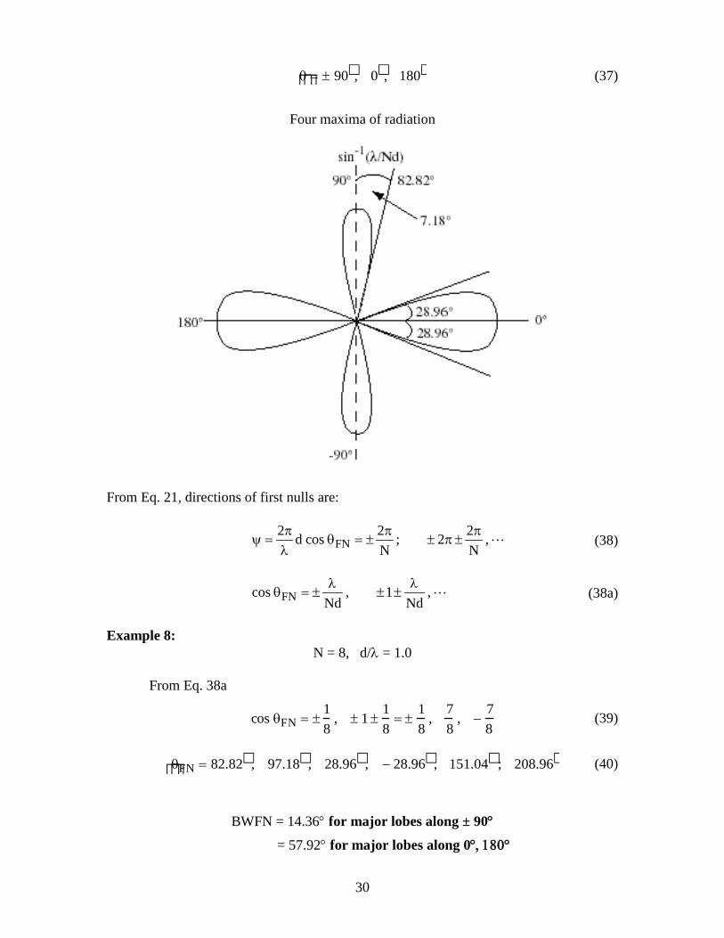
30

θ = ± 90, 0, 180 (37)

Four maxima of radiation

From Eq. 21, directions of first nulls are:

FN2 2 2d cos ; 2 ,

N Nπ π π

ψ = θ = ± ± π ±λ

(38)

FNcos , 1 ,Nd Ndλ λ

θ = ± ± ± (38a)

Example 8: N = 8, d/λ = 1.0 From Eq. 38a

cos θFN = ±18

, ± 1 ±18

= ±18

,78

, −78

(39)

θFN = 82.82, 97.18, 28.96, − 28.96, 151.04; 208.96 (40) BWFN = 14.36° for major lobes along ± 90°

= 57.92° for major lobes along 0°, 180°

31

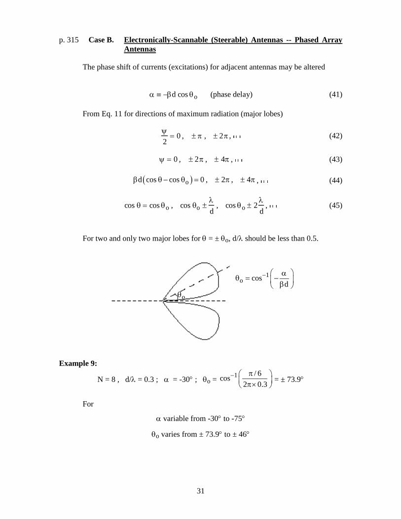
p. 315 Case B. Electronically-Scannable (Steerable) Antennas -- Phased Array Antennas

The phase shift of currents (excitations) for adjacent antennas may be altered α ≡ −βd cos θo (phase delay) (41) From Eq. 11 for directions of maximum radiation (major lobes) ψ

2= 0 , ± π , ± 2π , (42)

ψ = 0 , ± 2π , ± 4π , (43) ( )od cos cos 0 , 2 , 4β θ − θ = ± π ± π , (44)

cos θ = cos θo , cos θo ±λd

, cos θo ± 2λd

, (45)

For two and only two major lobes for θ = ± θo, d/λ should be less than 0.5.

Example 9:

N = 8 , d/λ = 0.3 ; α = -30° ; θo = 1 / 6cos2 0.3

− π π×

= ± 73.9°

For

α variable from -30° to -75°

θo varies from ± 73.9° to ± 46°

1o cos

d− α

θ = − β

oθ

32

0.4167

For directions of zero radiation, from Eq. (14) on p. 25 of Class Notes,

2

Nψ π= ±

2Nπψ = ±

( ) 2cos cos odNπβ θ θ− = ±

2cos cosFN o N dπθ θβ

= ±

1 2cos cosFN o N dπθ θβ

− = ±

1cos cos o Ndλθ− = ±

(45a)

Example 9 (continued): d/λ = 0.3 , N = 8 α = -30° = -π/6 θo = ±73.9°

1 1cos 0.27732.4FNθ − = ±

= 46.05° ; 98.01° BWFN = 51.96° Example 9, Part B: Let us compare the antenna array of N = 8, d = 0.3λ for the

following three conditions:

α Direction of

max radiation BWFN

0 Broadside array θo = ±90°

from Eq. (20) on p. 27

of Class Notes

from Eq. (26) on p. 28 of Class Notes

12sinBWFNNdλ− =

= 49.25° -30°

from Ex. 9 on this page

directions of max radiation

θo = ±73.9° θo = ±73.9° BWFN = 51.96°

-108° End fire antenna

array α = -βd

θo = 0° 12cos 1BWFN

Ndλ− = −

= 108.6° See Eq. 52 on p. 36 of Class Notes

33

For a one-dimensional antenna array The array factor of a one-dimensional antenna array from Eq. (8) of Class Notes

p. 25 is as follows:

( )sin 2sin 2

NAF

ψψ

= (1)

Where ψ is given by Eq. (1) on p. 25 of Class Notes. From Eq. (1) here, for directions of max radiation ψ = 0, ±2π, … For directions of zero radiation or nulls of radiation

, 2 ,2

Nψ π π= ± ±

or ψ = ±2π/N for first nulls of radiation. Table of general relationships for one-dimensional z-directed phased array antennas

α

directions of max. radiation principal lobe/s

ψ = 0 directions of first nulls

derived on p. 32 BWFN

0 θo = ±90° broadside array

1cos cos o Ndλθ− ±

1cosNdλ− = ±

see Eq. (22) on p. 27 of Class Notes

12sinNdλ−

see Eq. (26) on p. 28 of Class Notes

α 1coso d

αθβ

− = −

see p. 31 of Class Notes

1cos cos o Ndλθ− ±

1cosd Nd

α λβ

− = − ±

see Eq. 45a on p. 32

of Class Notes

calculate θFN1, θFN2

BWFN = θFN2 - θFN1

α = -βd θo = cos-1 (1)

= 0° End fire array

1cos 1Ndλ− −

12cos 1Ndλ− −

14sin2Nd

λ− =

see Eq. 52 on p. 36 of Class Notes

z

34

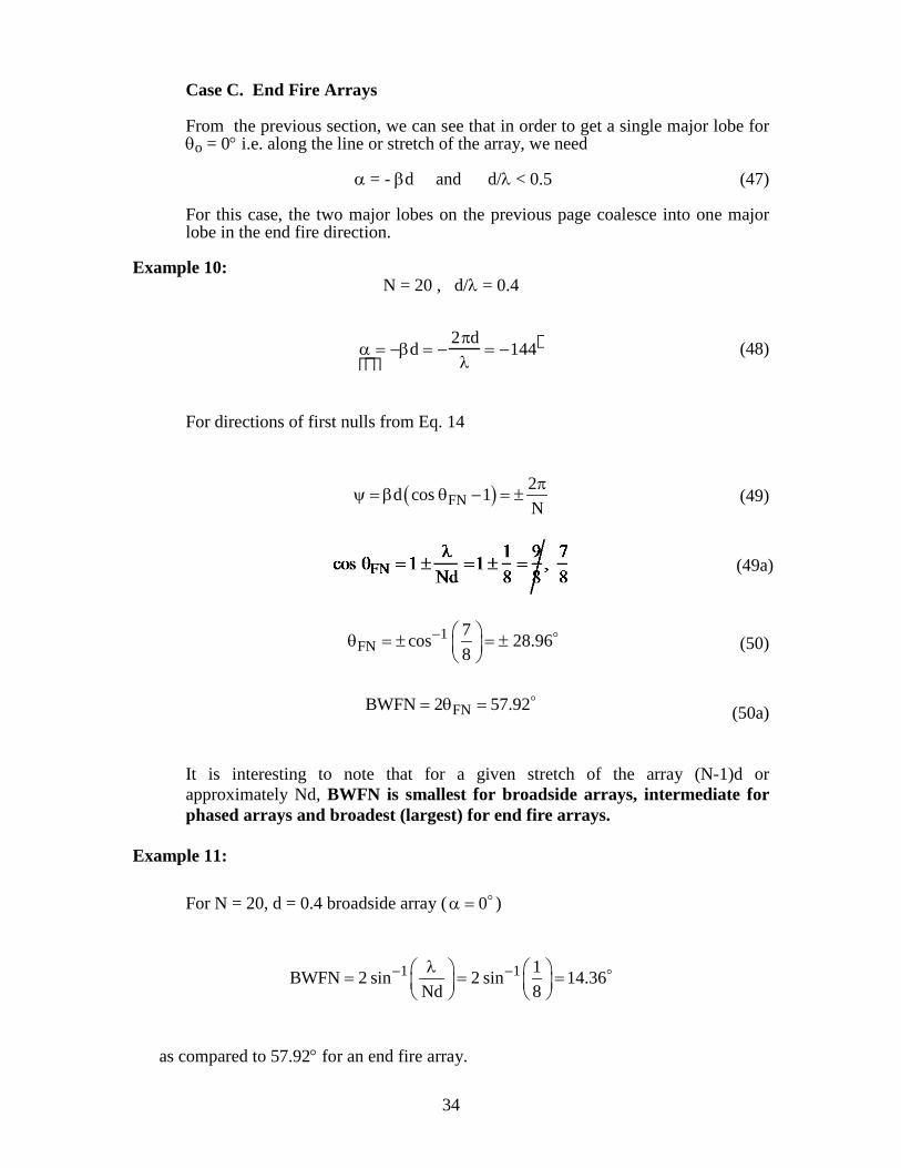
Case C. End Fire Arrays From the previous section, we can see that in order to get a single major lobe for

θo = 0° i.e. along the line or stretch of the array, we need α = - βd and d/λ < 0.5 (47) For this case, the two major lobes on the previous page coalesce into one major

lobe in the end fire direction. Example 10: N = 20 , d/λ = 0.4

α = −βd = −

2πdλ

= −144 (48)

For directions of first nulls from Eq. 14

( )FN2d cos 1Nπ

ψ = β θ − = ± (49)

1FN

7cos 28.968

− θ = ± = ±

(50)

FNBWFN 2 57.92= θ =

(50a) It is interesting to note that for a given stretch of the array (N-1)d or

approximately Nd, BWFN is smallest for broadside arrays, intermediate for phased arrays and broadest (largest) for end fire arrays.

Example 11: For N = 20, d = 0.4 broadside array ( 0α = )

1 1 1BWFN 2 sin 2 sin 14.36Nd 8

− −λ = = =

as compared to 57.92° for an end fire array.

(49a)

35

rather than 7/8 or 0.875 in Eq. 49a

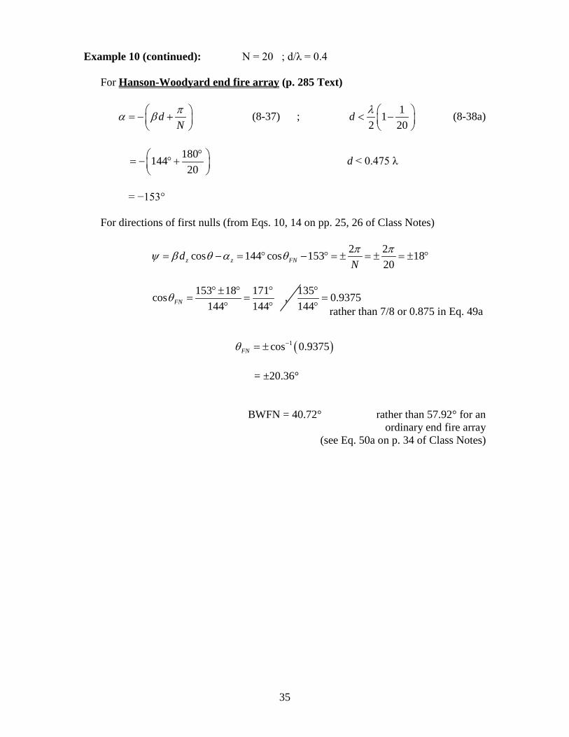
Example 10 (continued): N = 20 ; d/λ = 0.4 For Hanson-Woodyard end fire array (p. 285 Text)

dNπα β = − +

(8-37) ; 11

2 20d λ < −

(8-38a)

18014420

° = − ° +

d < 0.475 λ

= −153° For directions of first nulls (from Eqs. 10, 14 on pp. 25, 26 of Class Notes)

2 2cos 144 cos 153 1820z z FNd

Nπ πψ β θ α θ= − = ° − ° = ± = ± = ± °

153 18 171cos144 144FNθ ° ± ° °

= =° °

, 135 0.9375144

°=

°

( )1cos 0.9375FNθ −= ± = ±20.36° BWFN = 40.72° rather than 57.92° for an ordinary end fire array (see Eq. 50a on p. 34 of Class Notes)

36

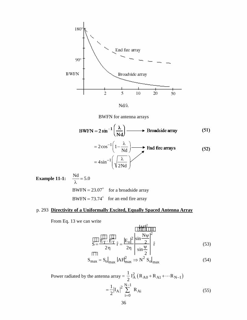
Nd/λ BWFN for antenna arrays

Nd 5.0

BWFN 23.07

BWFN 73.74

=λ

=

=

p. 293 Directivity of a Uniformally Excited, Equally Spaced Antenna Array From Eq. 13 we can write

S =

E T ⋅

E T

*

2ηˆ r =

Eo2

2η

sinNψ2

sin ψ2

2AF 2

ˆ r (53)

Smax = So max AFmax2 ⇒ N2 So max (54)

Power radiated by the antenna array = ( )2A A0 A1 N 1

1 I R R R2 −+ +

N 12

A Aii 0

1 I R2

−

== ∑ (55)

1

1

2cos 1Nd

4sin2Nd

−

−

λ = − λ

=

for a broadside array

for an end fire array

Example 11-1:

37

In general 2 A0oarray N 1

Aii 0

RD N DR

−

=

=

∑ (55a)

where oD and A0R pertain to an isolated element of the antenna array. Ignoring Mutual Impedance Effects RA0 = RA1, = RN-1 Power radiated by the antenna array = 1

2IA

2 RA0 N = N Po (56)

where Po is the power radiated by the zeroth element

2

max maxo o

o2

AFSD D D NN P N4 r

= = ⋅ =

π

(57)

where Do is the directivity of each of the antenna elements. Example 12:

Calculate the directivity of an antenna array of 20 half wavelength (L = λ/2) dipoles that are fed in phase and consequently radiate in broadside directions. Neglect the mutual impedance effects for this problem.

Solution:

2max

oAF

D ND 20 1.64 32.8N

= = = × =

Example 13: a. Calculate the directivity/gain of an array of 30 vertical monopoles above ground

each of length H = L/2 = 0.35 λ that are spaced a distance d = 0.2λ from each other.

b. Calculate the relative phase difference between monopoles if the major lobe of

radiation is to be in the end fire direction assuming an ordinary end fire array. c. Calculate the BWFN for this array. Solution: a. D = N Do = 30 × 3.636 = 109.08 b. From Eq. 47

α = −βd = −

2πdλ

= −72

38

Each of the successive elements should be fed with a current that is lagging in phase by 72° from the previous element.

c. From Eq. 49a,

cos θFN = 1 −λ

Nd=1 −

λ6λ

= 1−16

=56

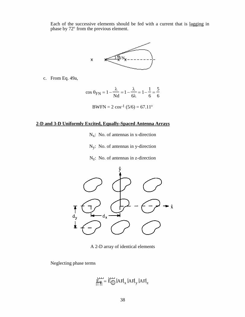
BWFN = 2 cos-1 (5/6) = 67.11° 2-D and 3-D Uniformly Excited, Equally-Spaced Antenna Arrays Nx: No. of antennas in x-direction Ny: No. of antennas in y-direction Nz: No. of antennas in z-direction

A 2-D array of identical elements Neglecting phase terms

E T =

E 1 AF x AF y AF z

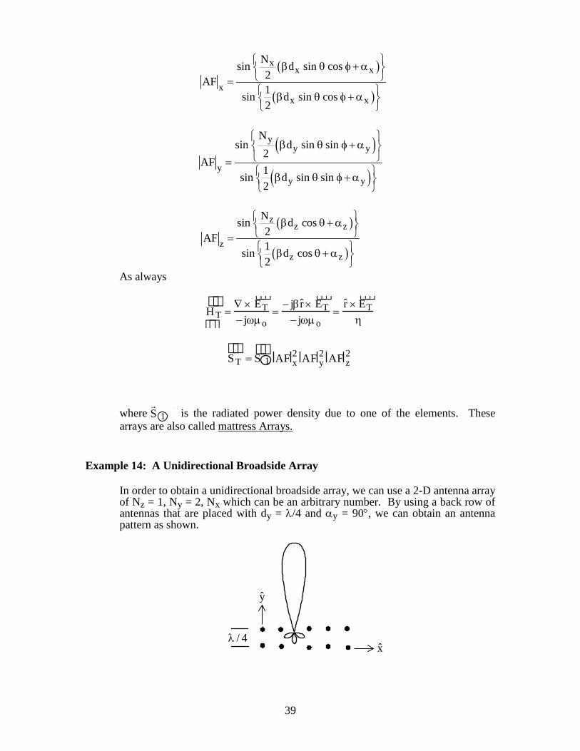
39

( )

( )

xx x

xx x

Nsin d sin cos2AF1sin d sin cos2

β θ φ + α = β θ φ + α

( )

( )

yy y

yy y

Nsin d sin sin

2AF

1sin d sin sin2

β θ φ + α

= β θ φ + α

( )

( )

zz z

zz z

Nsin d cos2AF1sin d cos2

β θ + α = β θ + α

As always

H T =

∇ ×E T

− jωµo=

− jβˆ r ×E T

− jωµo=

ˆ r ×E T

η

T =

1 AF x

2 AF y2 AF z

2S S

where S 1 is the radiated power density due to one of the elements. These

arrays are also called mattress Arrays. Example 14: A Unidirectional Broadside Array In order to obtain a unidirectional broadside array, we can use a 2-D antenna array

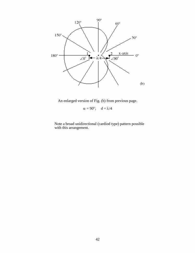
of Nz = 1, Ny = 2, Nx which can be an arbitrary number. By using a back row of antennas that are placed with dy = λ/4 and αy = 90°, we can obtain an antenna pattern as shown.

S

1

/ 4λ x

y

40

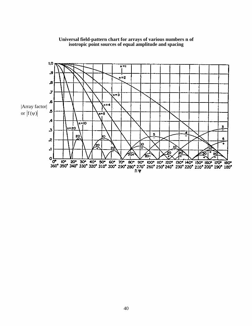
Universal field-pattern chart for arrays of various numbers n of isotropic point sources of equal amplitude and spacing

|Array factor| or f ( )ψ

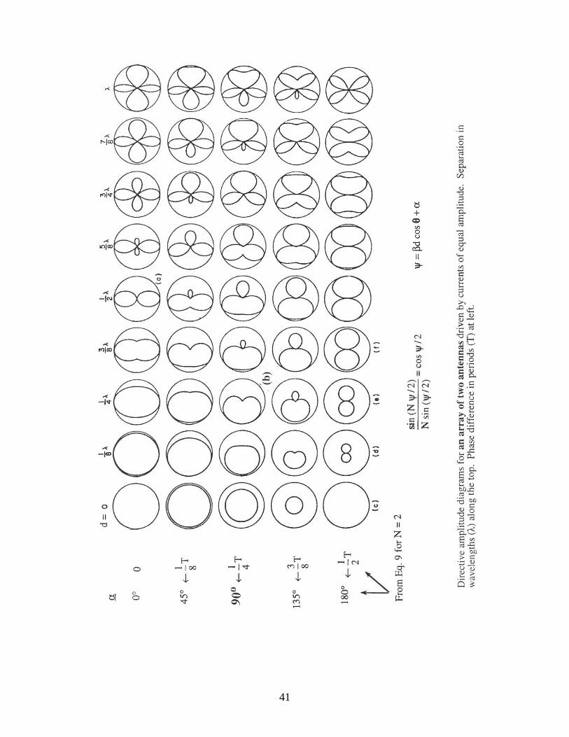
41

42

An enlarged version of Fig. (b) from previous page. α = 90°; d = λ/4 Note a broad unidirectional (cardiod type) pattern possible with this arrangement.

0∠ 90∠

43

Reactance of Linear Dipoles We have previously calculated Rin = Ra + Rohmic for linear dipole or monopole

antennas. We need to know the input reactance Xin or Xa in order to design matching networks to match power in or out of the antenna.

Like the current distribution on a linear dipole, the input reactance can be written

as though a two-wire line of length L/2 had been opened up as shown in the following:

dD

S

E

L/2

′ D ′ E E

D

′ D

′ E

S(z)

L/2

E

L/2

D

′ D

′ E

z = 0g/2

-g/22 ′ z

′ z

− ′ z

a.

b. c.

For a two-wire line of Fig. a, each of diameter d,

• or

120 2SZ nd

= ε (1)

For the opened-up line of Fig. b, we can define an average characteristic

impedance Z o

• L / 2

o o0

1Z Z (z) dzL / 2

= ∫ (2)

44

For the completely opened-up transmission line of Fig. c, we can define

g / 2 L / 2

oarg / 2

r

2 120 4zZ n dzL d

120 2Ln 1d

+ ′ ′= ε

= − ε

∫

(3)

The reactance ZD ′ D of an open-circuited transmission line of length L/2 can be

written from Transmission Line Theory

DD in oaLZ Z jZ cot2′

= = − β

(4)

Combining Eq. 3 and 4, we can write

DD in oaLZ jX j Z cot2′

′β = = −

(5)

where L (1.02 1.10)L′ ≅ − is the effective "electrical" length of the antenna. Reactance of Linear Monopoles Above Ground We have previously shown that Rin monopole

=12

Rin dipole (6)

Similarly,

dipolemonopole

oa oa1 2LZ Z 60 n 12 d

= = −

(7)

From Eq. 5

monopole dipolein in

1X X2

= (8)

Example 15: Calculate the feed point impedances Rin + jXin for linear dipoles of length (a) L =

0.5λ (half wave dipole) and (b) L = 0.3λ. Assume that the antenna wire is No. 19 AWG (d = 9.12 × 10-4 m from Table B.2, p. 623) and frequency f = 30 MHz. Take copper as the material for the antenna.

45

a. From the table on driving point resistance, p. 7 of Class Notes

L / 2 0.25riR 2 36.56 73.12λ=

= × = Ω (9)

From p.13 of Class Notes, Eq. 9

sohmic

2

R 1 L sin ( L)Ra 4 4sin

2

β= − ππ β

(10)

σcopper = 5.8 × 107 S/m

4s MHz

1R 2.61 10 f−= = ×σδ

for copper

4 4sR 2.6 10 30 14.4 10 @ f 30 MHz− −= × = × Ω = (11)

L =λ2

= 5 m

Rohmic =14.4 ×10−4

π × 4.06 ×10−454

=1.411Ω (12)

Rin = Rri + Rohmic = 74.53Ω (13) From Eq. 3 on p. 44 of Class Notes

oa 410Z 120 n 1 996.3

9.25 10−

= − = Ω ×

(14)

Taking ′ L ≅ 1.02 L = 0.51λ

2 0.510cot 0.0314

2π λ × = − λ

From Eq. 5 on p. 44 of Class Notes

inLjX j 996.3 cot j 31.32

′β = − = + Ω

(15)

Zin = Rin + jX in = 74.53 + j31.3Ω (16)

46

Note that if we had constructed a slightly shorter, say L = 0.49λ dipole ′ L = 0.49 ×1.02λ = 0.5λ jX in = −j 996.3 cot β ′ L ⇒ 0 Zin = Rri + Rohmic + j0 = 69.46 +1.41+ j0 ≅ 71 + j0Ω (17) b. You can solve for the numbers for part b of the problem following the procedure

indicated above. Example 16: Feedpoint impedance for a linear monopole of length L/2 = 0.25λ. Solution: From Eq. 16 Zin monopole

=12

Zin dipole= 37.27 + j15.65Ω

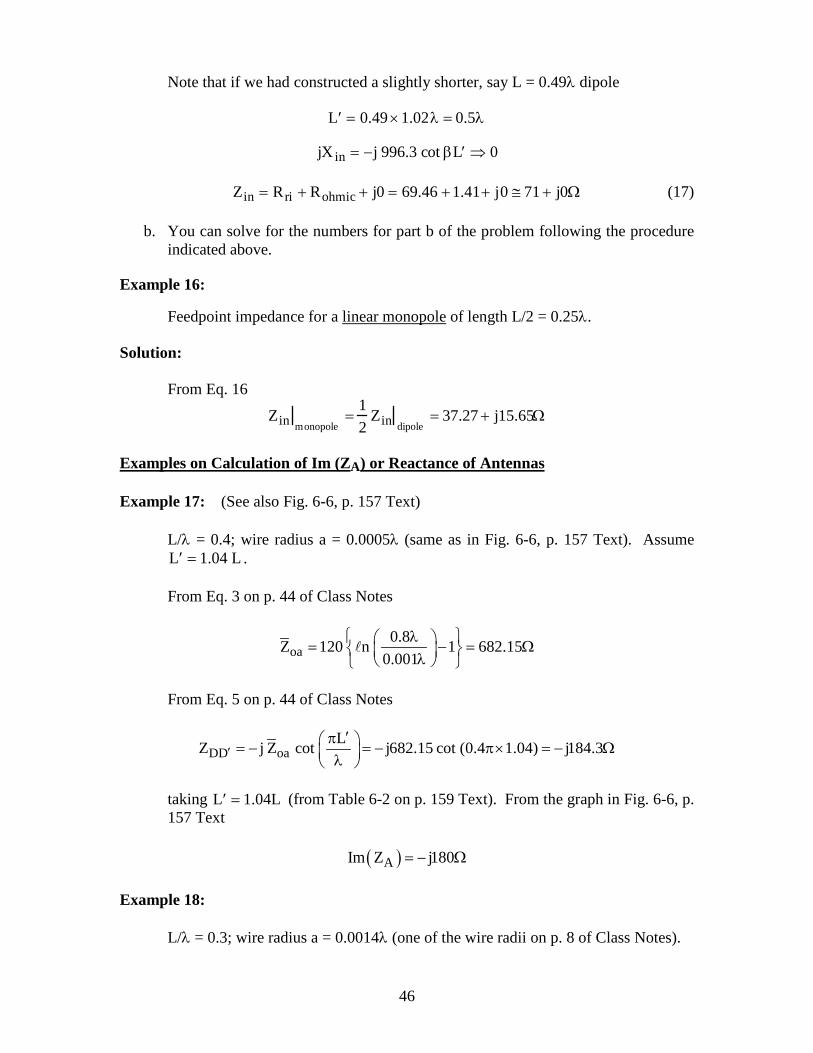
Examples on Calculation of Im (ZA) or Reactance of Antennas Example 17: (See also Fig. 6-6, p. 157 Text) L/λ = 0.4; wire radius a = 0.0005λ (same as in Fig. 6-6, p. 157 Text). Assume

′ L = 1.04 L . From Eq. 3 on p. 44 of Class Notes

oa0.8Z 120 n 1 682.15

0.001 λ = − = Ω λ

From Eq. 5 on p. 44 of Class Notes

DD oaLZ j Z cot j682.15 cot (0.4 1.04) j184.3′

′π = − = − π× = − Ω λ

taking ′ L = 1.04L (from Table 6-2 on p. 159 Text). From the graph in Fig. 6-6, p.

157 Text ( )AIm Z j180= − Ω Example 18: L/λ = 0.3; wire radius a = 0.0014λ (one of the wire radii on p. 8 of Class Notes).

47

From Eq. 3, p. 44 of Class Notes

oa0.6Z 120 n 1 524.08

0.0028 λ = − = Ω λ

DDLZ j524.08 cot L j524.08 cot 0.3 j351.4L′′π ′= − = − π× = − Ω λ

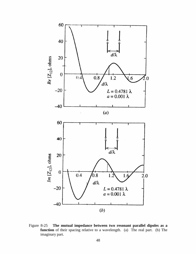
taking L / L 1.04′ = . From graph on p. 8 of Class Notes Reactance Xa = −2 ×150 = −300Ω which is close. Examples on Mutual Impedance Effects Example 19: A half-wave dipole above ground Distance to ground gd / 4= λ g2d = distance to image antenna2 = / 2λ From Fig. 8-25a, b, for d/λ = 0.5 12Z 12.5 j30;= − − 2 1 1I I 180 I= ∠ = − [ ]1 1 11 2 12 1 11 12V I Z I Z I Z Z= + = −

1

11

VZ (73 j42.5) ( 12.5 j30)I

85.5 j72.5

= = + − − −

= +

Feedpoint impedance of the half-wave dipole placed at a distance of / 4λ from

the ground = 85.5 + j72.5Ω rather than 73 + j42.5Ω . Radiation Pattern We can consider the above situation as a 2-element (N = 2) antenna array in the x

direction and write

T 1E E AF=

gd

x

z 1

1

gd 2 Image

antenna

48

Figure 8-25 The mutual impedance between two resonant parallel dipoles as a function of their spacing relative to a wavelength. (a) The real part. (b) The imaginary part.

49

Figure 8-26 The mutual impedance between two resonant collinear dipoles as a

function of spacing relative to a wavelength. (a) The real part. (b) The imaginary part.

50

( )( )

sin N / 2AF

sin / 2ψ

=ψ

where

x x gd sin cos 2 d sin cos

sin cos

ψ = β θ φ + α = β θ φ + π

= π θ φ + π

From pp. 36-37 of Class Notes, Eqs. (54)-(57)

2 A,isolated 2o max

A,with ground effect

R 73D G D AF 1.64 N 4 5.60R 85.5

= = = × × =

Without ground effect

D = G = 1.64

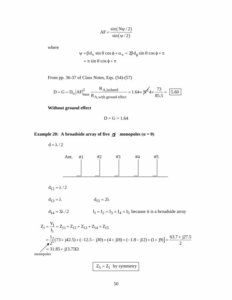
Example 20: A broadside array of five λ/4 monopoles (α = 0) d / 2= λ

12d / 2= λ 13d = λ 15d 2= λ 14d 3 / 2= λ 1 2 3 4 5I I I I I= = = = because it is a broadside array

[ ]

11 11 12 13 14 15

1

VZ Z Z Z Z ZI1 63.7 j27.5(73 j42.5) ( 12.5 j30) (4 j18) ( 1.8 j12) (1 j9)2 231.85 j13.75

= = + + + +

+= + + − − + + + − − + + =

= + Ω

5 1Z Z= by symmetry

Ant. #1 #2 #3 #4 #5

monopoles

51

[ ]

[ ]

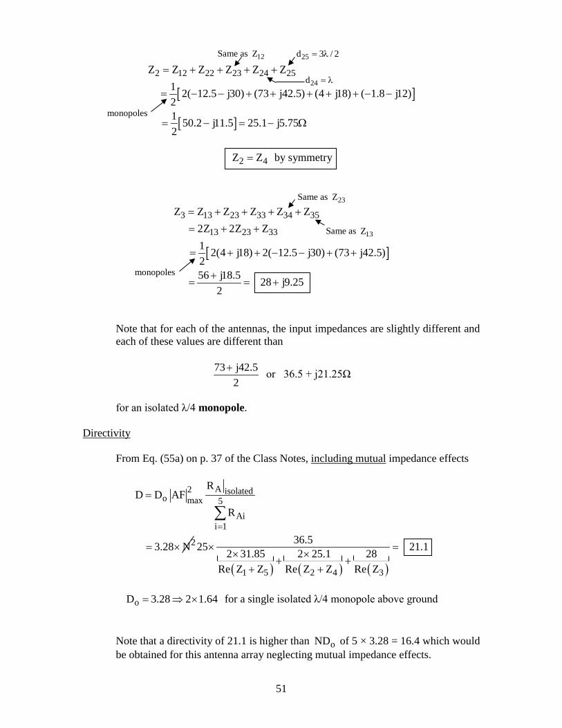
2 12 22 23 24 25Z Z Z Z Z Z1 2( 12.5 j30) (73 j42.5) (4 j18) ( 1.8 j12)21 50.2 j11.5 25.1 j5.752

= + + + +

= − − + + + + + − −

= − = − Ω

2 4Z Z= by symmetry

[ ]

3 13 23 33 34 35

13 23 33

Z Z Z Z Z Z2Z 2Z Z1 2(4 j18) 2( 12.5 j30) (73 j42.5)256 j18.5 28 j9.25

2

= + + + +

= + +

= + + − − + +

+= = +

Note that for each of the antennas, the input impedances are slightly different and each of these values are different than

73 j42.5

2+ or 36.5 + j21.25Ω

for an isolated λ/4 monopole. Directivity From Eq. (55a) on p. 37 of the Class Notes, including mutual impedance effects

( ) ( ) ( )

A2 isolatedo max 5

Aii 1

2

1 5 2 4 3

RD D AF

R

36.53.28 N 25 21.12 31.85 2 25.1 28Re Z Z Re Z Z Re Z

=

=

= × × =× ×

+ ++ +

∑

oD 3.28 2 1.64= ⇒ × for a single isolated λ/4 monopole above ground

Note that a directivity of 21.1 is higher than oND of 5 × 3.28 = 16.4 which would be obtained for this antenna array neglecting mutual impedance effects.

monopoles

Same as 12Z

24d = λ

monopoles

Same as 23Z

Same as 13Z

25d 3 / 2= λ

52

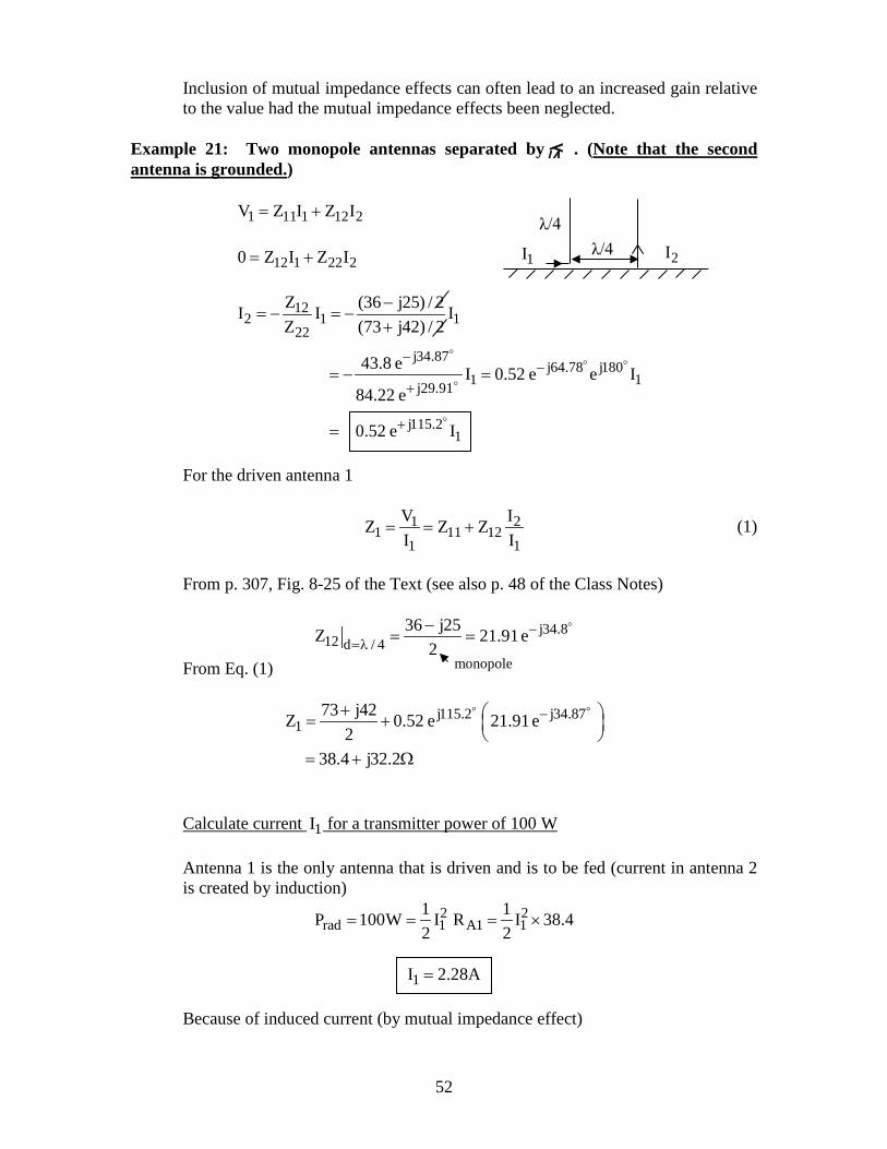
Inclusion of mutual impedance effects can often lead to an increased gain relative to the value had the mutual impedance effects been neglected.

Example 21: Two monopole antennas separated by λ/4 . (Note that the second antenna is grounded.) 1 11 1 12 2V Z I Z I= + 12 1 22 20 Z I Z I= +

122 1 1

22

j34.87j64.78 j180

1 1j29.91

j115.21

Z (36 j25) / 2I I IZ (73 j42) / 2

43.8 e I 0.52 e e I84.22 e

0.52 e I

−−

+

+

−= − = −

+

= − =

=

For the driven antenna 1

1 21 11 12

1 1

V IZ Z ZI I

= = + (1)

From p. 307, Fig. 8-25 of the Text (see also p. 48 of the Class Notes)

j34.812 d / 4

36 j25Z 21.91e2

−=λ

−= =

From Eq. (1)

j115.2 j34.871

73 j42Z 0.52 e 21.91e2

38.4 j32.2

−+ = +

= + Ω

Calculate current 1I for a transmitter power of 100 W Antenna 1 is the only antenna that is driven and is to be fed (current in antenna 2

is created by induction)

2 2rad 1 A1 1

1 1P 100W I R I 38.42 2

= = = ×

1I 2.28A= Because of induced current (by mutual impedance effect)

λ/4 λ/4

1I 2I

monopole

53

j115.2 j115.22 1I 0.52 I e 1.19 e A= × =

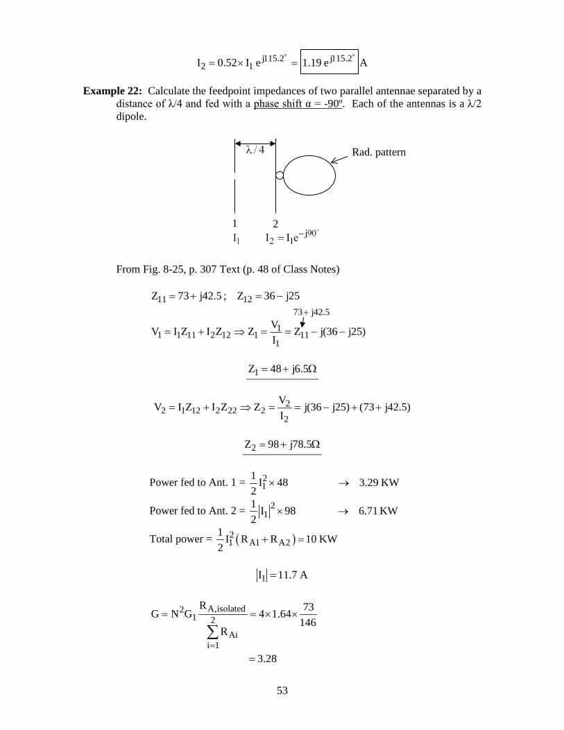
Example 22: Calculate the feedpoint impedances of two parallel antennae separated by a

distance of λ/4 and fed with a phase shift α = -90º. Each of the antennas is a λ/2 dipole.

From Fig. 8-25, p. 307 Text (p. 48 of Class Notes)

11 12Z 73 j42.5 ; Z 36 j25= + = −

11 1 11 2 12 1 11

1

VV I Z I Z Z Z j(36 j25)I

= + ⇒ = = − −

1Z 48 j6.5= + Ω

22 1 12 2 22 2

2

VV I Z I Z Z j(36 j25) (73 j42.5)I

= + ⇒ = = − + +

2Z 98 j78.5= + Ω

Power fed to Ant. 1 = 21

1 I 482

× 3.29 KW→

Power fed to Ant. 2 = 21

1 I 982

× 6.71 KW→

Total power = ( )21 A1 A2

1 I R R 10 KW2

+ =

1I 11.7 A=

A,isolated21 2

Aii 1

R 73G N G 4 1.64146

R

3.28=

= = × ×

=

∑

1 2

73 j42.5+

Rad. pattern

54

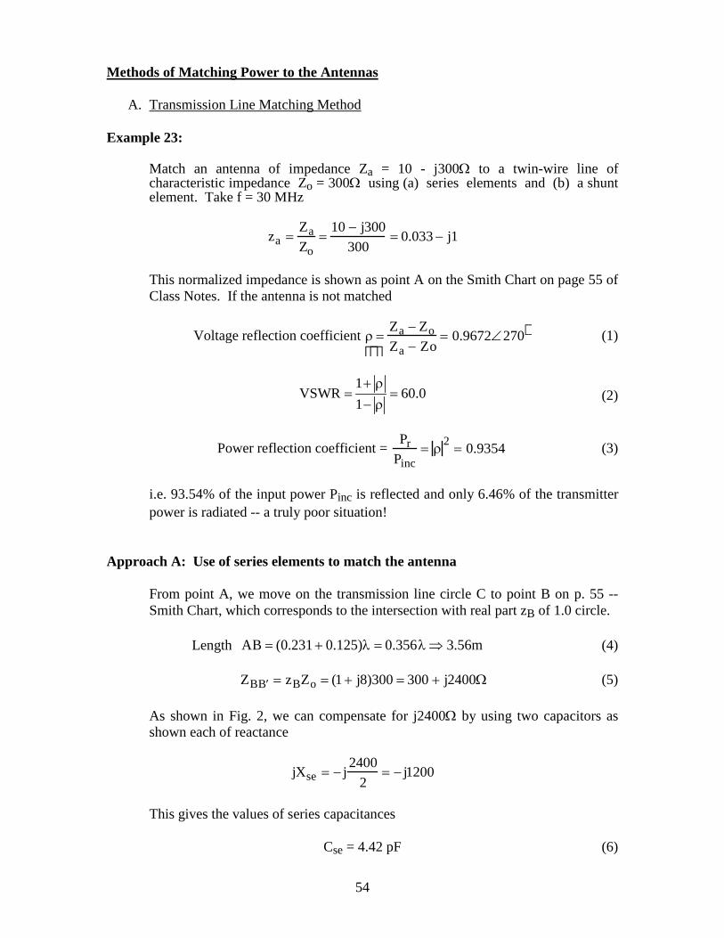
Methods of Matching Power to the Antennas A. Transmission Line Matching Method Example 23: Match an antenna of impedance Za = 10 - j300Ω to a twin-wire line of

characteristic impedance Zo = 300Ω using (a) series elements and (b) a shunt element. Take f = 30 MHz

za =

ZaZo

=10 − j300

300= 0.033 − j1

This normalized impedance is shown as point A on the Smith Chart on page 55 of

Class Notes. If the antenna is not matched Voltage reflection coefficient

ρ =

Za − ZoZa − Zo

= 0.9672∠270 (1)

1

VSWR 60.01

+ ρ= =

− ρ (2)

Power reflection coefficient = Pr

Pinc= ρ 2 = 0.9354 (3)

i.e. 93.54% of the input power Pinc is reflected and only 6.46% of the transmitter

power is radiated -- a truly poor situation! Approach A: Use of series elements to match the antenna From point A, we move on the transmission line circle C to point B on p. 55 --

Smith Chart, which corresponds to the intersection with real part zB of 1.0 circle. Length AB = (0.231 + 0.125)λ = 0.356λ ⇒ 3.56m (4) ZB ′ B = zBZo = (1 + j8)300 = 300 + j2400Ω (5) As shown in Fig. 2, we can compensate for j2400Ω by using two capacitors as

shown each of reactance jXse = − j

24002

= − j1200

This gives the values of series capacitances Cse = 4.42 pF (6)

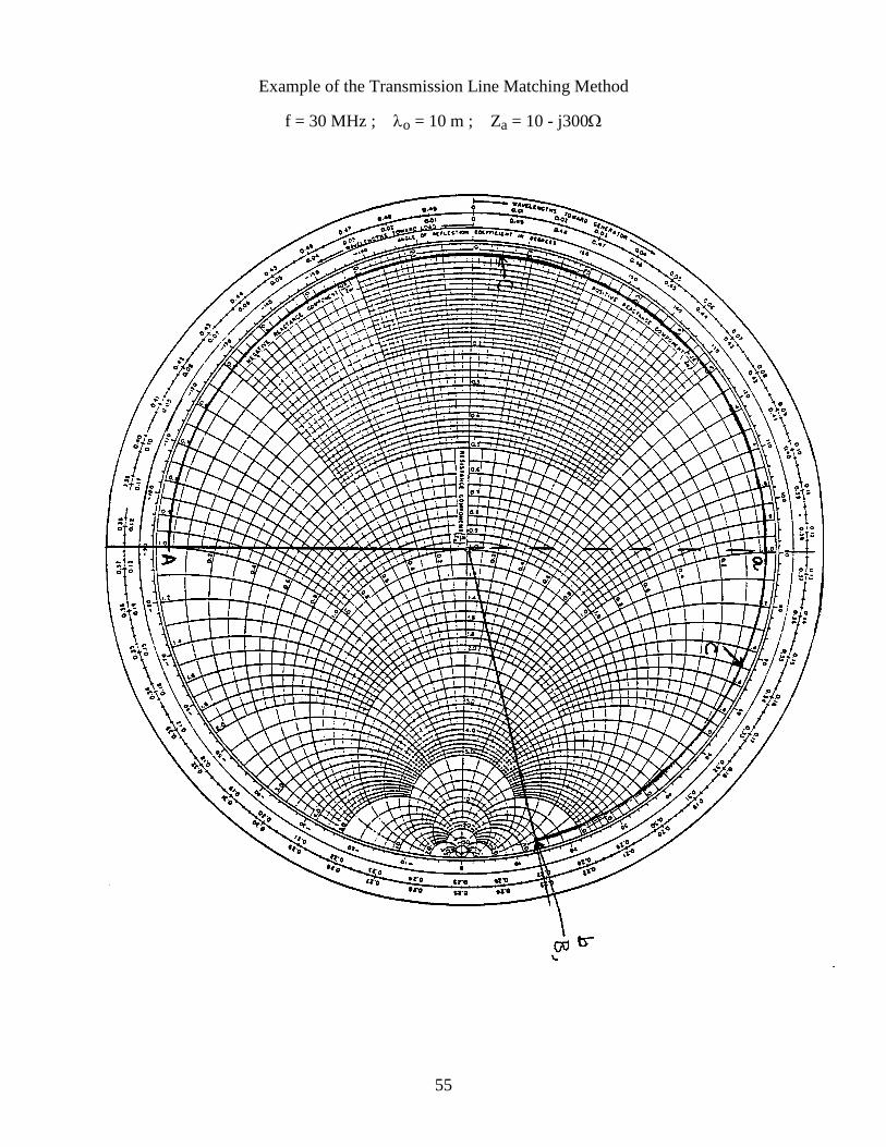
55

Example of the Transmission Line Matching Method f = 30 MHz ; λo = 10 m ; Za = 10 - j300Ω

56

Fig. 2. Approach B: An alternative design using a shunt element to match the antenna An undesirable feature of the above design Approach A is that it takes a fairly

long length AB = 0.356λ over which the transmission line is not matched. For the alternative Approach B, we work in terms of admittances.

YA =

110 − j300

; yA =1

0.033 − j1≅ 0.033 + j1 (7)

This is shown by point a on the Smith Chart on page 55. Now, we need to move only a distance ab = (0.231− 0.125)λ = 0.106λ = 1.06 m (8) and use (as sketched in Fig. 3) a shunt element to match the line.

Fig. 3.

− j Ysh = − j8

300mho ⇒ −

jω Lsh

(9)

Lsh =300

8 × 2π × 30 ×106 = 0.2 µH (10)

57

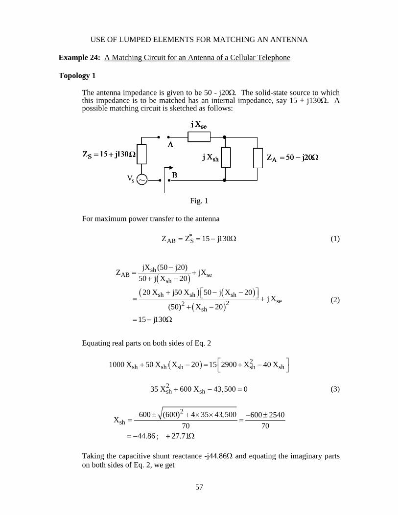
USE OF LUMPED ELEMENTS FOR MATCHING AN ANTENNA Example 24: A Matching Circuit for an Antenna of a Cellular Telephone Topology 1 The antenna impedance is given to be 50 - j20Ω. The solid-state source to which

this impedance is to be matched has an internal impedance, say 15 + j130Ω. A possible matching circuit is sketched as follows:

Fig. 1 For maximum power transfer to the antenna ZAB = ZS

∗ = 15 − j130Ω (1)

( )( ) ( )

( )

shAB se

sh

sh sh shse22

sh

jX (50 j20)Z jX50 j X 20

20 X j50 X 50 j X 20j X

(50) X 2015 j130

−= +

+ −

+ − − = ++ −

= − Ω

(2)

Equating real parts on both sides of Eq. 2

( ) 2sh sh sh sh sh1000 X 50 X X 20 15 2900 X 40 X + − = + −

35 Xsh

2 + 600 Xsh − 43,500 = 0 (3)

2

sh600 (600) 4 35 43,500 600 2540X

70 7044.86 ; 27.71

− ± + × × − ±= =

= − + Ω

Taking the capacitive shunt reactance -j44.86Ω and equating the imaginary parts

on both sides of Eq. 2, we get

sV

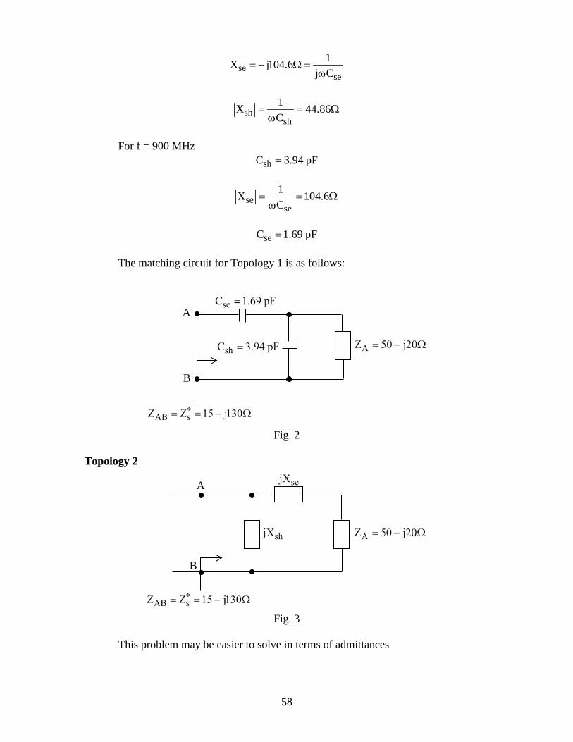
58

sese

1X j104.6j C

= − Ω =ω

shsh

1X 44.86C

= = Ωω

For f = 900 MHz

shC 3.94 pF=

sese

1X 104.6C

= = Ωω

seC 1.69 pF=

The matching circuit for Topology 1 is as follows:

Fig. 2

Topology 2

Fig. 3

This problem may be easier to solve in terms of admittances

A

B

A

B

59

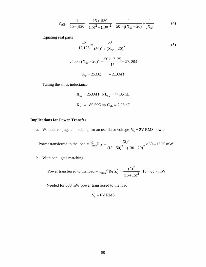
AB 2 2 se sh

1 15 j130 1 1Y15 j130 50 j(X 20) jX(15) (130)

+= = = +

− + −+ (4)

Equating real parts

2 2se

15 5017,125 (50) (X 20)

=+ −

(5)

2

se50 171252500 (X 20) 57,083

15×

+ − = =

eX 253.6; 213.6= − Ω

Taking the sines inductance

se seX 253.6 L 44.85 nH= Ω ⇒ =

sh shX 85.59 C 2.06 pF= − Ω ⇒ =

Implications for Power Transfer a. Without conjugate matching, for an oscillator voltage sV 2V= RMS power

Power transferred to the load = 2

2rms A 2 2

(2)I R 50 12.25 mW(15 50) (130 20)

= × =+ + −

b. With conjugate matching

Power transferred to the load = 2

2rms s 2

(2)I Re Z 15 66.7 mW(15 15)

∗′ = × =+

Needed for 600 mW power transferred to the load

sV 6V RMS=

60

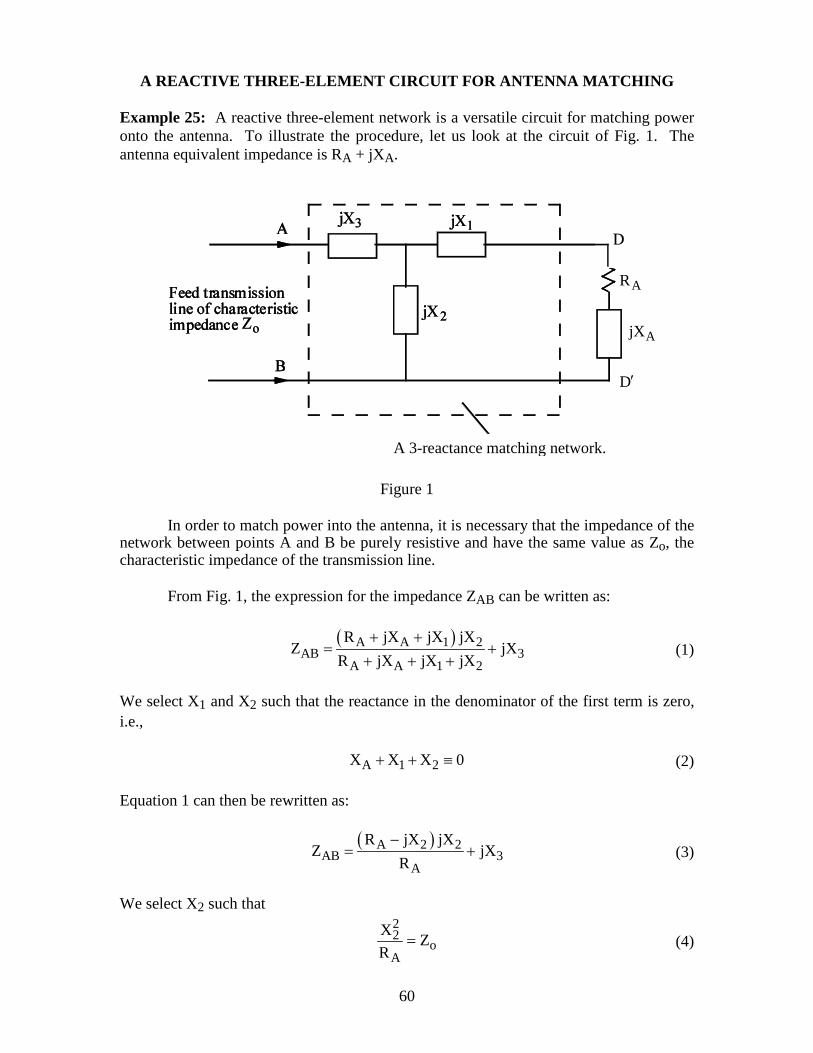
A REACTIVE THREE-ELEMENT CIRCUIT FOR ANTENNA MATCHING Example 25: A reactive three-element network is a versatile circuit for matching power onto the antenna. To illustrate the procedure, let us look at the circuit of Fig. 1. The antenna equivalent impedance is RA + jXA.

Figure 1 In order to match power into the antenna, it is necessary that the impedance of the network between points A and B be purely resistive and have the same value as Zo, the characteristic impedance of the transmission line. From Fig. 1, the expression for the impedance ZAB can be written as:

( )A A 1 2

AB 3A A 1 2

R jX jX jXZ jX

R jX jX jX+ +

= ++ + +

(1)

We select X1 and X2 such that the reactance in the denominator of the first term is zero, i.e., A 1 2X X X 0+ + ≡ (2) Equation 1 can then be rewritten as:

( )A 2 2

AB 3A

R jX jXZ jX

R−

= + (3)

We select X2 such that

22

oA

X ZR

= (4)

A 3-reactance matching network.

AjX

AR

D′

61

and X3 such that X3 = -X2 (5) This would then give ZAB = Zo + j0 and the antenna would then be matched onto the transmission line. To illustrate the procedure by a numerical example, let us say that the antenna is a monopole and its impedance AZ has been calculated and found to be 1.5 - j460Ω. Let us take Zo = 300 ohms (we must, of course, make sure that the diameter of the feeder line is not overly thin for the current-carrying requirement). From Eq. 4, 2X 1.5 300 21.2= ± × = ± Ω (6) The upper sign corresponds to an inductance L = 21.1/ω and the lower sign corresponds to a capacitance

C =1

ω × 21.2 .

We can use either type. Case 1: For inductive element X2 2 2jX j L j21.2= ω = Ω If ω is prescribed, 2L can be calculated. From Eq. 2, X1 = - X2 - XA = -21.2 + 460 = 438.8Ω This implies an inductor for 1jX . From Eq. 5, X3 = - 21.2Ω One possible 3-reactance matching network is, therefore, shown in Fig. 2.

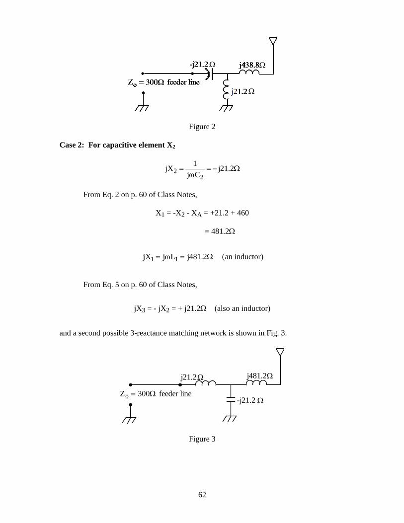
62

Figure 2 Case 2: For capacitive element X2

22

1jX j21.2j C

= = − Ωω

From Eq. 2 on p. 60 of Class Notes, X1 = -X2 - XA = +21.2 + 460 = 481.2Ω

1 1jX j L j481.2= ω = Ω (an inductor)

From Eq. 5 on p. 60 of Class Notes, jX3 = - jX2 = + j21.2Ω (also an inductor) and a second possible 3-reactance matching network is shown in Fig. 3.

Zo = 300Ω feeder line

j481.2

-j21.2

j21.2

Figure 3

Ω

Ω

Ω

Ω

Ω Ω

63

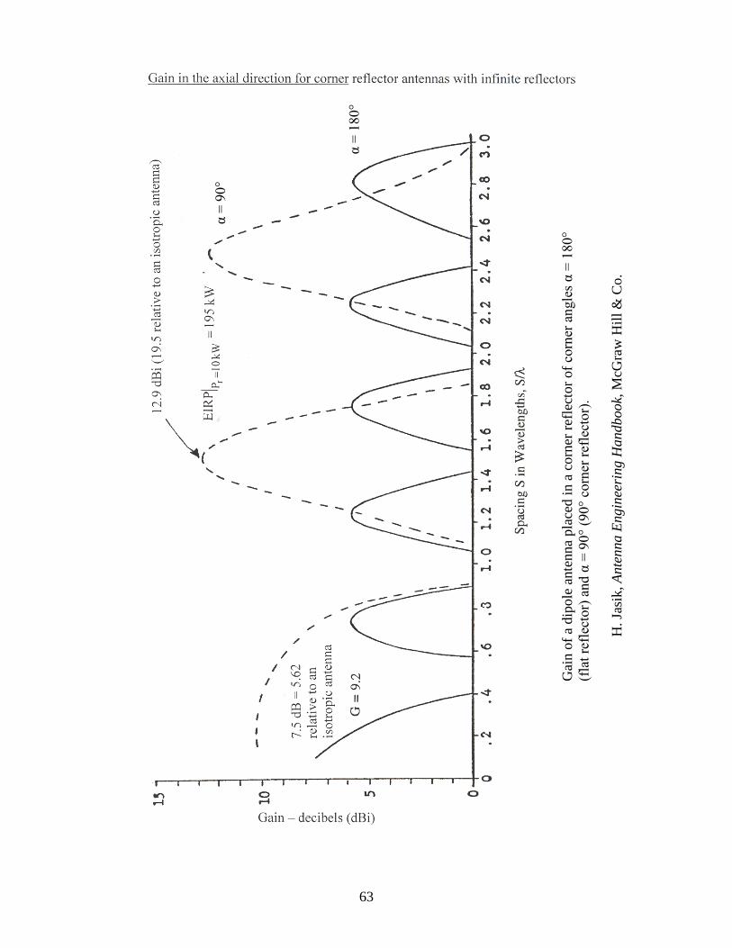
Gai

n of

a d

ipol

e an

tenn

a pl

aced

in a

cor

ner r

efle

ctor

of c

orne

r ang

les α

= 1

80°

(fla

t ref

lect

or) a

nd α

= 9

0° (9

0° c

orne

r ref

lect

or).

H

. Jas

ik, A

nten

na E

ngin

eeri

ng H

andb

ook,

McG

raw

Hill

& C

o.

α =

90°

α =

180°

64

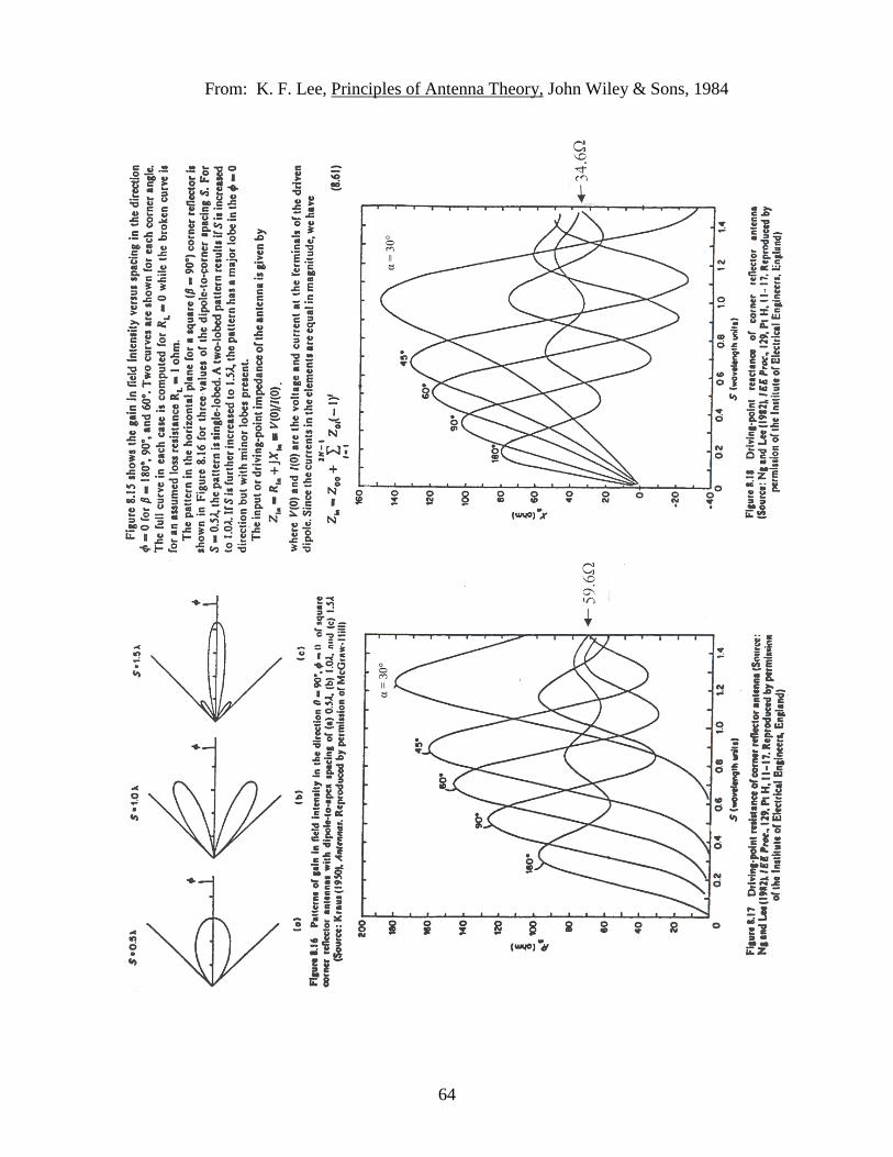
From: K. F. Lee, Principles of Antenna Theory, John Wiley & Sons, 1984

α =

30°

α =

30°

65

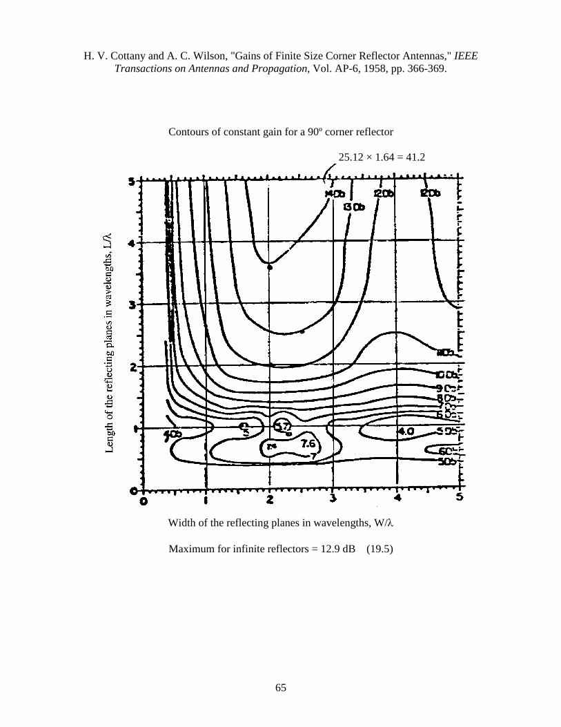
H. V. Cottany and A. C. Wilson, "Gains of Finite Size Corner Reflector Antennas," IEEE Transactions on Antennas and Propagation, Vol. AP-6, 1958, pp. 366-369.

Contours of constant gain for a 90º corner reflector 25.12 × 1.64 = 41.2

Width of the reflecting planes in wavelengths, W/λ Maximum for infinite reflectors = 12.9 dB (19.5)

66

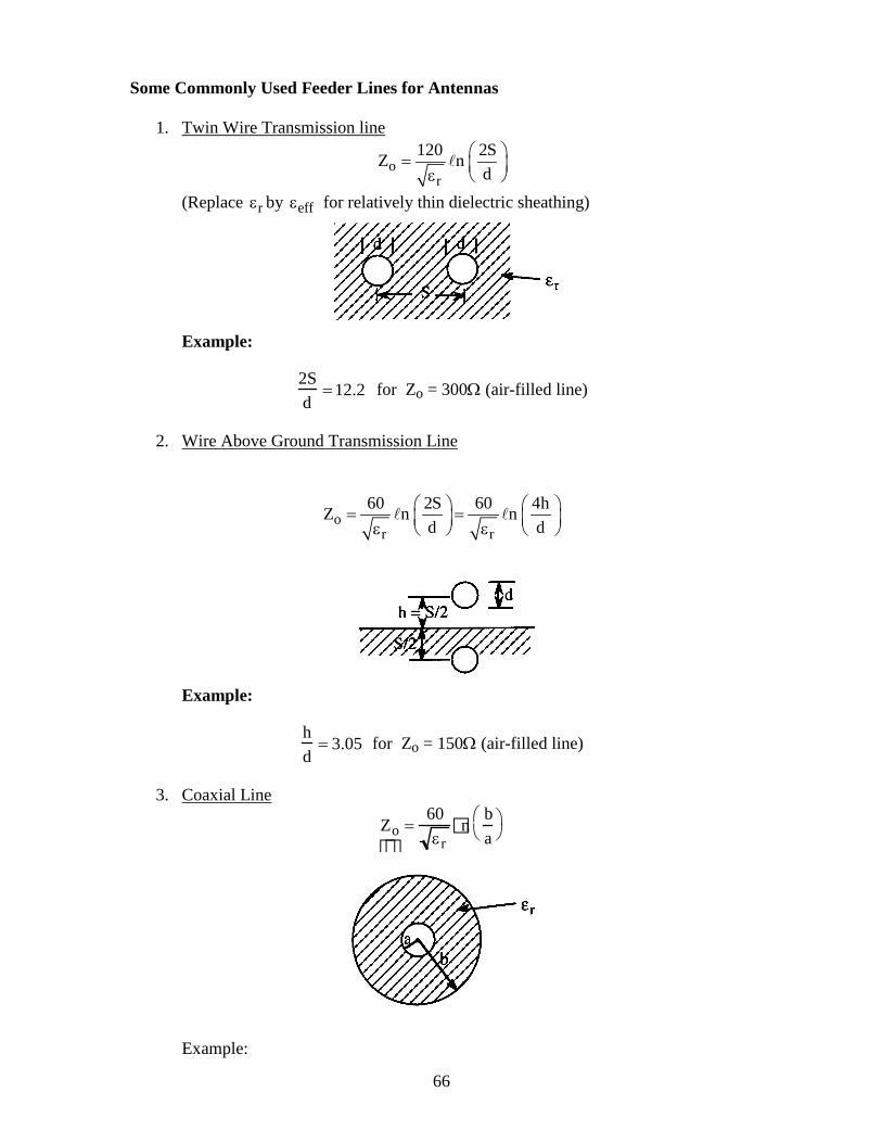
Some Commonly Used Feeder Lines for Antennas 1. Twin Wire Transmission line

or

120 2SZ nd

= ε

(Replace rε by effε for relatively thin dielectric sheathing)

Example: 2S

d=12.2 for Zo = 300Ω (air-filled line)

2. Wire Above Ground Transmission Line

or r

60 2S 60 4hZ n nd d

= = ε ε

Example: h

d= 3.05 for Zo = 150Ω (air-filled line)

3. Coaxial Line

Zo =60εr

nba

Example:

67

b

a= 3.345 for εr = 2.1 (Teflon) coaxial line of Zo = 50Ω

Some of the other transmission lines useful for printed antennas are: a. Miscrostripline b. Slot line etc. Ground Effect on Radiation Pattern of an Antenna We have previously considered the effect of ground for the radiation from a

vertical monopole antenna. The net effect was that the monopole antenna of length L/2 radiates electromagnetic fields much like a dipole of length L albeit for the upper half plane i.e. for field points above ground.

For a horizontal dipole antenna placed at a distance h from the ground as sketched

in Fig. 1, an image antenna ′ 1 is created, which has a current excitation that is equal in magnitude (for high conductivity ground) but 180º out of phase with that in the installed antenna #1.

Fig. 1. A horizontal dipole antenna above ground. From Eq. 10 on p. 24 of the Class Notes, this can be considered as a two-element

array (Ny = 2) with a phase difference αy = π or 180º.

90 − φ

68

( )

( )

T 1 1 1y

1

sin 212E E AF E E 2 cos 2 h sin sin2sin

2E 2 sin h sin sin

ψ = = = β θ φ + π ψ

= β θ φ

neglecting the phase factors both in writing |AF|y and

E 1. Note that Eq. 1 could

also have been written by following a procedure similar to that for Eq. 4 on page 24 of the Class Notes.

( ) ( )

( )

1 1j r r j 2h sin sinT 1 i 1 1

j h sin sin j h sin sin1 1

E E E E 1 e E 1 e

E e e 2 E sin h sin sin

′− β − − β θ φ

− β θ φ − β θ φ

= + = − = − = − = β θ φ

ignoring the phase factors, as also done in writing Eq. 1. From Eqs. 1 and 2 ( ) ( )AF 2 sin h sin sin 2 sin h sin= β θ φ ⇒ β φ (3) for θ = π/2 i.e. xy plane. For maxima of radiation

βh sin φo = ±

π2

, ± 3π2

, (4)

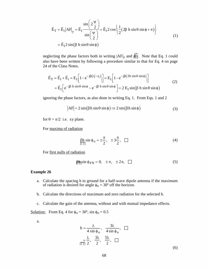
For first nulls of radiation βh sin φFN = 0, ± π, ± 2π, (5) Example 26 a. Calculate the spacing h to ground for a half-wave dipole antenna if the maximum

of radiation is desired for angle φo = 30º off the horizon. b. Calculate the directions of maximum and zero radiation for the selected h. c. Calculate the gain of the antenna, without and with mutual impedance effects. Solution: From Eq. 4 for φo = 30º, sin φo = 0.5 a.

h = λ4 sin φo

, 3λ4 sin φo

,

=λ2

,3λ2

,5λ2

,

(6)

(1)

(2)

69

In order to keep the number of principal maxima to a minimum number, we select

the smallest spacing to the ground plane i.e. h = λ/2 (7) b. For this spacing itself, we note from Eq. 4 that the directions of maximum

radiation are: βh sin φo = π sin φo = +

π2

(8)

φo = 30(wanted), φo = 150(unwanted) Negative sign is ignored in Eq. 8 since that gives angles φo = -30º, -150º (both

into the ground). We will see later how to eliminate the unwanted radiation for φo = 150º. If we

had taken a larger h of say 3 λ/2 from Eq. 6, we would have had many more directions of maximum radiation.

For directions of first null, from Eq. 5, φFN = 0 and sin-1(1) or 0 and 90º for the

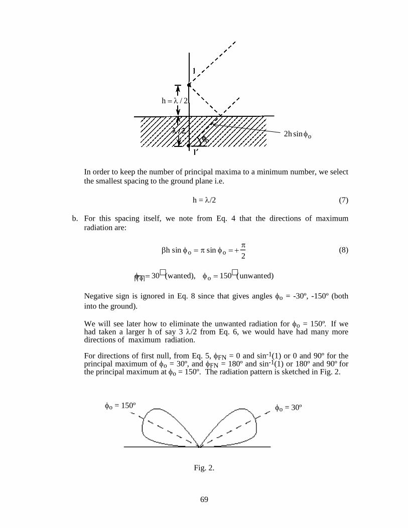
principal maximum of φo = 30º, and φFN = 180º and sin-1(1) or 180º and 90º for the principal maximum at φo = 150º. The radiation pattern is sketched in Fig. 2.

Fig. 2.

o2h sin φ οφ

h / 2= λ

φo = 150º φo = 30º

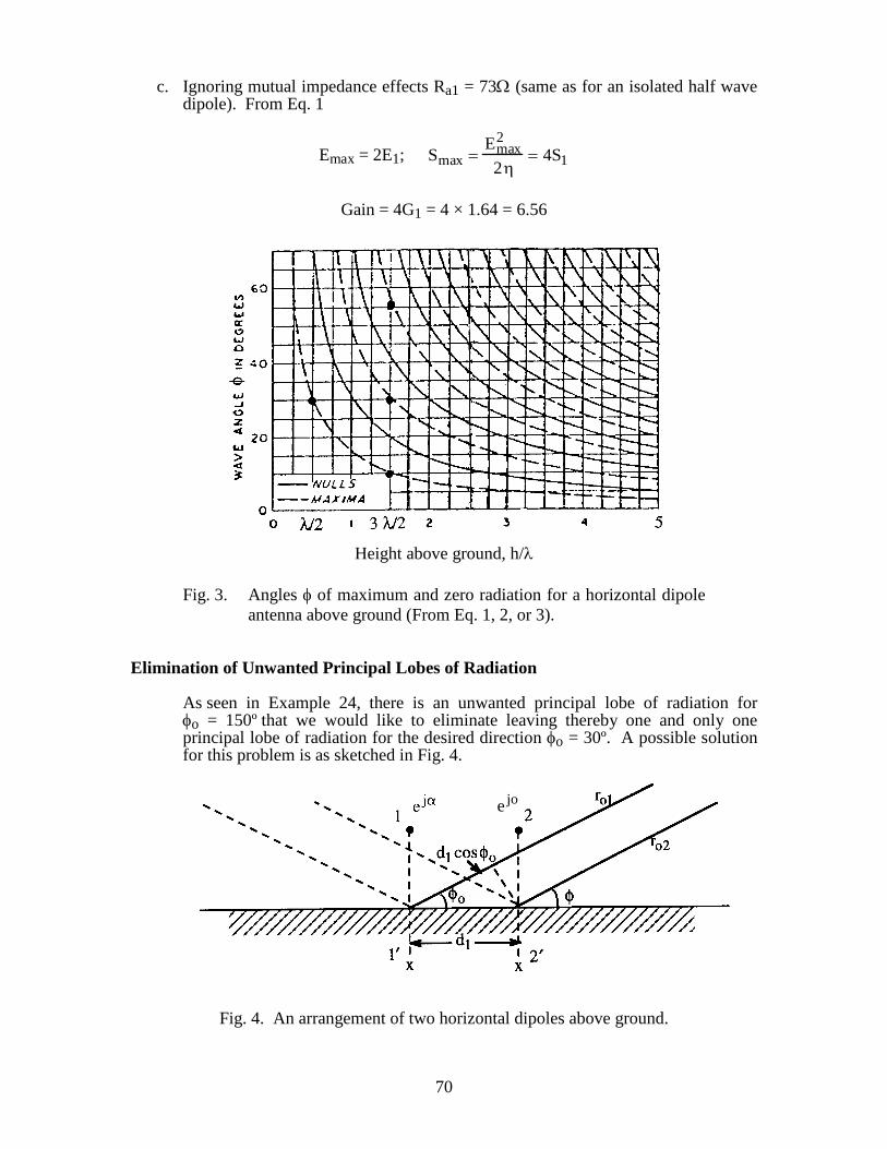
70

c. Ignoring mutual impedance effects Ra1 = 73Ω (same as for an isolated half wave dipole). From Eq. 1

Emax = 2E1; Smax =Emax

2

2η= 4S1

Gain = 4G1 = 4 × 1.64 = 6.56

Height above ground, h/λ

Fig. 3. Angles φ of maximum and zero radiation for a horizontal dipole antenna above ground (From Eq. 1, 2, or 3).

Elimination of Unwanted Principal Lobes of Radiation As seen in Example 24, there is an unwanted principal lobe of radiation for

φo = 150º that we would like to eliminate leaving thereby one and only one principal lobe of radiation for the desired direction φo = 30º. A possible solution for this problem is as sketched in Fig. 4.

Fig. 4. An arrangement of two horizontal dipoles above ground.

joe

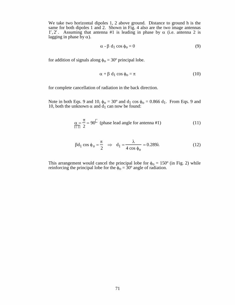
71

We take two horizontal dipoles 1, 2 above ground. Distance to ground h is the same for both dipoles 1 and 2. Shown in Fig. 4 also are the two image antennas

′ 1 , ′ 2 . Assuming that antenna #1 is leading in phase by α (i.e. antenna 2 is lagging in phase by α).

α - β d1 cos φo = 0 (9) for addition of signals along φo = 30º principal lobe. α + β d1 cos φo = π (10) for complete cancellation of radiation in the back direction. Note in both Eqs. 9 and 10, φo = 30º and d1 cos φo = 0.866 d1. From Eqs. 9 and

10, both the unknown α and d1 can now be found:

α =

π2

= 90 (phase lead angle for antenna #1) (11)

βd1 cos φo =π2

⇒ d1 =λ

4 cos φo= 0.289λ (12)

This arrangement would cancel the principal lobe for φo = 150º (in Fig. 2) while

reinforcing the principal lobe for the φo = 30º angle of radiation.

72

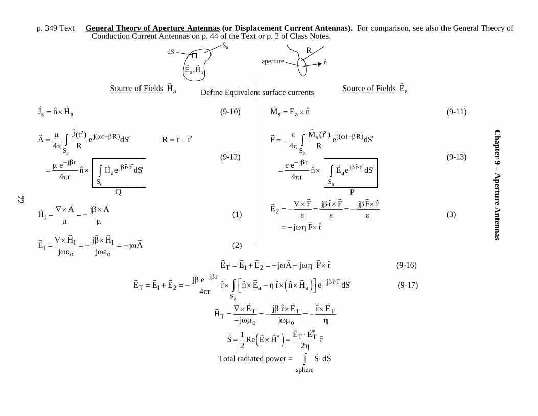
p. 349 Text General Theory of Aperture Antennas (or Displacement Current Antennas). For comparison, see also the General Theory of Conduction Current Antennas on p. 44 of the Text or p. 2 of Class Notes.

Source of Fields aH

Source of Fields aE

s aˆJ n H= ×

(9-10) s a ˆM E n= ×

(9-11)

a

a

j( t R)

Sj r

ˆj r ra

S

J(r )A e dS R r r4 R

e n H e dS4 r

ω −β

− β′β ⋅

′µ ′ ′= = −π

µ ′= ×π

∫

∫

(9-12) a

a

j( t R)s

Sj r

ˆj r ra

S

M (r )F e dS4 R

e n E e dS4 r

ω −β

− β′β ⋅

′ε ′= −π

ε ′= ×π

∫

∫

(9-13)

1A j AH ∇× β×

= = −µ µ

(1) 2ˆ ˆF j r F j F rE

ˆj F r

∇× β × β ×= − = = −

ε ε ε= − ωη ×

(3)

1 11

o o

H j HE j Aj j

∇× β×= = − = − ω

ωε ωε

(2)

T 1 2 ˆE E E j A j F r= + = − ω − ωη ×

(9-16)

( )a

j rˆj r r

T 1 2 a aS

j e ˆ ˆ ˆ ˆE E E r n E r n H e dS4 r

− β′− β ⋅β ′= + = − × × − η × × π ∫

(9-17)

T T TT

o o

ˆ ˆE j r E r EHj j

∇× β × ×= = − = −

− ωµ ωµ η

( ) T TE E1 ˆS Re E H r2 2

∗∗ ⋅

= × =η

Total radiated power = sphere

S dS⋅∫

Q P

R

aperture

Chapter 9 – A

perture Antennas

72

Define Equivalent surface currents

73

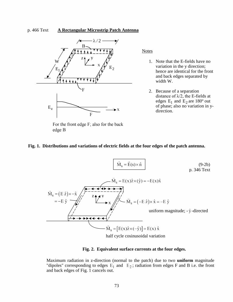
p. 466 Text A Rectangular Microstrip Patch Antenna

Fig. 1. Distributions and variations of electric fields at the four edges of the patch antenna.

z y x

uniform magnitude; - -directed

half cycle cosinusoidal variation

Fig. 2. Equivalent surface currents at the four edges.

Maximum radiation in z-direction (normal to the patch) due to two uniform magnitude "dipoles" corresponding to edges and ; radiation from edges F and B i.e. the front and back edges of Fig. 1 cancels out.

Notes

1. Note that the E-fields have no variation in the y direction; hence are identical for the front and back edges separated by width W.

2. Because of a separation

distance of λ/2, the E-fields at edges 1E and 2E are 180º out of phase; also no variation in y-direction.

W y

/ 2λ

1E 2E

zE

(9-2b) p. 346 Text

74

The array factor for the equivalent current dipoles at edges 1 2E , E can be written from Eqs. 8 and 9 on page 25 of the Class Notes. For an x-directed array of two elements N = 2; x 0α = ;

xL sin cosψ = β θ φ + α

Normalized AF =

Nsin2

2 sin2

ψ

ψ

2 sin cosL2 2 cos sin cos22 sin

2

ψ ψ β = = θ φ ψ

(1)

For a two-element (two-edge "currents") antenna array

T oE E AF=

For a uniformly-excited rectangular aperture of length W (e.g. edges 1 2E , E ), from Eqs. 9-36a, b (note that equivalent current s ˆM || y−

here rather than parallel to x on page 354 of the text)

oE E cos f ( , )θ = φ θ φ (11-5a)

oE E cos sin f ( , )φ = − θ φ θ φ (11-5b) where

Wsin sin sin2f ( , ) AFW sin sin

2Wsin sin sin

L2 cos sin cos )W 2sin sin2

β θ φ θ φ =β

θ φ

β θ φ β = θ φ β θ φ

In Eqs. 9-36a, b

z

z

Lsin u2 1L u

2

β →β

since t << λ

0

yL

thickness t

(11-5c)

75

p. 470 Text Microstrip Patch Antenna

For x-z plane ( 0φ = ) or E-plane

E

field is θ -directed with components in x- and z-directions

oE E f ( , )θ = θ φ ; Eφ = 0

For direction of maximum radiation, ˆE || x

ELF ( ) cos sin2

β θ = θ

(11-6a)

Maximum for θ = 0 i.e. along z-direction.

BWFN:

1FN

L sin sin2 2 2L

−β π λ θ = → θ =

For L2λ

, for xz or E-plane

BWFN = 12 sin2L

− λ

= 180º HPBW:

1HP

L sin sin2 4 4L

−β π λ θ = → θ =

HPBW = 1 1 12 sin 2 sin 604L 2

− −λ → →

W x . Max. rad.

L

y

76

For y-z plane ( 90φ = )

H

Wsin sin2F ( ) cos W sin

2

β θ θ = θβ

θ (11-6b)

Maximum for θ = 0

oE E cos F( , )= − θ θ φ

For yz or H-plane

1FN FN

W sin ; sin2 W

−β λ θ = π θ =

1BWFN 2sin

W− λ =

22

rA

r

LZ 901 W

ε = ε − (11-7)

for a half-wave rectangular patch antenna.

For Duroid ( rW2.2) and 2.7L

ε = =

AZ 50= Ω

1FN yz plane

1sin 47.81.35

− θ = =

BWFN = 2 1sinW

− λ

= 95.6º

HF ( )θ

77

Table 7.1. Radiation characteristics of commonly-used horn antennas.

Type of Horn

Property that is Optimized for a Given

Length

Optimum Properties

Half-power Beam Widths in Degrees Directive

Gain H (or xz) Plane

E (or yz) Plane

Pyramidal

Sectoral H-plane horn Sectoral E-plane horn Conical

Gain Beam width in H-plane Beam width in E-plane Gain

A = 3Lλ B = 0.81A Gain = 15.3 L/λ (optimum) A = 3Lλ B = 2Lλ D = 2.8Lλ

( )80

A / λ

( )78

A / λ

(9-124)

( )68

A / λ

( )70

D / λ

( )53

B / λ

( )51

B / λ

( )54

B / λ

(9-138)

( )60

D / λ

24 AB0.51 π

λ

(9-96)

24 AB0.63 π

λ

24 AB0.65 π

λ

24 (area)0.52 π

λ

Notation: A is the horn dimension in x direction B is the horn dimension in y direction D is the horn diameter L is the length of the horn from the throat to the aperture

78

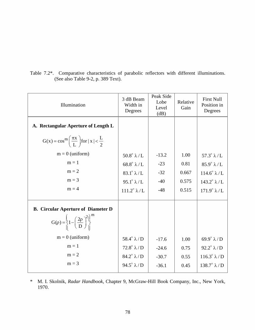
Table 7.2*. Comparative characteristics of parabolic reflectors with different illuminations. (See also Table 9-2, p. 389 Text).

Illumination 3 dB Beam Width in Degrees

Peak Side Lobe Level (dB)

Relative Gain

First Null Position in

Degrees

A. Rectangular Aperture of Length L

m x LG(x) cos for | x |

L 2π = <

m = 0 (uniform)

m = 1 m = 2

m = 3

m = 4

50.8 / Lλ

68.8 / Lλ

83.1 / Lλ

95.1 / Lλ

111.2 / Lλ

-13.2

-23

-32

-40

-48

1.00

0.81

0.667

0.575

0.515

57.3 / Lλ

85.9 / Lλ

114.6 / Lλ

143.2 / Lλ

171.9 / Lλ

B. Circular Aperture of Diameter D

m22G( ) 1D

ρ ρ = −

m = 0 (uniform)

m = 1 m = 2

m = 3

58.4 / Dλ

72.8 / Dλ

84.2 / Dλ

94.5 / Dλ

-17.6

-24.6

-30.7

-36.1

1.00

0.75

0.55

0.45

69.9 / Dλ

92.2 / Dλ

116.3 / Dλ

138.7 / Dλ

* M. I. Skolnik, Radar Handbook, Chapter 9, McGraw-Hill Book Company, Inc., New York,

1970.