Spice training network EU

ANR cattel

EARTHQUAKE DYNAMICS and

the PREDICTION of STRONG GROUND MOTION

Raoul MadariagaLaboratoire de Géologie

Ecole Normale SupérieureParis

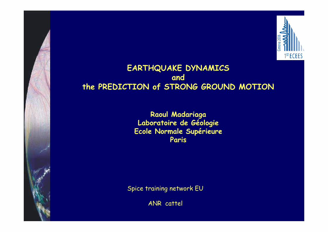
.BB Seismic waves

Hifi Seismicwaves

Different scales in earthquake dynamics

Macroscale

Mesoscale

MicroscaleSteady state mechanicsvr

(< 0.3 Hz λ> 5 km)

(>0.5 Hz λ<2 km)

(non-radiative)(λ< 100 m)

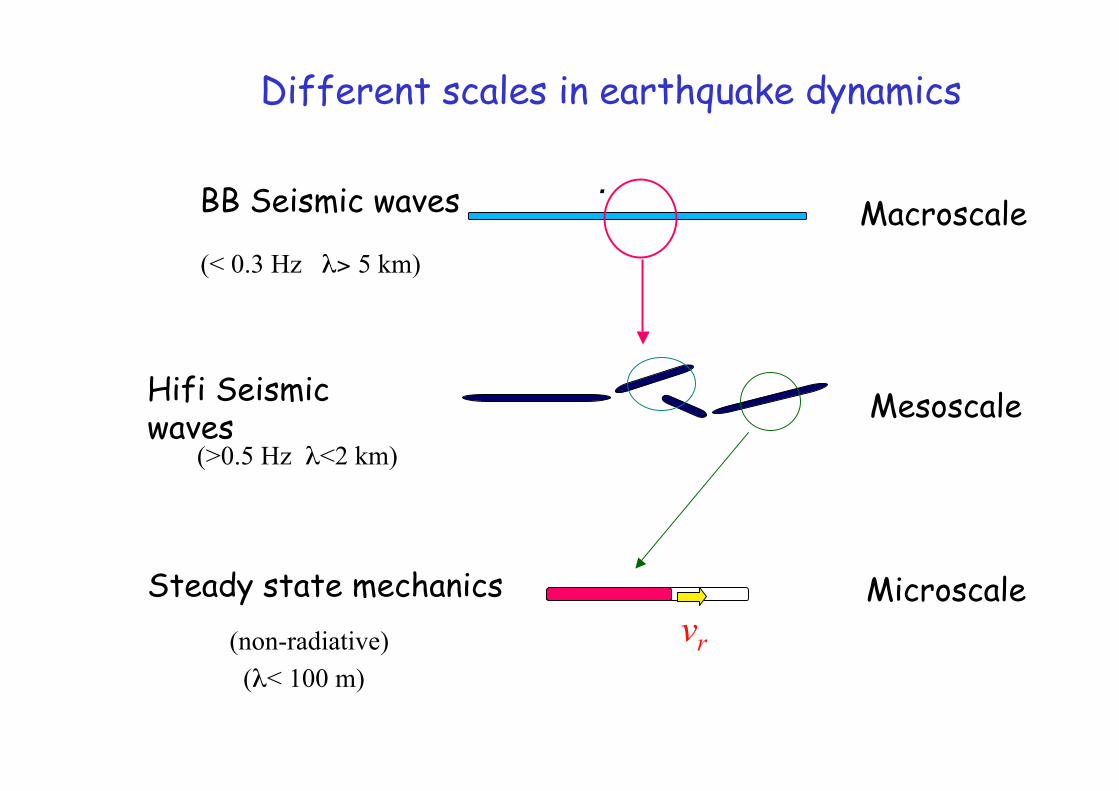
Kinematic modeling

1. Elastic model + attenuation

2.. Dislocation model

3.. Modeling program (and, of course a BIG computer)

4.. Seismic data

Slip model

Rupture process

Parkfield 2004

(after Liu et al 2006)

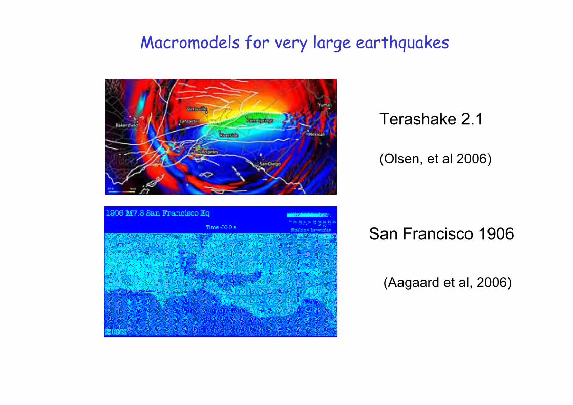
Macromodels for very large earthquakes

Terashake 2.1

(Olsen, et al 2006)

San Francisco 1906

(Aagaard et al, 2006)

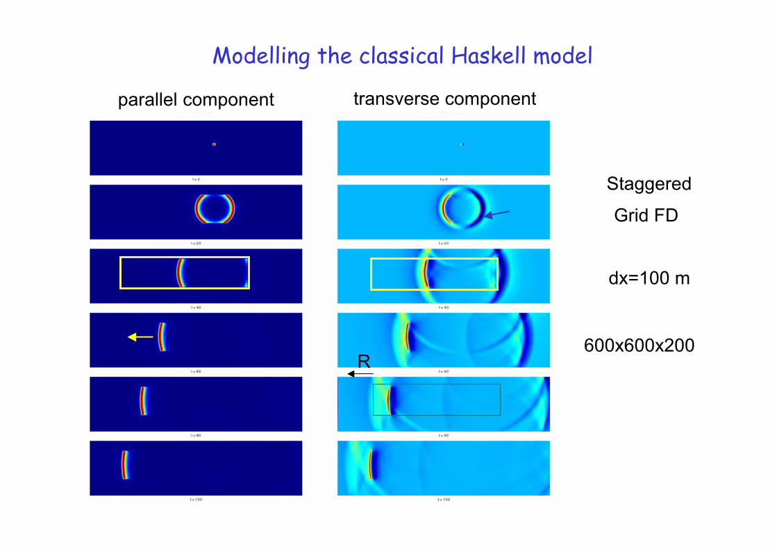
Modelling the classical Haskell model

parallel component transverse component

Staggered

Grid FD

dx=100 m

600x600x200R

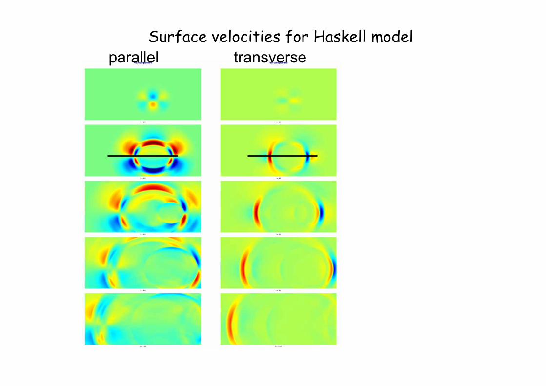
Surface velocities for Haskell modelparallel transverse

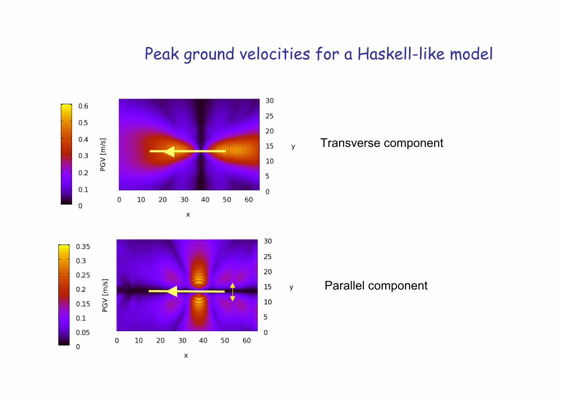
Peak ground velocities for a Haskell-like model

Transverse component

Parallel component

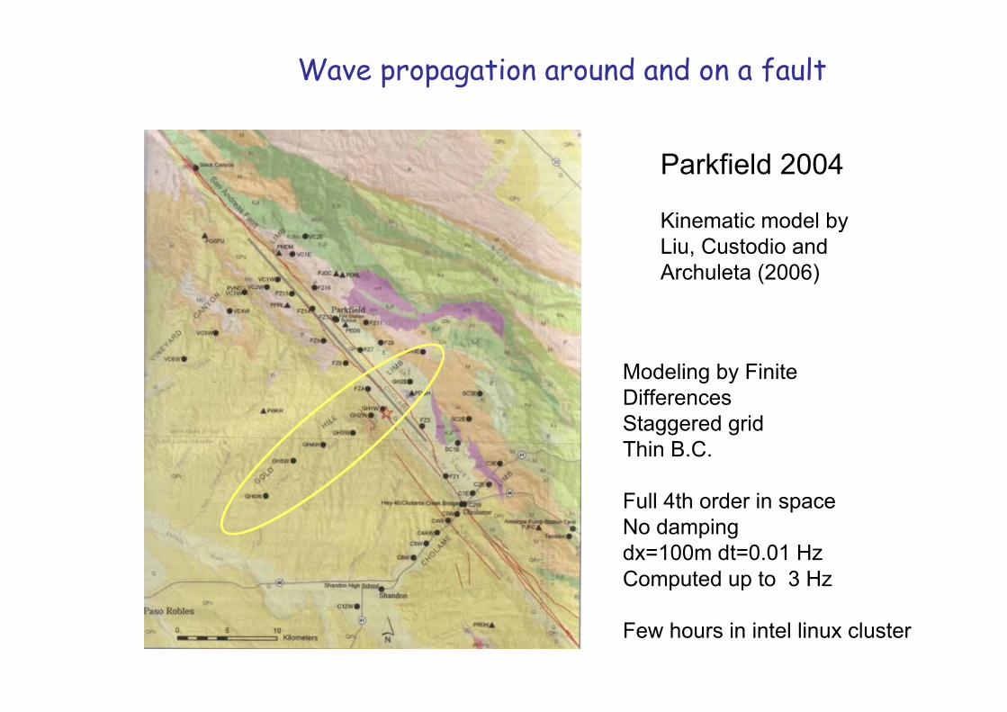
Wave propagation around and on a fault

Parkfield 2004

Kinematic model by Liu, Custodio andArchuleta (2006)

Modeling by Finite DifferencesStaggered gridThin B.C.

Full 4th order in spaceNo dampingdx=100m dt=0.01 HzComputed up to 3 Hz

Few hours in intel linux cluster

0 5 10 15 20 25-5

0

5

GH2E

Vp (cm/sec)

Observed

Synthetic

0 5 10 15 20 25-2

0

2

Vn (cm/sec)

0 5 10 15 20 25-2

0

2

Vz (cm/sec)

0 5 10 15 20 25-5

0

5

GH3E

0 5 10 15 20 25-2

0

2

0 5 10 15 20 25-1

0

1

0 5 10 15 20 25-5

0

5

GH1W

0 5 10 15 20 25-5

0

5

0 5 10 15 20 25-2

0

2

0 5 10 15 20 25-10

0

10

GH2W

0 5 10 15 20 25-5

0

5

0 5 10 15 20 25-2

0

2

0 5 10 15 20 25-10

0

10

GH3W

0 5 10 15 20 25-2

0

2

0 5 10 15 20 25-2

0

2

0 5 10 15 20 25-5

0

5

GH4W

0 5 10 15 20 25-5

0

5

0 5 10 15 20 25-2

0

2

0 5 10 15 20 25-5

0

5

GH5W

0 5 10 15 20 25-5

0

5

0 5 10 15 20 25-2

0

2

0 5 10 15 20 25-5

0

5

GH6W

time (sec)

0 5 10 15 20 25-1

0

1

time (sec)

0 5 10 15 20 25-2

0

2

time (sec)

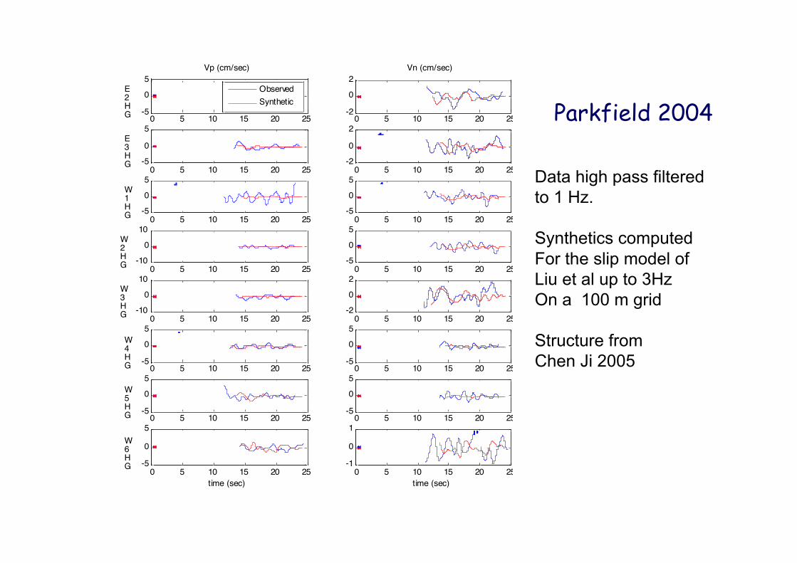
Parkfield 2004

Data high pass filtered to 1 Hz.

Synthetics computed For the slip model ofLiu et al up to 3HzOn a 100 m grid

Structure from Chen Ji 2005

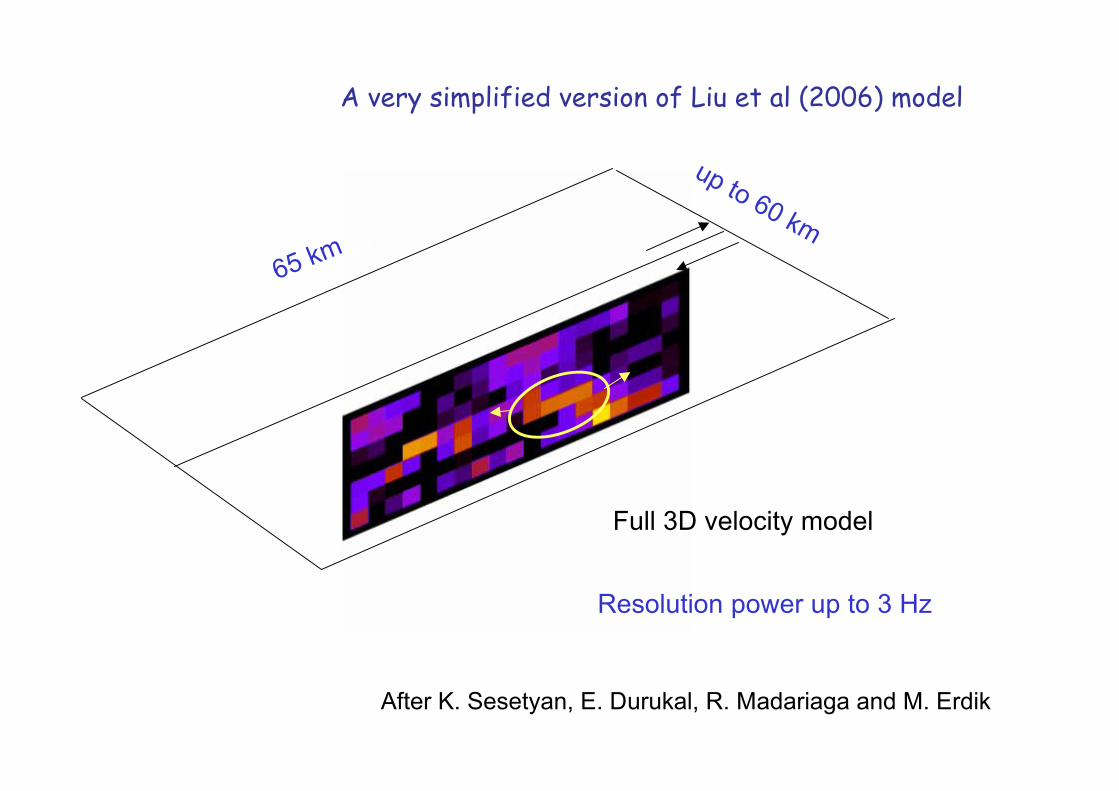
A very simplified version of Liu et al (2006) model

After K. Sesetyan, E. Durukal, R. Madariaga and M. Erdik

Full 3D velocity model

65 km65 km

up to 60 km

Resolution power up to 3 Hz

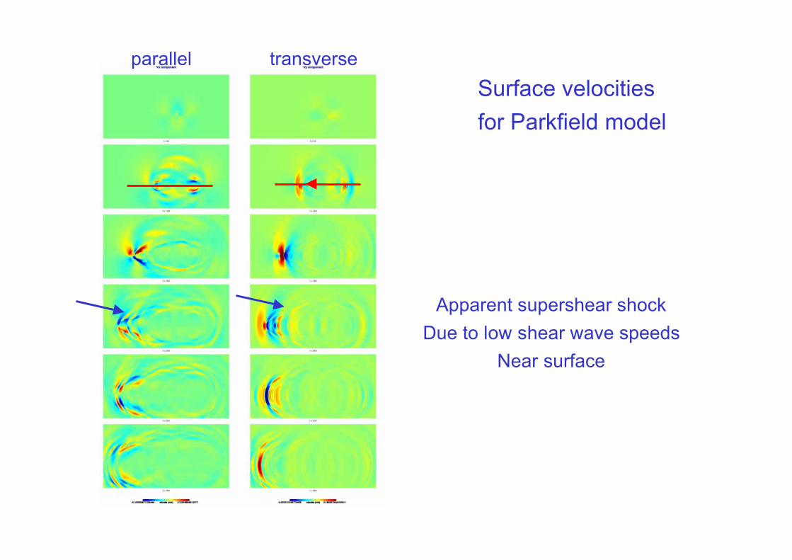
Surface velocities for Parkfield model

parallel transverse

Apparent supershear shockDue to low shear wave speeds

Near surface

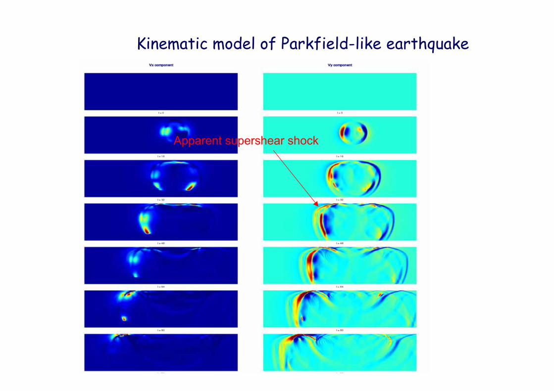
Kinematic model of Parkfield-like earthquake

Apparent supershear shock

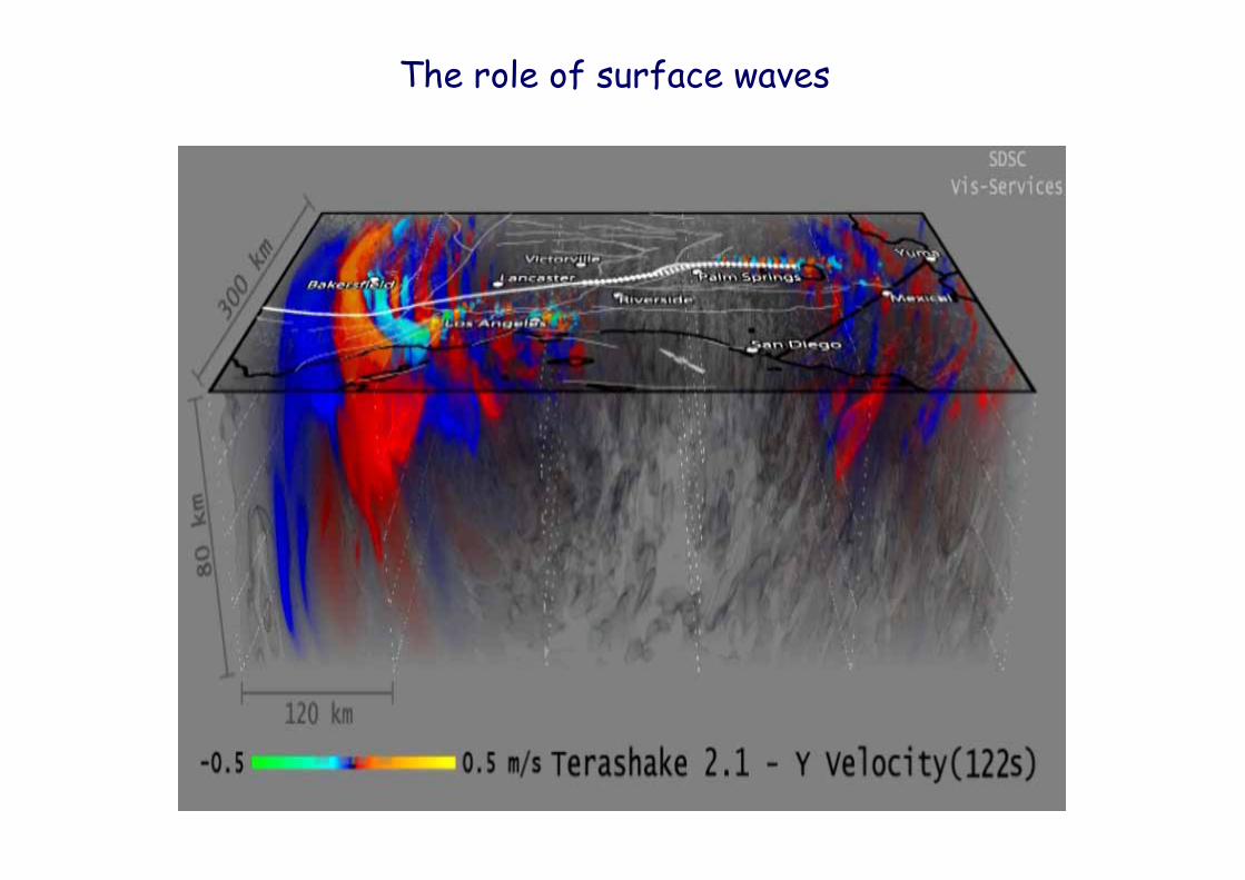
The role of surface waves

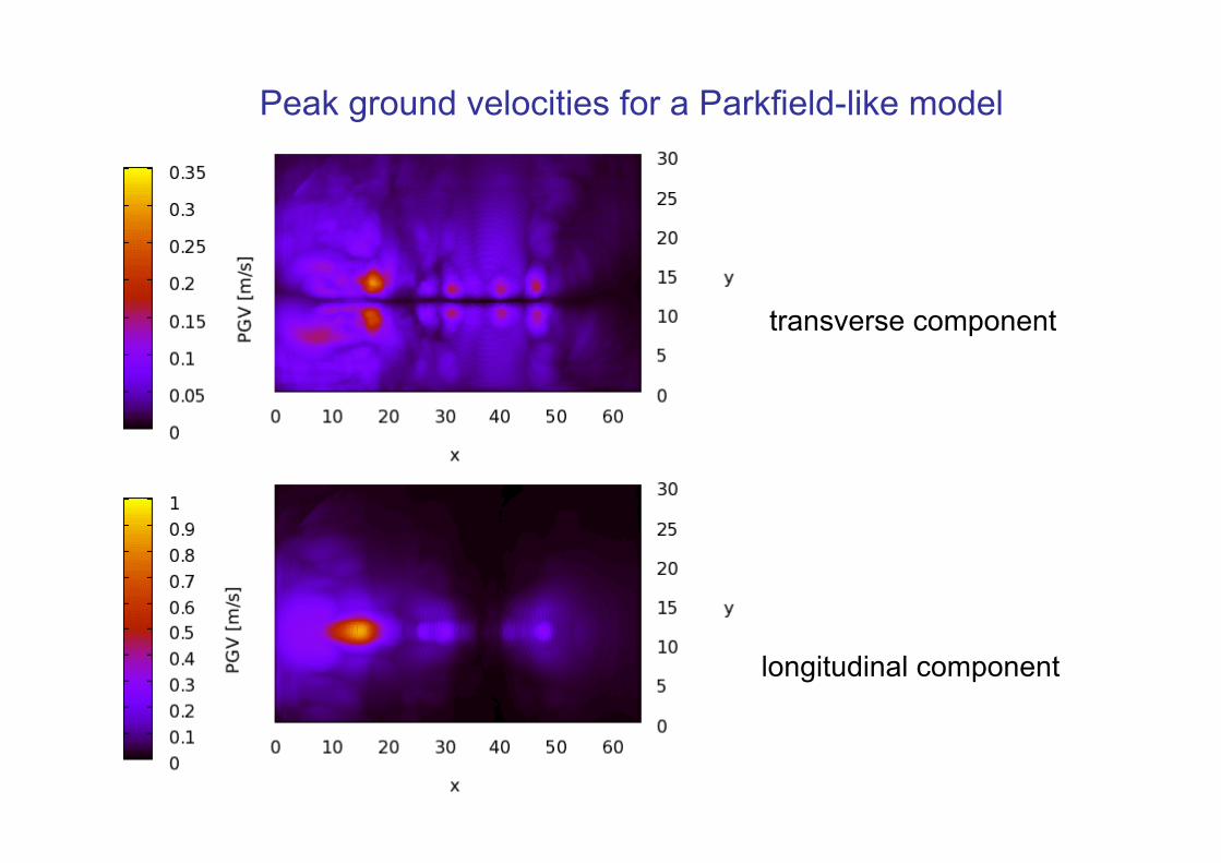
Peak ground velocities for a Parkfield-like model

transverse component

longitudinal component

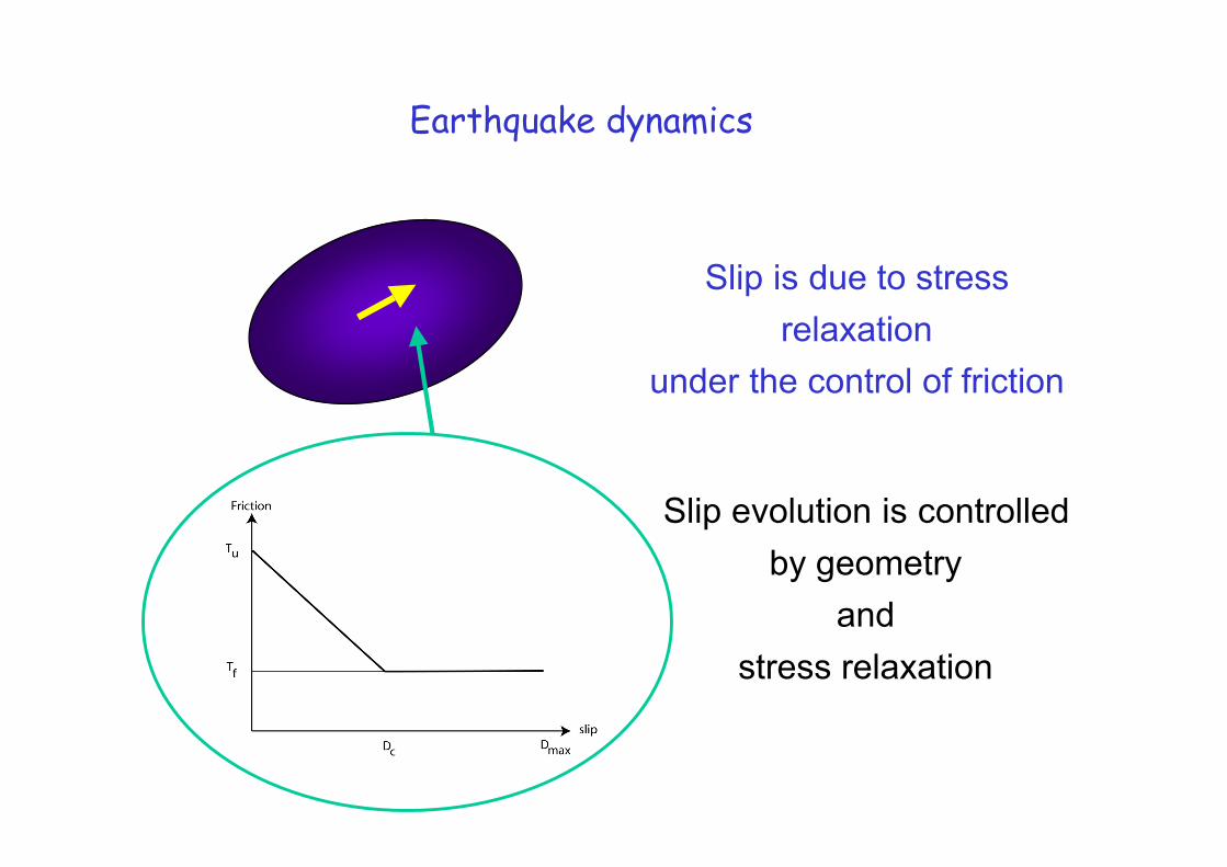
Earthquake dynamics

Slip is due to stressrelaxation

under the control of friction

Slip evolution is controlledby geometry

andstress relaxation

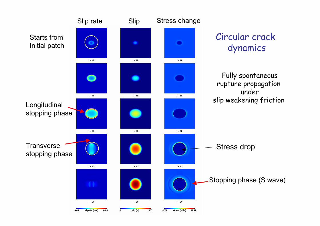
Circular crack dynamics

Starts fromInitial patch

Longitudinal stopping phase

Transversestopping phase

Stopping phase (S wave)

Slip rate Slip Stress change

Fully spontaneousrupture propagation

underslip weakening friction

Stress drop

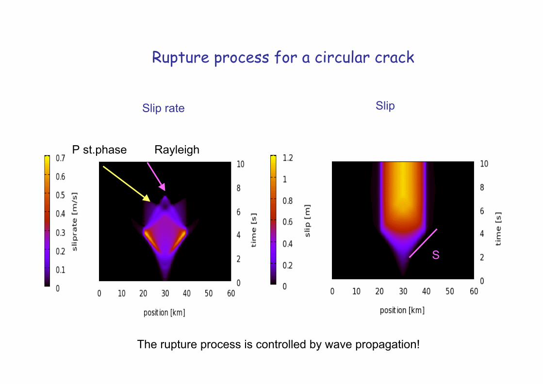
P st.phase Rayleigh

S

Slip rate Slip

Rupture process for a circular crack

The rupture process is controlled by wave propagation!

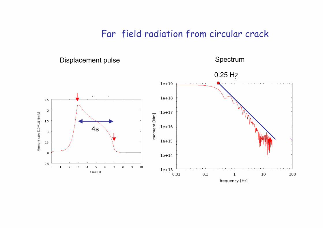
Far field radiation from circular crack

SpectrumDisplacement pulse

4s

0.25 Hz

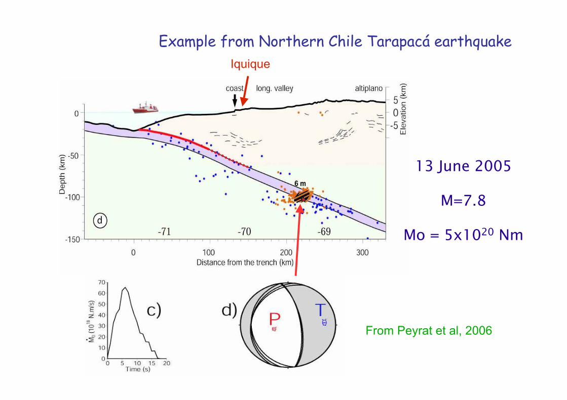
Example from Northern Chile Tarapacá earthquakeIquique

From Peyrat et al, 2006

13 June 2005

M=7.8

Mo = 5x1020 Nm

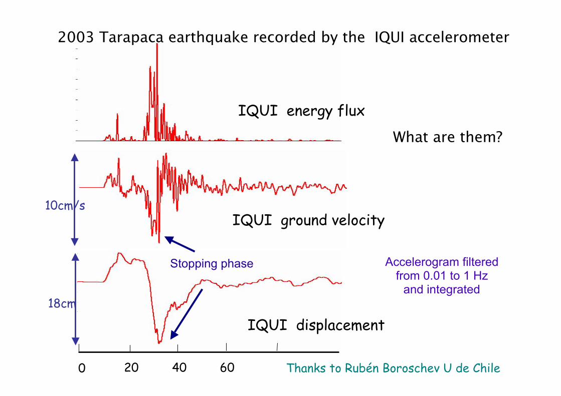
2003 Tarapaca earthquake recorded by the IQUI accelerometer

Thanks to Rubén Boroschev U de Chile

IQUI displacement

IQUI ground velocity

IQUI energy flux

What are them?

Accelerogram filteredfrom 0.01 to 1 Hz

and integrated

Stopping phase

0 4020

10cm/s

18cm

60

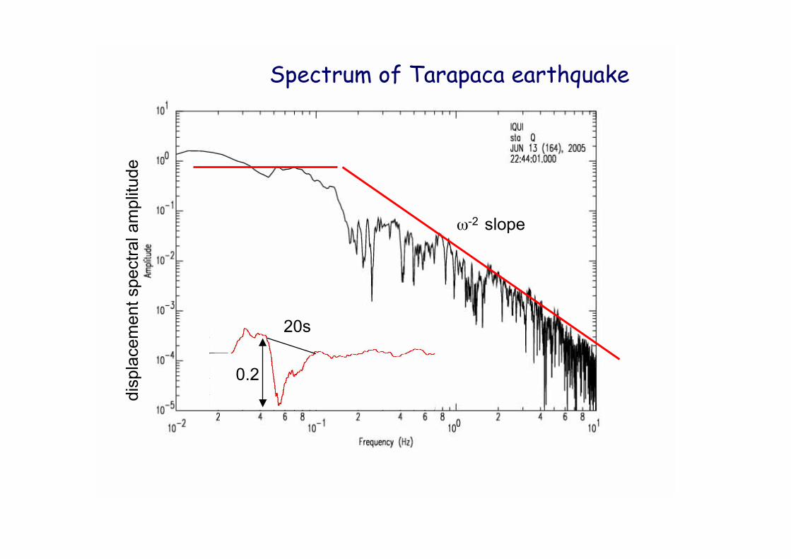
Spectrum of Tarapaca earthquake

disp

lace

men

t spe

ctra

l am

plitu

de

ω-2 slope

20s

0.2

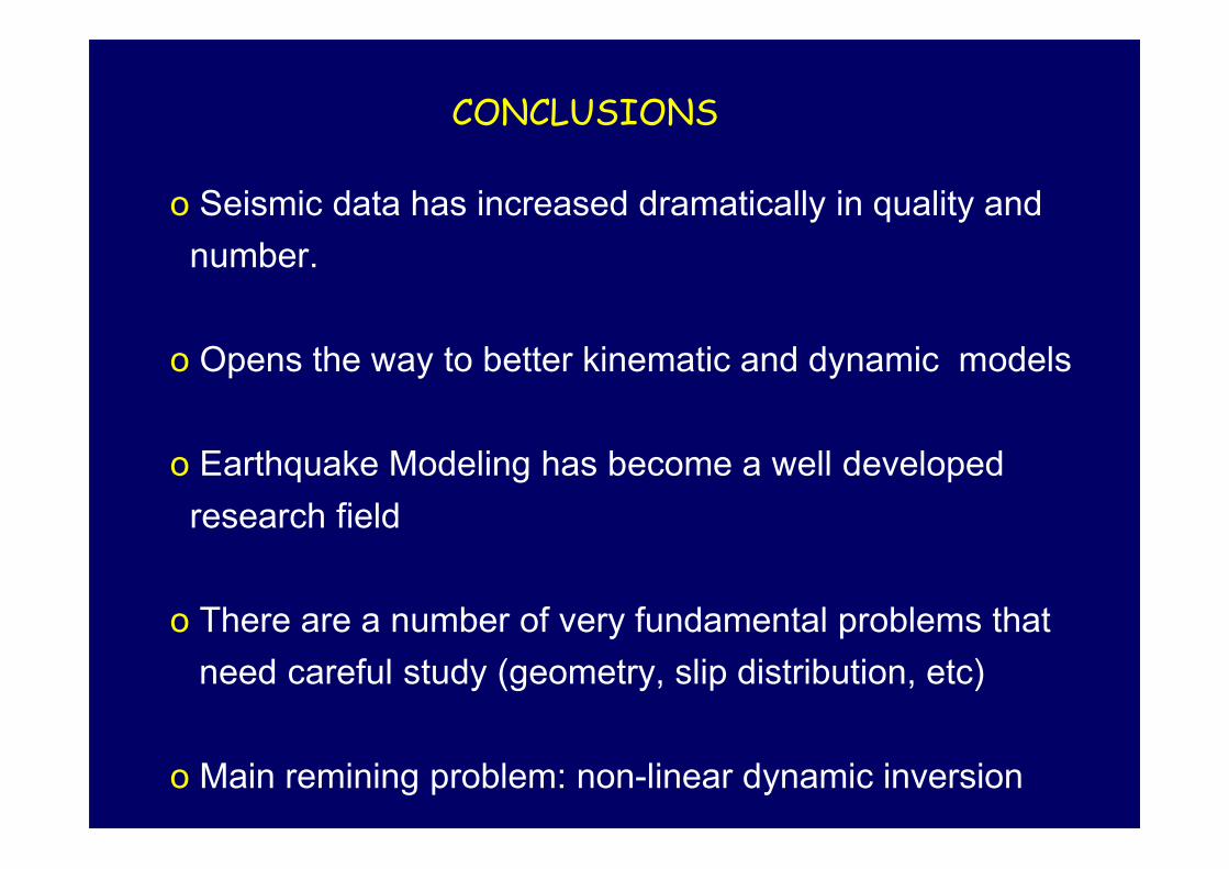
o Seismic data has increased dramatically in quality and number.

o Opens the way to better kinematic and dynamic models

o Earthquake Modeling has become a well developed research field

o There are a number of very fundamental problems that need careful study (geometry, slip distribution, etc)

o Main remining problem: non-linear dynamic inversion

CONCLUSIONS

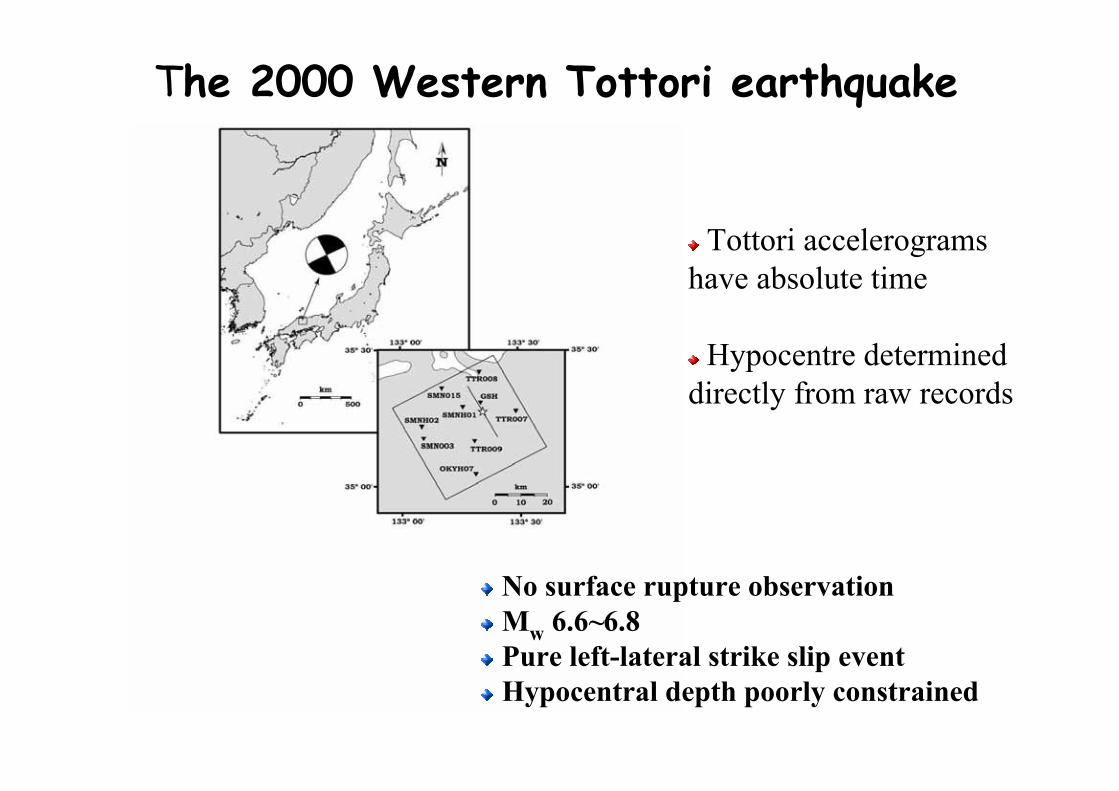
No surface rupture observationMw 6.6~6.8Pure left-lateral strike slip eventHypocentral depth poorly constrained

Tottori accelerogramshave absolute time

Hypocentre determineddirectly from raw records

The 2000 Western Tottori earthquake

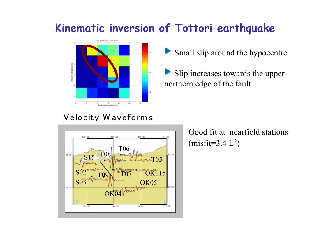
Kinematic inversion of Tottori earthquake

Small slip around the hypocentre

Slip increases towards the uppernorthern edge of the fault

Velocity W aveform s

EW component

T05

S02 OK015T07OK05

OK04

S15

S03

T06T08

T09

Good fit at nearfield stations(misfit=3.4 L2)

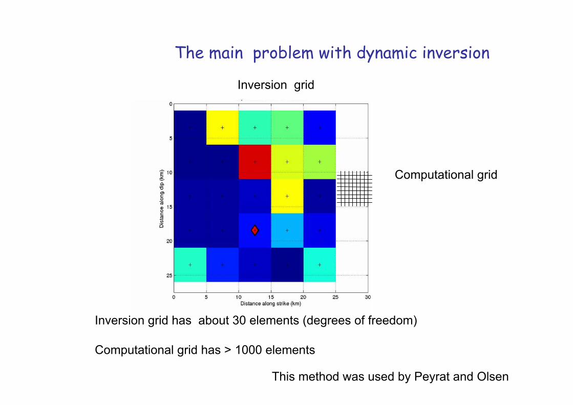
Computational grid

Inversion grid

The main problem with dynamic inversion

Inversion grid has about 30 elements (degrees of freedom)

Computational grid has > 1000 elements

This method was used by Peyrat and Olsen

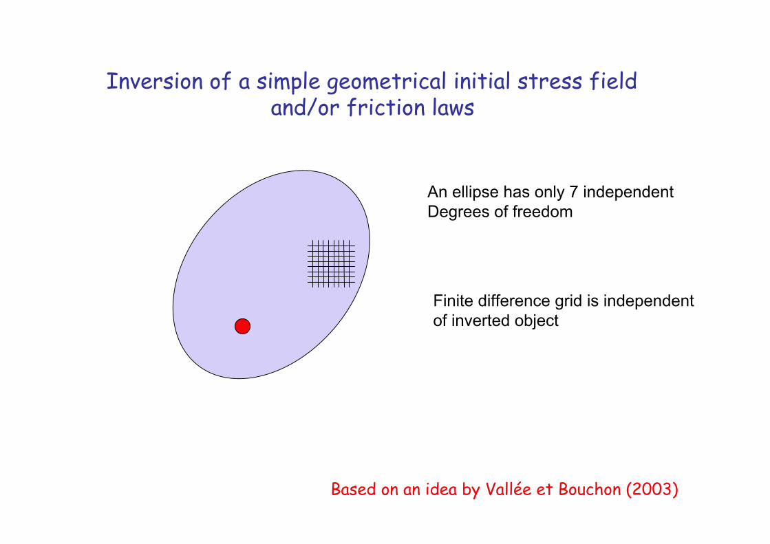
Inversion of a simple geometrical initial stress field and/or friction laws

Based on an idea by Vallée et Bouchon (2003)

An ellipse has only 7 independentDegrees of freedom

Finite difference grid is independentof inverted object

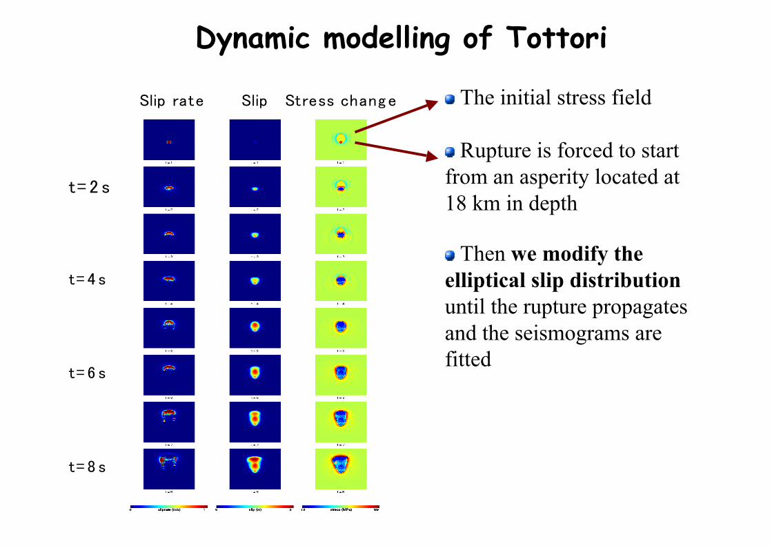
The initial stress field

Rupture is forced to startfrom an asperity located at18 km in depth

Then we modify theelliptical slip distributionuntil the rupture propagatesand the seismograms arefitted

Slip rate Slip Stress chang e

Dynamic modelling of Tottori

t= 2 s

t= 4 s

t= 6 s

t= 8 s

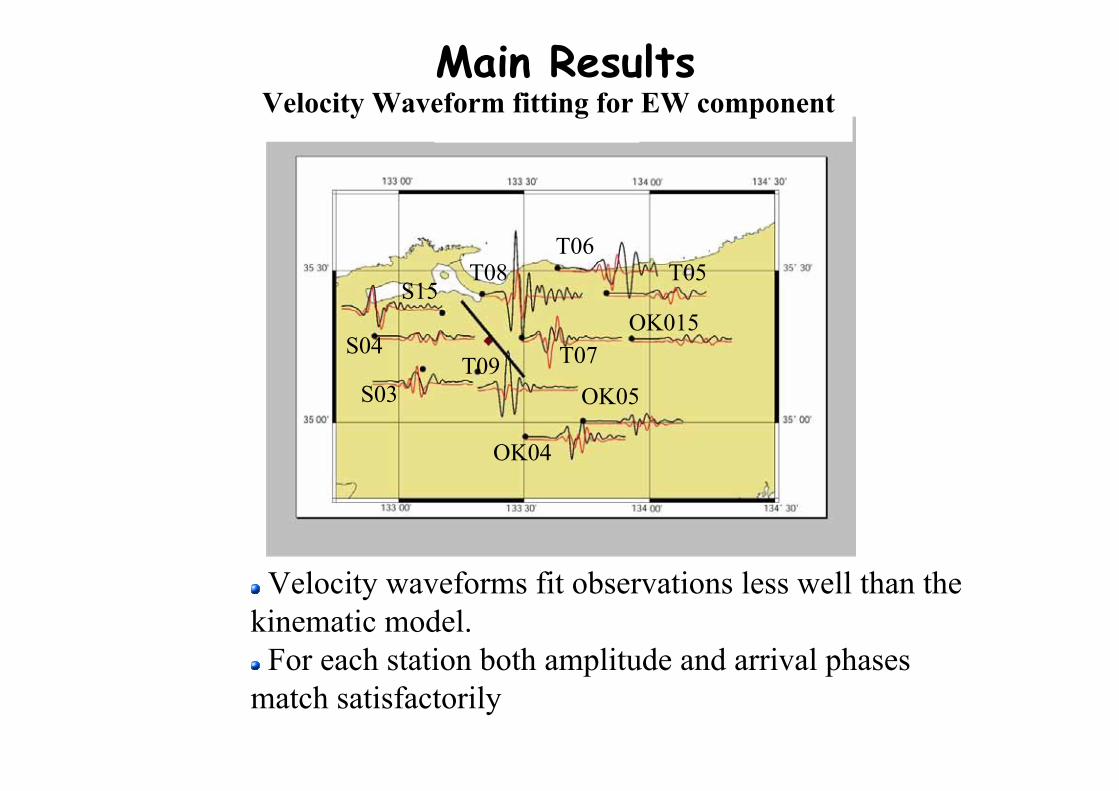
Main Results

Velocity waveforms fit observations less well than thekinematic model. For each station both amplitude and arrival phases

match satisfactorily

T05

S04OK015

T07

OK05

OK04

S15

S03

T06T08

T09

Velocity Waveform fitting for EW component

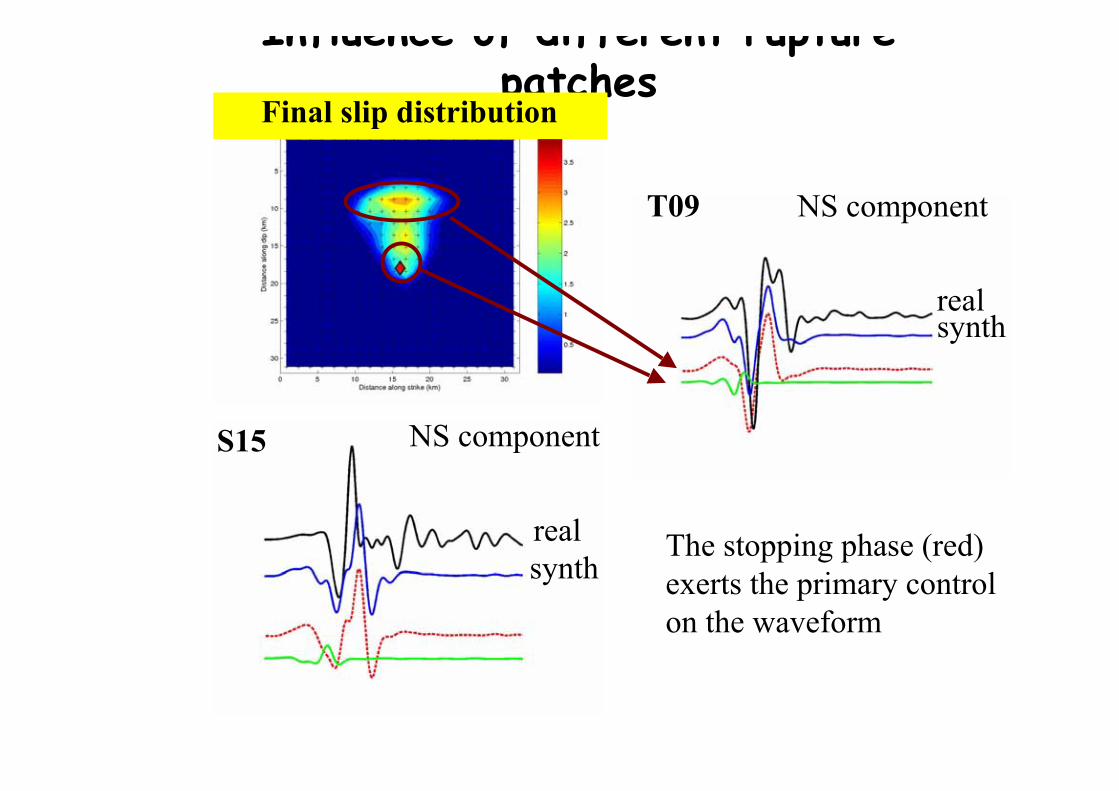
Influence of different rupturepatches

S15

T09

Final slip distribution

NS component

NS component

The stopping phase (red)exerts the primary controlon the waveform

realsynth

realsynth

OutlookTwo approaches to study the propagation of the Tottori earthquake:

The non linear kinematic inversion gives a very good wavefitscontrolled by a diagonal stopping phase.

The dynamic rupture inversion allows to fit very well bothamplitude and arrival phases. The horizontal stopping phasecontrols the waveforms.

A dynamic inversion with a slip distribution controlled by 2elliptical patches is in progress.

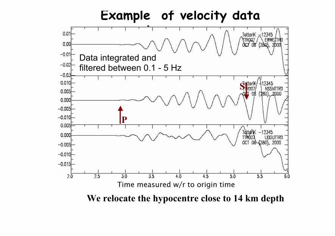
Example of velocity dataprocessing

Time measured w/r to origin time

P

S

Data integrated and filtered between 0.1 - 5 Hz

We relocate the hypocentre close to 14 km depth