Dynare & Bayesian Estimation

Wouter J. Den HaanLondon School of Economics

c© 2011 by Wouter J. Den Haan

August 19, 2011

Overview Basics MCMC Generated output Shocks versus model Trends The big issues

Overview of the program

• Calculate likelihood, L(YT|Ψ)• Calculate posterior, P(Ψ|YT) ∝ L(YT|Ψ)P(Ψ)• Calculate mode• Calculate preliminary info about posterior

• using quick and dirty assumption of normality

• Use MCMC to• trace the shape of P(Ψ|YT)• calculate things like confidence intervals

• Plot graphs

Overview Basics MCMC Generated output Shocks versus model Trends The big issues

Calculate Likelihood as function of psi

• Given Ψ, get first-order approximation of the model• Write the system in state-space notation• Use the Kalman filter to back out

yt = yt − E[yt|Yt−1, x1

]and Σy,t

• yt vector with ny observed values• E

[yt|Yt−1, x1

]prediction according to Kalman filter

• yt : prediction error• yt : function of all the shocks in the model

• Linearity =⇒• yt ∼ N(0, Σy,t)• likelihood of sequence can be calculated

Overview Basics MCMC Generated output Shocks versus model Trends The big issues

Calculate posterior & mode

P(Ψ|YT) ∝ L(YT|Ψ)P(Ψ)

• P(Ψ|YT) is a complex function• But its value can be calculated easily for given Ψ• =⇒ value of Ψ that attains the max can be calculated using anoptimization routine(in practice, max of P(Ψ|YT) much easier to find than max ofL(YT|Ψ) because P (Ψ) makes problem better behaved)

Overview Basics MCMC Generated output Shocks versus model Trends The big issues

Information about posterior using MCMC

• But we want to calculate objects like

E [g(Ψ)] =∫

g(Ψ)P(Ψ|YT)dΨ∫P(Ψ|YT)dΨ

• Examples, mean, standard errors, confidence intervalsthese are all integrals

Overview Basics MCMC Generated output Shocks versus model Trends The big issues

Idea behing MCMC

• Problem: We cannot draw numbers directly from P(Ψ|YT)

• Solution: Generate a sequence for ψ such that its distributionis equal to P(Ψ|YT)

Implementing MCMC is not trivial!!!

Overview Basics MCMC Generated output Shocks versus model Trends The big issues

Part I:initialization

// dynareestimate.mod

var lc, lk, lz, ly;varexo e;parameters beta, rho, alpha, nu, delta;

Overview Basics MCMC Generated output Shocks versus model Trends The big issues

Part II:set values for parameters that arenot estimated

alpha = 0.36;rho = 0.95;beta = 0.99;nu = 1;delta = 0.025;

• Values will be ignored during estimation• So only needed if you first give Dynare commands that requireparameter values

Overview Basics MCMC Generated output Shocks versus model Trends The big issues

Part III: model

model;

exp(-nu*lc)=beta*(exp(-nu*lc(+1)))*(exp(lz(+1))*alpha*exp((alpha-1)*lk)+1-delta);

exp(lc)+exp(lk)=exp(lz+alpha*lk(-1))+(1-delta)*exp(lk(-1));

lz = rho*lz(-1)+e;

end;

Overview Basics MCMC Generated output Shocks versus model Trends The big issues

Part IV (optional): analyze model solution& properties for specified parameter values

steady;Stoch_simul(order=1,nocorr,nomoments,IRF=12);

• This requires having given numerical values for all parameters

Overview Basics MCMC Generated output Shocks versus model Trends The big issues

Part V: define priors

estimated_params;alpha, inv_gamma_pdf, 0.007, inf;end;

• more alternatives given below

Overview Basics MCMC Generated output Shocks versus model Trends The big issues

Part V: initialize estimation

Tell dynare what the observables are

varobs lk;

Overview Basics MCMC Generated output Shocks versus model Trends The big issues

Part V: initialize estimation

Give initial values for steady state

initval;lc = -1.02;lk = -1.61;lz = 0;end;

Overview Basics MCMC Generated output Shocks versus model Trends The big issues

Calculate steady state

Steady state must be calculated for many different values of Ψ !!!

• Linearize the system yourself• then easy to solve for steady state

• Give the exact solution of steady state as initial values• Provide program to calculate the steady state yourself

Overview Basics MCMC Generated output Shocks versus model Trends The big issues

Calculate steady state yourself

• If your *.mod file is called xxx.mod then write a filexxx_steadystate.m

• dynare checks whether a file with this name exists and will use it• sequence of output should correspond with sequence given invar list

Overview Basics MCMC Generated output Shocks versus model Trends The big issues

Calculate steady state yourselffunction [ys,check] = modela_steadystate(ys,exe)global M_

beta = M_.params(1);rho = M_.params(2);alpha = M_.params(3);nu = M_.params(4);delta = M_.params(5);sig = M_.params(6);check = 0;

z = 1;k = ((1-beta*(1-delta))/(alpha*beta))^(1/(alpha-1));c = k^alpha-delta*k;

ys =[ c; k; z ];

Overview Basics MCMC Generated output Shocks versus model Trends The big issues

How to create this file?

In your *.mod file include:

steady_state_model;z = 1;k = ((1-beta*(1-delta))/(alpha*beta))^(1/(alpha-1));c = k^alpha-delta*k;end;

Overview Basics MCMC Generated output Shocks versus model Trends The big issues

When it has been created?

• Now that the file has been created you can do more things:• e.g. solve for some analytically and some numerically

Overview Basics MCMC Generated output Shocks versus model Trends The big issues

Part VI: Estimation

Actual estimation command with some of the possible options

estimation(datafile=kdata,mh_nblocks=5,mh_replic=10000,mh_jscale=3,mh_init_scale=12) lk;

• lk: (optional) name of the endogenous variables (e.g. if youwant to plot Bayesian IRFs)

• datafile: contains observables• kdata.mat or kdata.m or kdata.xls

• nobs: number of observations used (default all)• first_obs: first observation (default is first)

Overview Basics MCMC Generated output Shocks versus model Trends The big issues

MCMC options

• mh_replic: number of observations in each MCMC sequence• mh_nblocks: number of MCMC sequences• mh_jscale: variance of the jumps in Ψ in MCMC chain

• a higher value of mh_jscale =⇒ bigger steps through thedomain of Ψ & lower acceptance ratio

• acceptance ratio should be around 0.234(according to some optimality results; see below)

• mh_init_scale: variance of initial draw• important to make sure that the different MCMC sequencesstart in different points

Overview Basics MCMC Generated output Shocks versus model Trends The big issues

Part VII: Using estimated model

Acutal estimation command with some of the possible options

shock_decomposition;

• plots graphs with the observables and the partexplained by which shock.

Overview Basics MCMC Generated output Shocks versus model Trends The big issues

Priors - format

estimated_params;parameter name, prior_shape, prior_mean,prior_standarddeviation[,prior 3rd par. value, prior 4th par. value];end

the part in [] only for some priors

Overview Basics MCMC Generated output Shocks versus model Trends The big issues

Priors - examples

alpha’s prior is Normal with mean mu and standard deviation sigma:

alpha , normal_pdf,mu,sigma;

alpha’s prior is uniform over [p3,p4]:

alpha , uniform_pdf, , , p3, p4;

Note the two spaces betweeen the commas

Overview Basics MCMC Generated output Shocks versus model Trends The big issues

Priors - innovation variances

• use "stderr e" as the parameter name for the innovationvariance.

• For example,• stderr e , uniform_pdf, , , p3, p4;

Note the two empty spaces betweeen the commas

Overview Basics MCMC Generated output Shocks versus model Trends The big issues

Priors - examples

name distribution & parameters rangenormal_pdf N(µ, σ) R

gamma_pdf G2(µ, σ, p3) [p3,+∞)beta_pdf B(µ, σ, p3, p4) [p3, p4]inv_gamma_pdf IG1(µ, σ) R+

uniform_pdf U(p3, p4) [p3, p4]

Overview Basics MCMC Generated output Shocks versus model Trends The big issues

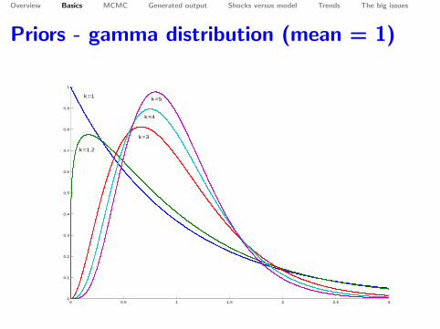
Priors - gamma distribution

P(x− p3) = (x− p3)k−1 exp (− (x− p3) /θ)

Γ (k) θk

Γ (k) = (k− 1)! if k is an integer

Γ (k) =∫ ∞

0tk−1e−tdt o.w.

k : shape parameter

θ : scale parameter

µ = kθ

σ2 = kθ2

skewness = E (x− p3)3 /(E[(x− p3)

2])3/2

= 2/√

κ

mode : p3 + (k− 1)θ for k ≥ 1

Overview Basics MCMC Generated output Shocks versus model Trends The big issues

Priors - gamma distribution

• If k = 1 =⇒ mode at lower bound• If k = 1 =⇒ exponential• If k = degrees of freedom/2 en θ = 2 =⇒ Chi-squared• Gamma distribution is right-skewed

Overview Basics MCMC Generated output Shocks versus model Trends The big issues

Priors - gamma distribution (mean = 1)

0 0.5 1 1.5 2 2.5 30

0.1

0.2

0.3

0.4

0.5

0.6

0.7

0.8

0.9

1

k=1.2

k=3

k=4

k=1 k=5

Overview Basics MCMC Generated output Shocks versus model Trends The big issues

Priors - inverse gamma distribution-

• If X has a gamma(k, θ) =⇒1/X has an inverse gamma distribution(κ, 1/θ)

Overview Basics MCMC Generated output Shocks versus model Trends The big issues

Priors - inverse gamma distribution

P(x) = x−k−1 θk exp (−θ/x)Γ(k)

k : shape parameter

θ : scale parameter

µ = θ/ (k− 1) for k > 1

σ2 = θ2/((k− 1)2 (k− 2)

)for k > 2

skewness = 4√(k− 2)/ (k− 3) for k > 3

mode : θ/ (k+ 1)

Overview Basics MCMC Generated output Shocks versus model Trends The big issues

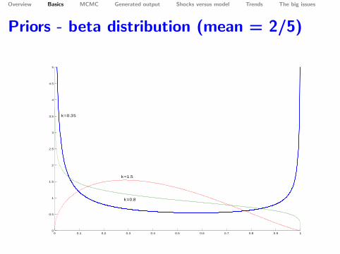
Priors - beta distribution on [0,1]

P(x) =xφ−1 (1− x)θ−1

B (φ, θ)

B(k, θ) =Γ (φ+ θ)

Γ (φ) Γ (θ)φ : shape parameter

θ : shape parameter

µ = φ/ (φ+ θ)

σ2 = φθ/((φ+ θ)2 (φ+ θ + 1)

)skewness =

2 (θ − φ)√

φ+ θ + 1(φ+ θ + 2)

√φθ

mode :φ− 1

φ+ θ − 2for φ > 1, θ > 1

Overview Basics MCMC Generated output Shocks versus model Trends The big issues

Priors - beta distribution

• If φ < 1, θ < 1 =⇒ U-shaped• If φ > 1, θ > 1 =⇒ unimodal• If φ < 1, θ ≥ 1 or φ = 1, θ > 1 =⇒ strictly decreasing

• If φ = 1, θ > 2 =⇒ strictly convex• If φ = 1, 1 < θ < 2 =⇒ strictly concave

• If φ > 1, θ ≤ 1 or φ = 1, θ < 1 =⇒ strictly increasing

• If θ = 1, φ > 2 =⇒ strictly convex• If θ = 1, 1 < φ < 2 =⇒ strictly concave

Overview Basics MCMC Generated output Shocks versus model Trends The big issues

Priors - beta distribution (mean = 2/5)

0 0.1 0.2 0.3 0.4 0.5 0.6 0.7 0.8 0.9 10

0.5

1

1.5

2

2.5

3

3.5

4

4.5

5

k=0.35

k=1.5

k=0.8

Overview Basics MCMC Generated output Shocks versus model Trends The big issues

Brooks & Gelman 1989 statistics

• MCMC: should generate sequence as if drawn from P(Ψ|YT)

• Tough to check• Minimum requirement is that distribution is same

• for different parts of the same sequence• across sequences (if you have more than one)

Overview Basics MCMC Generated output Shocks versus model Trends The big issues

Brooks & Gelman 1989 statistics

• Ψij the ith draw (out of I) in the jth sequence (out of J)

• Ψ·j mean of jth sequence• Ψ·· mean across all available data

Overview Basics MCMC Generated output Shocks versus model Trends The big issues

Between variance

B =1

J− 1

J

∑j=1

(Ψ·j − Ψ··

)2

• B is an estimate of the variance of the mean (σ2/I)=⇒ B = BI is an estimate of the variance

Overview Basics MCMC Generated output Shocks versus model Trends The big issues

Within variance

W =1J

J

∑j=1

1I

I

∑t=1

(Ψtj − Ψ·j

)2

W =1J

J

∑j=1

1I− 1

I

∑t=1

(Ψtj − Ψ·j

)2

• W and W are estimates of the variance (averaged acrossstreams)

Overview Basics MCMC Generated output Shocks versus model Trends The big issues

What do we need?

1 Between variance should go to zerolimI−→∞B −→ 0

2 Within variance should settle downlimI−→∞W −→ constant

Overview Basics MCMC Generated output Shocks versus model Trends The big issues

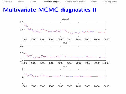
What do we need

reported by Dynare

red line : Wblue line : VAR = W+ B

We need

1 red and blue line to get close

2 red line to settle down

Overview Basics MCMC Generated output Shocks versus model Trends The big issues

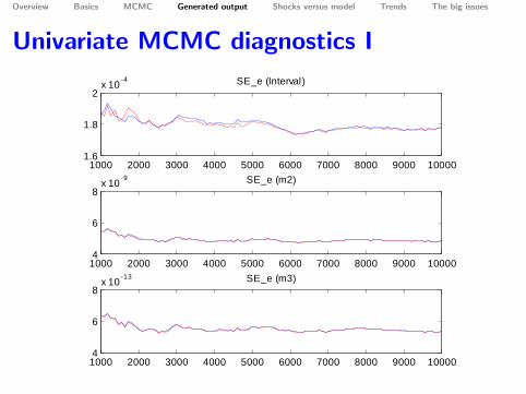
Univariate extensions

• The above can be done for any moment, not just the variance• Dynare reports three alternatives

Overview Basics MCMC Generated output Shocks versus model Trends The big issues

Multivariate extension

• For each moment of interest you can calculate the multivariateversion

• e.g. covariance matrix for the variance• these higher-dimensional objects have to be transformed intoscalar objects that can be plotted

• See: Brooks and Gilman 1989

Overview Basics MCMC Generated output Shocks versus model Trends The big issues

Acceptance rate

• The MCMC chain has to cover the whole state space• Roberts, Gelman, & Gilks (1997): optimal acceptance rate =0.234

• Great but · · ·• optimality is an asymptotic result (if dimension of Ψ −→ ∞)• optimality relies on assumption that elements of Ψ areindependent (or another assumption replacing this one).

Overview Basics MCMC Generated output Shocks versus model Trends The big issues

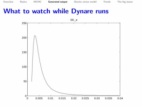
What to watch while Dynare runs

Plots here from two examples

1 As good as it gets: estimate only 1 parameter

2 Estimate all parameters

• Both cases 5,000 observations• No misspecification of the model

• i.e., artificial data

Overview Basics MCMC Generated output Shocks versus model Trends The big issues

What to watch while Dynare runs

0 0.005 0.01 0.015 0.02 0.025 0.03 0.035 0.040

50

100

150

200

250SE_e

Overview Basics MCMC Generated output Shocks versus model Trends The big issues

What to watch while Dynare runs

• When Dynare gets to the MCMC part a window opens tellingyou

• in which MCMC run you are• which fraction has been completed• most importantly the acceptance rate

• The acceptance rate should be "around" 0.234• a relatively low acceptance rate makes it more likely that theMCMC travels through the whole domain of Ψ

• acceptance rate too high =⇒ increase mh_jscale

Overview Basics MCMC Generated output Shocks versus model Trends The big issues

Tables

• RESULTS FROM POSTERIOR MAXIMIZATION

• generated before MCMC part• most important is the mode, the other stuff is based onnormality assumptions which are typically not valid

• ESTIMATION RESULTS (based on MCMC)

Overview Basics MCMC Generated output Shocks versus model Trends The big issues

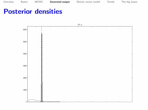
Graphs

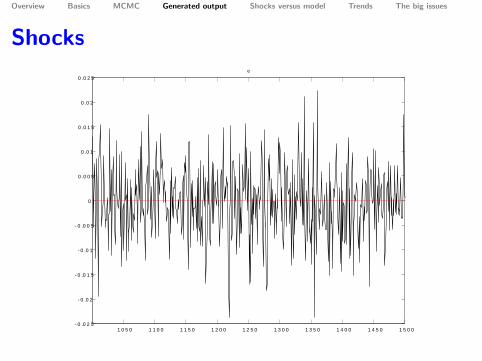
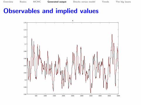
• Prior• MCMC diagnostics (see below)• Prior & posterior densities• Shocks implied at the mode• Observable and corresponding implied value

Overview Basics MCMC Generated output Shocks versus model Trends The big issues

Output for first example

• Estimate only 1 parameter, standard deviation innovation• correctly specified (neoclassical growth) model• 5,000 observations

Overview Basics MCMC Generated output Shocks versus model Trends The big issues

Univariate MCMC diagnostics I

1000 2000 3000 4000 5000 6000 7000 8000 9000 100001.6

1.8

2x 10 ­4 SE_e (Interval)

1000 2000 3000 4000 5000 6000 7000 8000 9000 100004

6

8x 10 ­9 SE_e (m2)

1000 2000 3000 4000 5000 6000 7000 8000 9000 100004

6

8x 10 ­13 SE_e (m3)

Overview Basics MCMC Generated output Shocks versus model Trends The big issues

Multivariate MCMC diagnostics II

1000 2000 3000 4000 5000 6000 7000 8000 9000 10000

1.4

1.6Interval

1000 2000 3000 4000 5000 6000 7000 8000 9000 100000.4

0.6

0.8m2

1000 2000 3000 4000 5000 6000 7000 8000 9000 100000

1

2m3

Overview Basics MCMC Generated output Shocks versus model Trends The big issues

Posterior densities

0.005 0.01 0.015 0.02 0.025 0.03 0.0350

1000

2000

3000

4000

5000

6000

SE_e

Overview Basics MCMC Generated output Shocks versus model Trends The big issues

Shocks

1 0 5 0 1 1 0 0 1 1 5 0 1 2 0 0 1 2 5 0 1 3 0 0 1 3 5 0 1 4 0 0 1 4 5 0 1 5 0 0­ 0 .0 2 5

­ 0 .0 2

­ 0 .0 1 5

­ 0 .0 1

­ 0 .0 0 5

0

0 .0 0 5

0 .0 1

0 .0 1 5

0 .0 2

0 .0 2 5e

Overview Basics MCMC Generated output Shocks versus model Trends The big issues

Observables and implied values

500 1000 1500 2000 2500 3000 3500 4000 4500 50003.56

3.58

3.6

3.62

3.64

3.66

3.68

3.7

3.72

3.74

3.76lk

Overview Basics MCMC Generated output Shocks versus model Trends The big issues

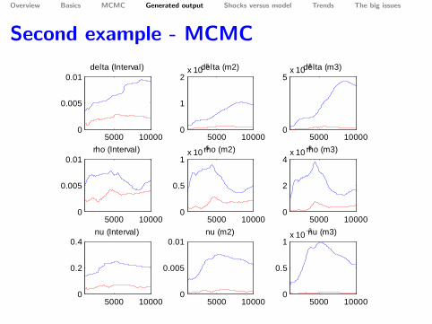
Output for second example

• Estimate all parameters• correctly specified (neoclassical growth) model• 5,000 observations

Overview Basics MCMC Generated output Shocks versus model Trends The big issues

Second example - MCMC

5000 100000

0.005

0.01delta (Interval)

5000 100000

1

2x 10 ­5delta (m2)

5000 100000

5x 10 ­8delta (m3)

5000 100000

0.005

0.01rho (Interval)

5000 100000

0.5

1x 10 ­5rho (m2)

5000 100000

2

4x 10 ­8rho (m3)

5000 100000

0.2

0.4nu (Interval)

5000 100000

0.005

0.01nu (m2)

5000 100000

0.5

1x 10 ­3nu (m3)

Overview Basics MCMC Generated output Shocks versus model Trends The big issues

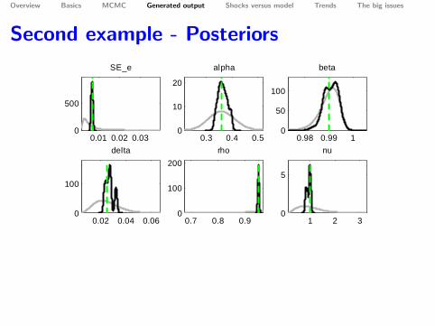
Second example - Posteriors

0.01 0.02 0.030

500

SE_e

0.3 0.4 0.50

10

20

alpha

0.98 0.99 10

50

100

beta

0.02 0.04 0.060

100

delta

0.7 0.8 0.90

100

200rho

1 2 30

5

nu

Overview Basics MCMC Generated output Shocks versus model Trends The big issues

How to make the MCMC pics look better?

Problem:

• Parameters not well identified, possibly because the dynamicsof the model are too simple; capital is not much more than ascaled up version of productivity

• More data doesn’t seem to help

Overview Basics MCMC Generated output Shocks versus model Trends The big issues

Are dynamics caused by model or shocks?

• What explains the data, the shocks or the model?• How much propagation does the model really have?• Two examples:

• Standard RBC• Christiano, Motto, Rostagno

Overview Basics MCMC Generated output Shocks versus model Trends The big issues

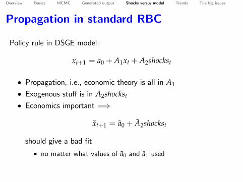
Propagation in standard RBC

Policy rule in DSGE model:

xt+1 = a0 +A1xt +A2shockst

• Propagation, i.e., economic theory is all in A1

• Exogenous stuff is in A2shockst

• Economics important =⇒

xt+1 = a0 + A2shockst

should give a bad fit

• no matter what values of a0 and a1 used

Overview Basics MCMC Generated output Shocks versus model Trends The big issues

Check importance of economics in yourmodel

• Let

arg mina0,a1

T

∑t=2

(xt+1 − a0 − A2shockst

)2

• plot {xt+1, xt+1}

Overview Basics MCMC Generated output Shocks versus model Trends The big issues

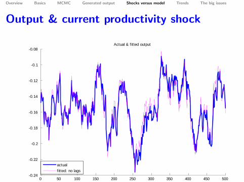
Example

• Propagation in standard growth model• Why would the endogenous variables not follow driving process

1 for 1?

Overview Basics MCMC Generated output Shocks versus model Trends The big issues

Output & current productivity shock

0 50 100 150 200 250 300 350 400 450 500­0.24

­0.22

­0.2

­0.18

­0.16

­0.14

­0.12

­0.1

­0.08Actual & fitted output

actualfitted: no lags

Overview Basics MCMC Generated output Shocks versus model Trends The big issues

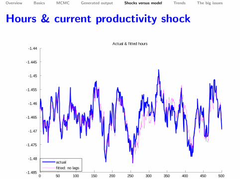
Hours & current productivity shock

0 50 100 150 200 250 300 350 400 450 500­1.485

­1.48

­1.475

­1.47

­1.465

­1.46

­1.455

­1.45

­1.445

­1.44Actual & fitted hours

actualfitted: no lags

Overview Basics MCMC Generated output Shocks versus model Trends The big issues

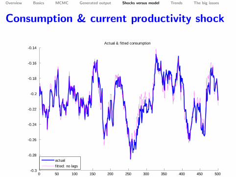
Consumption & current productivity shock

0 50 100 150 200 250 300 350 400 450 500­0.3

­0.28

­0.26

­0.24

­0.22

­0.2

­0.18

­0.16

­0.14Actual & fitted consumption

actualfitted: no lags

Overview Basics MCMC Generated output Shocks versus model Trends The big issues

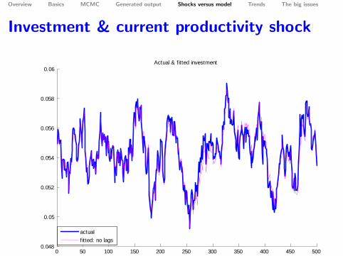
Investment & current productivity shock

0 50 100 150 200 250 300 350 400 450 5000.048

0.05

0.052

0.054

0.056

0.058

0.06Actual & fitted investment

actualfitted: no lags

Overview Basics MCMC Generated output Shocks versus model Trends The big issues

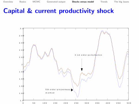
Capital & current productivity shock

0 5 0 1 0 0 1 5 0 2 0 0 2 5 0 3 0 0 3 5 0 4 0 0 4 5 0 5 0 01 . 9

1 . 9 2

1 . 9 4

1 . 9 6

1 . 9 8

2

2 . 0 2

2 . 0 4

2 . 0 6

2 . 0 8

2 . 1

2 ­n d   o rd e r   p e r t u rb a t i o n

5 t h ­o rd e r   p ro j e c t i o n s

m e t h o d

Overview Basics MCMC Generated output Shocks versus model Trends The big issues

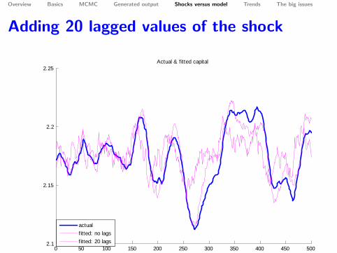
Adding 20 lagged values of the shock

0 50 100 150 200 250 300 350 400 450 5002.1

2.15

2.2

2.25Actual & fitted capital

actualfitted: no lagsfitted: 20 lags

Overview Basics MCMC Generated output Shocks versus model Trends The big issues

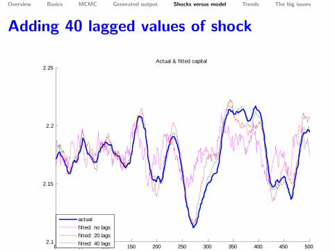
Adding 40 lagged values of shock

0 50 100 150 200 250 300 350 400 450 5002.1

2.15

2.2

2.25Actual & fitted capital

actualfitted: no lagsfitted: 20 lagsfitted: 40 lags

Overview Basics MCMC Generated output Shocks versus model Trends The big issues

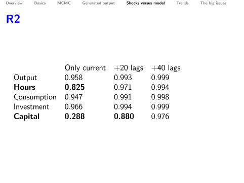
R2

Only current +20 lags +40 lagsOutput 0.958 0.993 0.999Hours 0.825 0.971 0.994Consumption 0.947 0.991 0.998Investment 0.966 0.994 0.999Capital 0.288 0.880 0.976

Overview Basics MCMC Generated output Shocks versus model Trends The big issues

Second example

• Christiano, Motto, Rostagno:• "Financial Factors in Economic Fluctuations"

• Quite complex model to model interaction between financialintermediation and real activity

Overview Basics MCMC Generated output Shocks versus model Trends The big issues

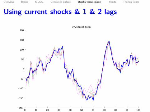
Using current shocks & 1 & 2 lags

0 10 20 30 40 50 60 70 80 90 100­200

­150

­100

­50

0

50

100

150

200CONSUMPTION

Overview Basics MCMC Generated output Shocks versus model Trends The big issues

Using current shocks & 1 & 2 lags

0 10 20 30 40 50 60 70 80 90 100­4000

­3000

­2000

­1000

0

1000

2000

3000

4000CREDIT

Overview Basics MCMC Generated output Shocks versus model Trends The big issues

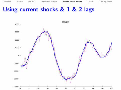
Using current shocks & 1 & 2 lags

0 10 20 30 40 50 60 70 80 90 100­0.02

­0.015

­0.01

­0.005

0

0.005

0.01

0.015DP

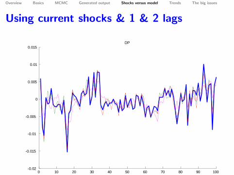
Overview Basics MCMC Generated output Shocks versus model Trends The big issues

Using current shocks & 1 & 2 lags

0 10 20 30 40 50 60 70 80 90 100­0.015

­0.01

­0.005

0

0.005

0.01

Dpip

Overview Basics MCMC Generated output Shocks versus model Trends The big issues

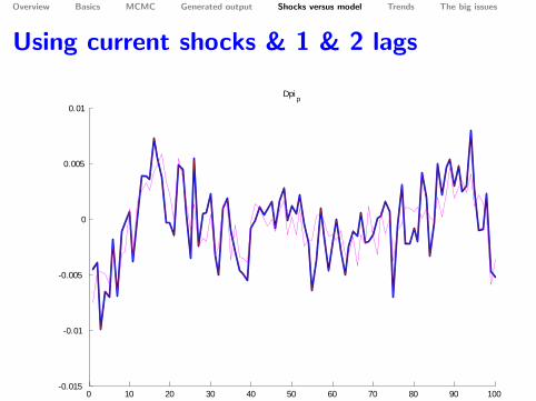
Using current shocks & 1 & 2 lags

0 10 20 30 40 50 60 70 80 90 100­0.6

­0.5

­0.4

­0.3

­0.2

­0.1

0

0.1

0.2

0.3

0.4OIL PRICE

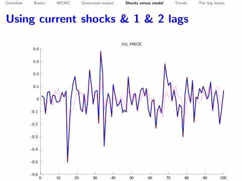
Overview Basics MCMC Generated output Shocks versus model Trends The big issues

Using current shocks & 1 & 2 lags

0 10 20 30 40 50 60 70 80 90 100­400

­300

­200

­100

0

100

200

300

400INVESTMENT

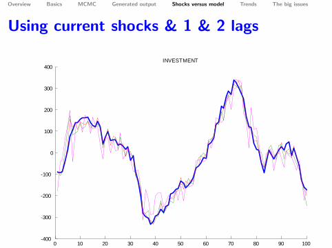
Overview Basics MCMC Generated output Shocks versus model Trends The big issues

Using current shocks & 1 & 2 lags

0 10 20 30 40 50 60 70 80 90 100­1000

­500

0

500

1000

1500M1

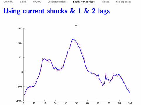
Overview Basics MCMC Generated output Shocks versus model Trends The big issues

Using current shocks & 1 & 2 lags

0 10 20 30 40 50 60 70 80 90 100­2500

­2000

­1500

­1000

­500

0

500

1000

1500

2000M3

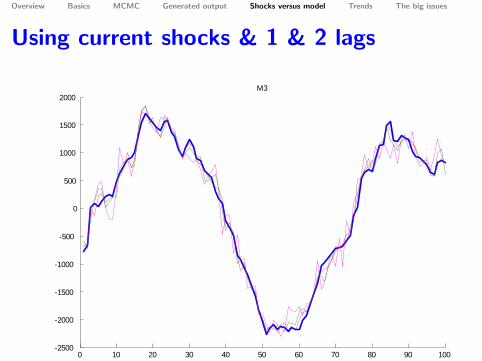
Overview Basics MCMC Generated output Shocks versus model Trends The big issues

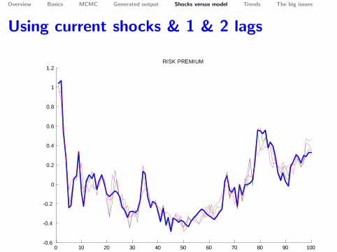
Using current shocks & 1 & 2 lags

0 10 20 30 40 50 60 70 80 90 100­0.6

­0.4

­0.2

0

0.2

0.4

0.6

0.8

1

1.2RISK PREMIUM

Overview Basics MCMC Generated output Shocks versus model Trends The big issues

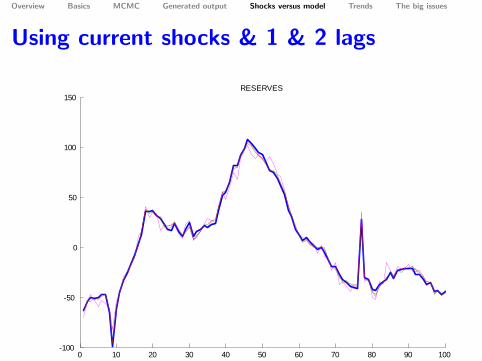
Using current shocks & 1 & 2 lags

0 10 20 30 40 50 60 70 80 90 100­100

­50

0

50

100

150RESERVES

Overview Basics MCMC Generated output Shocks versus model Trends The big issues

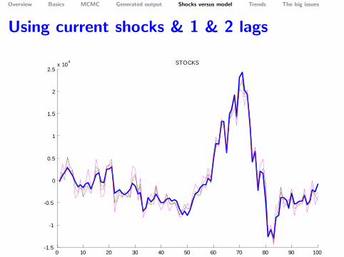
Using current shocks & 1 & 2 lags

0 10 20 30 40 50 60 70 80 90 100­1.5

­1

­0.5

0

0.5

1

1.5

2

2.5x 104 STOCKS

Overview Basics MCMC Generated output Shocks versus model Trends The big issues

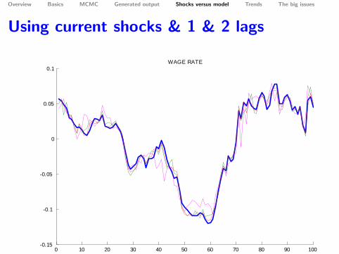
Using current shocks & 1 & 2 lags

0 10 20 30 40 50 60 70 80 90 100­0.15

­0.1

­0.05

0

0.05

0.1WAGE RATE

Overview Basics MCMC Generated output Shocks versus model Trends The big issues

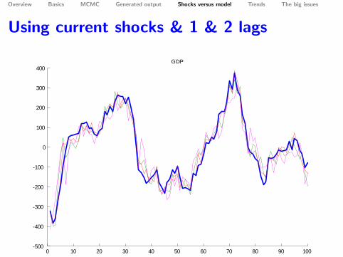
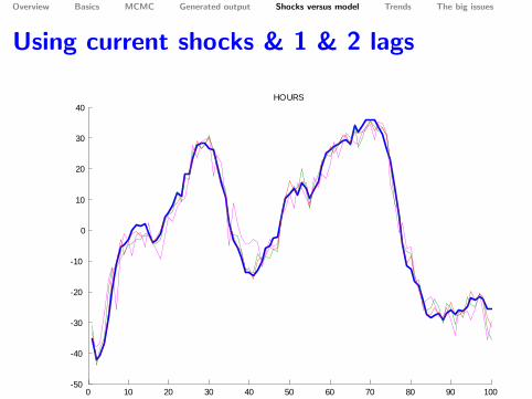
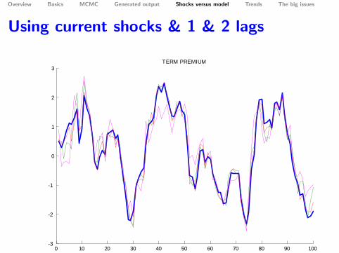
Using current shocks & 1 & 2 lags

0 10 20 30 40 50 60 70 80 90 100­500

­400

­300

­200

­100

0

100

200

300

400GDP

Overview Basics MCMC Generated output Shocks versus model Trends The big issues

Using current shocks & 1 & 2 lags

0 10 20 30 40 50 60 70 80 90 100­50

­40

­30

­20

­10

0

10

20

30

40HOURS

Overview Basics MCMC Generated output Shocks versus model Trends The big issues

Using current shocks & 1 & 2 lags

0 10 20 30 40 50 60 70 80 90 100­3

­2

­1

0

1

2

3TERM PREMIUM

Overview Basics MCMC Generated output Shocks versus model Trends The big issues

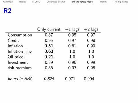
R2

Only current +1 lags +2 lagsConsumption 0.87 0.95 0.97Credit 0.95 0.97 0.98Inflation 0.51 0.81 0.90Inflation_inv 0.63 1.0 1.0Oil price 0.21 1.0 1.0Investment 0.89 0.96 0.99risk premium 0.86 0.93 0.98

hours in RBC 0.825 0.971 0.994

Overview Basics MCMC Generated output Shocks versus model Trends The big issues

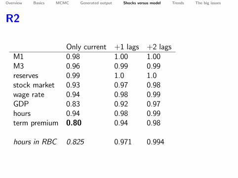
R2

Only current +1 lags +2 lagsM1 0.98 1.00 1.00M3 0.96 0.99 0.99reserves 0.99 1.0 1.0stock market 0.93 0.97 0.98wage rate 0.94 0.98 0.99GDP 0.83 0.92 0.97hours 0.94 0.98 0.99term premium 0.80 0.94 0.98

hours in RBC 0.825 0.971 0.994

Overview Basics MCMC Generated output Shocks versus model Trends The big issues

Shocks versus the model

• Is this bad?• Maybe not, but perceived wisdom– and the language in thepaper– suggests that propagation is very important

Overview Basics MCMC Generated output Shocks versus model Trends The big issues

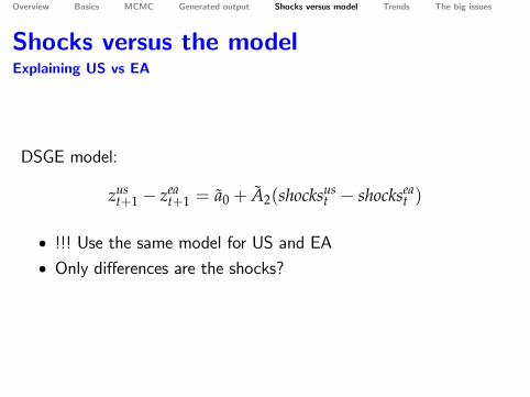
Shocks versus the modelExplaining US vs EA

DSGE model:

zust+1 − zea

t+1 = a0 + A2(shocksust − shocksea

t )

• !!! Use the same model for US and EA• Only differences are the shocks?

Overview Basics MCMC Generated output Shocks versus model Trends The big issues

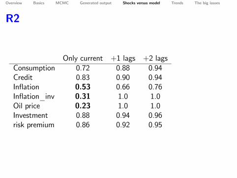
R2

Only current +1 lags +2 lagsConsumption 0.72 0.88 0.94Credit 0.83 0.90 0.94Inflation 0.53 0.66 0.76Inflation_inv 0.31 1.0 1.0Oil price 0.23 1.0 1.0Investment 0.88 0.94 0.96risk premium 0.86 0.92 0.95

Overview Basics MCMC Generated output Shocks versus model Trends The big issues

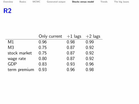
R2

Only current +1 lags +2 lagsM1 0.96 0.98 0.99M3 0.75 0.87 0.92stock market 0.75 0.87 0.92wage rate 0.80 0.87 0.92GDP 0.83 0.93 0.96term premium 0.93 0.96 0.98

Overview Basics MCMC Generated output Shocks versus model Trends The big issues

Very tricky issue

• Data have trends• Methodology works with stationary data

Overview Basics MCMC Generated output Shocks versus model Trends The big issues

Simple solution

• Put stochastic trend in model• Use first differences of model variables

Overview Basics MCMC Generated output Shocks versus model Trends The big issues

Disadvantages of the simple solution

• Info about level not used in estimation• e.g., consumption ≈ 2/3 output• =⇒ less parameters are identified

• ∆-filter emphasizes high frequency• measurement error shock could absorb this

• Not obvious how to put the right trend in model• Not obvious data are consistent with balanced growth

Overview Basics MCMC Generated output Shocks versus model Trends The big issues

Alternative I

Detrend data using

yt = a0 + a1t+ a2t2 + uy

Advantage

• Each observable can have its own trend

Overview Basics MCMC Generated output Shocks versus model Trends The big issues

Alternative II

Explicitly model trend as part of estimation problem

yobst = ytrendt + ymodelt

ytrendt = µ+ ytrendt−1 + ey,t

ymodelt is cyclical component determined by usual linearized equations

Advantage

• You can be very flexible in writing process for trend• Different variables can have different trends

Overview Basics MCMC Generated output Shocks versus model Trends The big issues

Alternative II

Same but written differently

y∗obst = ∆ytrendt + ∆ymodelt

∆ytrendt = µ+ ey,t

Overview Basics MCMC Generated output Shocks versus model Trends The big issues

Alternative III ??

Detrend data using HP or Band-Pass filter

yobs-filteredt = B(L)yobst

Problem

• B(L) is a two-sided filter =⇒ econometrically suspicious• yobs-filteredt has different properties than model data =⇒• apply same filter to model data

ymodel-filteredt = ymodelt

Overview Basics MCMC Generated output Shocks versus model Trends The big issues

Estimating misspecified models

• shocks versus observables• would wedges work?

Overview Basics MCMC Generated output Shocks versus model Trends The big issues

Alternatives to Bayesian estimation

• Maximum likelihood• Calibration• GMM• SMM & indirect inference

Overview Basics MCMC Generated output Shocks versus model Trends The big issues

References

• of course: www.dynare.org• Brooks, S.P. and A. Gelman, 1998, General methods for monitoringconvergence of iterative simulations, Journal of Computational andGraphical Statistics.

• Griffoli, T.M., Dynare user guide• Roberts, G.O., and A. Gelman, and W.R. Gilks, Weak convergenceand optimal scaling of random walk metropolis algorithms, TheAnnals of Applied Probability

• the "0.234" paper

• Roberts, G.O., and J.S. Rosenthal, 2004, General state spaceMarkov chains and MCMC algorithms, Probability Surveys.

• more advanced articles describing formal properties