Distributions of Critical Load in Arrays ofNanopillars

Zbigniew Domanski and Tomasz Derda

Abstract—Arrays of vertical pillars are encountered in a va-riety of nanotechnological applications, e.g. in sensing systems.If such an array of N pillars, with pillars characterized byrandom strength thresholds σth, is subjected to a sufficientlylarge axial load Fc, the pillars break in the form of cascadesof avalanches. Using a Fiber Bundle Model with a so-calledlocal load transfer rule from destroyed pillars to the intactones, we analyze distributions of Fc when thresholds σth areindependently drawn from the Weibull distribution, pk,λ(σth) =(k/λ)(σth/λ)k−1 exp[−(σth/λ)k], where λ = 1 and k are thescale and shape, respectively. Based on simulations we show thatdistribution of Fc/N = σc can be well fitted by the Weibull pdfpK,Λ(σc) = (K/Λ)(σc/Λ)K−1 exp[−(σc/Λ)K ], where K and Λare functions of k and N . Specifically, for N >> 1, the mean< Fc/N >∼ ln(k).

Index Terms—avalanche, array of pillars, critical load, frac-ture, probability distribution.

I. INTRODUCTION

A MODERN nanodevice may be composed of a largenumber of identical parts that function as a unit. A

possible sequence of failures among these components de-creases the device performance and may eventually lead toa catastrophic avalanche of failures.

Majority of studies dealing with avalanches of failuresemploy so-called load transfer models, as e.g., the FibreBundle Model (FBM) or Random Fuse Model [1], [2], [3].Especially the FBM, originally designed to describe loadedfibre bundles, can be applied to model damage processesin an array of vertical pillars regularly distributed on a flatsubstrate.

In this work, the array of pillars is represented by acollection of fibers and then analyzed within a static FibreBundle Model framework [4], [5], [6], [7], [8], [9]. Breakingof pillars from the support is a process involving avalanchesof fractures. This means that when a pillar breaks, its load istransferred to the other intact elements and thus the probabil-ity of subsequent fractures increases. Based on the results ofnumerical simulations, we claim that the observed weakeningof the axial load Fc is related to a load transfer phenomenonwhich is an inherent part of the fracture process in a bundleof pillars [8]. In our numerical experiment a set of N = L×Lpillars, located in the nodes of the supporting square lattice, issubjected to an axial load F . Defects significantly influencethe mechanical behaviour of materials under load. Due tothese defects, the pillar-strength-thresholds are modelled byquenched random variables. The two most popular strength-thresholds distributions are uniform distribution and Weibull

Manuscript received April 7, 2017.Z. Domanski is with the Institute of Mathematics, Czestochowa Uni-

versity of Technology, Dabrowskiego 69, PL-42201 Czestochowa, Poland.(corresponding author e-mail: zbigniew.domanski@im.pcz.pl).

T. Derda is with the Institute of Mathematics, Czestochowa Universityof Technology, Dabrowskiego 69, PL-42201 Czestochowa, Poland. (e-mail:tomasz.derda@im.pcz.pl).

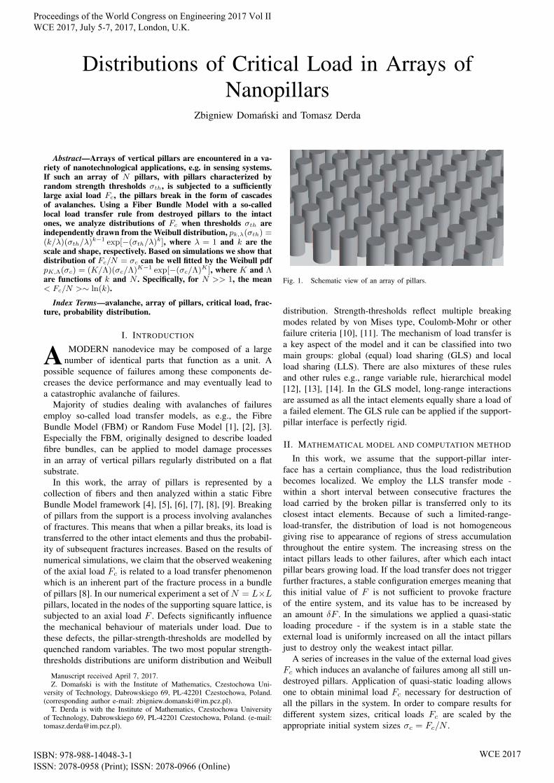
Fig. 1. Schematic view of an array of pillars.

distribution. Strength-thresholds reflect multiple breakingmodes related by von Mises type, Coulomb-Mohr or otherfailure criteria [10], [11]. The mechanism of load transfer isa key aspect of the model and it can be classified into twomain groups: global (equal) load sharing (GLS) and localload sharing (LLS). There are also mixtures of these rulesand other rules e.g., range variable rule, hierarchical model[12], [13], [14]. In the GLS model, long-range interactionsare assumed as all the intact elements equally share a load ofa failed element. The GLS rule can be applied if the support-pillar interface is perfectly rigid.

II. MATHEMATICAL MODEL AND COMPUTATION METHOD

In this work, we assume that the support-pillar inter-face has a certain compliance, thus the load redistributionbecomes localized. We employ the LLS transfer mode -within a short interval between consecutive fractures theload carried by the broken pillar is transferred only to itsclosest intact elements. Because of such a limited-range-load-transfer, the distribution of load is not homogeneousgiving rise to appearance of regions of stress accumulationthroughout the entire system. The increasing stress on theintact pillars leads to other failures, after which each intactpillar bears growing load. If the load transfer does not triggerfurther fractures, a stable configuration emerges meaning thatthis initial value of F is not sufficient to provoke fractureof the entire system, and its value has to be increased byan amount δF . In the simulations we applied a quasi-staticloading procedure - if the system is in a stable state theexternal load is uniformly increased on all the intact pillarsjust to destroy only the weakest intact pillar.

A series of increases in the value of the external load givesFc which induces an avalanche of failures among all still un-destroyed pillars. Application of quasi-static loading allowsone to obtain minimal load Fc necessary for destruction ofall the pillars in the system. In order to compare results fordifferent system sizes, critical loads Fc are scaled by theappropriate initial system sizes σc = Fc/N .

Proceedings of the World Congress on Engineering 2017 Vol II WCE 2017, July 5-7, 2017, London, U.K.

ISBN: 978-988-14048-3-1 ISSN: 2078-0958 (Print); ISSN: 2078-0966 (Online)

WCE 2017

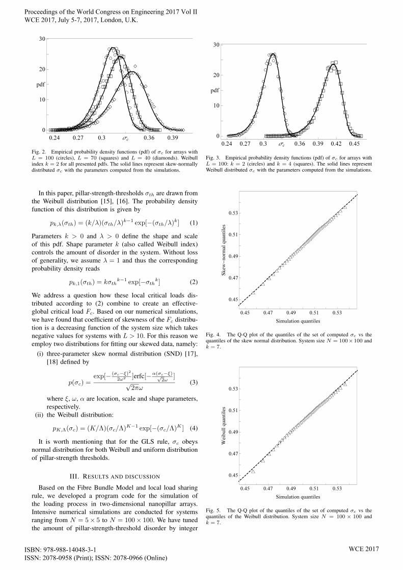
Fig. 2. Empirical probability density functions (pdf) of σc for arrays withL = 100 (circles), L = 70 (squares) and L = 40 (diamonds). Weibullindex k = 2 for all presented pdfs. The solid lines represent skew-normallydistributed σc with the parameters computed from the simulations.

In this paper, pillar-strength-thresholds σth are drawn fromthe Weibull distribution [15], [16]. The probability densityfunction of this distribution is given by

pk,λ(σth) = (k/λ)(σth/λ)k−1 exp[−(σth/λ)k] (1)

Parameters k > 0 and λ > 0 define the shape and scaleof this pdf. Shape parameter k (also called Weibull index)controls the amount of disorder in the system. Without lossof generality, we assume λ = 1 and thus the correspondingprobability density reads

pk,1(σth) = kσthk−1 exp[−σthk] (2)

We address a question how these local critical loads dis-tributed according to (2) combine to create an effective-global critical load Fc. Based on our numerical simulations,we have found that coefficient of skewness of the Fc distribu-tion is a decreasing function of the system size which takesnegative values for systems with L > 10. For this reason weemploy two distributions for fitting our skewed data, namely:

(i) three-parameter skew normal distribution (SND) [17],[18] defined by

p(σc) =exp[− (σc−ξ)2

2ω2 ]erfc[−α(σc−ξ)√2ω

]√

2πω(3)

where ξ, ω, α are location, scale and shape parameters,respectively.

(ii) the Weibull distribution:

pK,Λ(σc) = (K/Λ)(σc/Λ)K−1 exp[−(σc/Λ)K ] (4)

It is worth mentioning that for the GLS rule, σc obeysnormal distribution for both Weibull and uniform distributionof pillar-strength thresholds.

III. RESULTS AND DISCUSSION

Based on the Fibre Bundle Model and local load sharingrule, we developed a program code for the simulation ofthe loading process in two-dimensional nanopillar arrays.Intensive numerical simulations are conducted for systemsranging from N = 5× 5 to N = 100× 100. We have tunedthe amount of pillar-strength-threshold disorder by integer

Fig. 3. Empirical probability density functions (pdf) of σc for arrays withL = 100: k = 2 (circles) and k = 4 (squares). The solid lines representWeibull distributed σc with the parameters computed from the simulations.

Fig. 4. The Q-Q plot of the quantiles of the set of computed σc vs thequantiles of the skew normal distribution. System size N = 100×100 andk = 7.

Fig. 5. The Q-Q plot of the quantiles of the set of computed σc vs thequantiles of the Weibull distribution. System size N = 100 × 100 andk = 7.

Proceedings of the World Congress on Engineering 2017 Vol II WCE 2017, July 5-7, 2017, London, U.K.

ISBN: 978-988-14048-3-1 ISSN: 2078-0958 (Print); ISSN: 2078-0966 (Online)

WCE 2017

values of k ranging from 2 to 9. In order to get reliablestatistics, each simulation was repeated 104 times.

Figures 2 and 3 show empirical probability density func-tions of σc for chosen systems. In these plots we have alsoadded fitting lines of skew normal (Fig. 2) and Weibull (Fig.3) probability density functions with parameters computedfrom the samples. It can be seen that both of these theo-retical distributions are in good agreement with empiricaldistributions of σc. We also present a quantile-quantile plot(Q-Q plot) of the quantiles of the collected data set againstthe corresponding quantiles given by the SND and Weibullprobability distributions. From Figures 4 and 5, it is seen thatthe result of fitting by skew normal distribution is slightlybetter than the Weibull fitting. Based on simulations, wehave observed that fitting by skew normal distribution givesbetter results than Weibull fitting for all analysed systems,especially for the smaller ones. However, it should be notedthat skew normal distribution has one parameter more thanWeibull distribution. Fitting by Weibull distribution allows usto analyse the influence of system properties on the micro-scopic level (Weibull distributed pillar-strength thresholds)on the macroscopic response (distribution of crical loads) inthe framework of one type of distribution. Hence, we focusour attention on the fitting of σc distribution by Weibulldistribution.

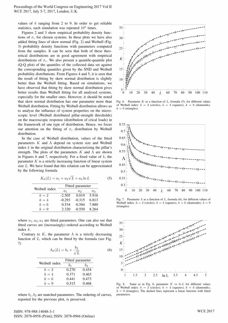
In the case of Weibull distribution, values of the fittedparameters K and Λ depend on system size and Weibullindex k in the original distribution characterizing the pillar’sstrength. The plots of the parameters K and Λ are shownin Figures 6 and 7, respectively. For a fixed value of k, theparameter K is a strictly increasing function of linear systemsize L. We have found that this relation can be approximatedby the following formula

Kk(L) = a1 + a2

√L+ a3 lnL (5)

Fitted parameterWeibull index a1 a2 a3

k = 2 -2.505 0.019 5.916k = 4 -0.293 -0.315 6.813k = 6 0.534 -0.584 7.880k = 9 2.320 -0.550 8.264

where a1, a2, a3 are fitted parameters. One can also see thatfitted curves are (increasingly) ordered according to Weibullindex k.

Contrary to K, the parameter Λ is a strictly decreasingfunction of L, which can be fitted by the formula (see Fig.7)

Λk(L) = b1 +b2√L

(6)

Fitted parameterWeibull index b1 b2

k = 2 0.270 0.454k = 4 0.371 0.463k = 6 0.441 0.473k = 9 0.515 0.468

where b1, b2 are matched parameters. The ordering of curves,reported for the previous plot, is preserved.

Fig. 6. Parameter K as a function of L, formula (5), for different valuesof Weibull index: k = 2 (circles), k = 4 (squares), k = 6 (diamonds),k = 9 (triangles).

Fig. 7. Parameter Λ as a function of L, formula (6), for different values ofWeibull index: k = 2 (circles), k = 4 (squares), k = 6 (diamonds), k = 9(triangles).

Fig. 8. Same as in Fig. 6, parameter K vs lnL for different valuesof Weibull index: k = 2 (circles), k = 4 (squares), k = 6 (diamonds),k = 9 (triangles). The dashed lines represent a linear function with fittedparameters.

Proceedings of the World Congress on Engineering 2017 Vol II WCE 2017, July 5-7, 2017, London, U.K.

ISBN: 978-988-14048-3-1 ISSN: 2078-0958 (Print); ISSN: 2078-0966 (Online)

WCE 2017

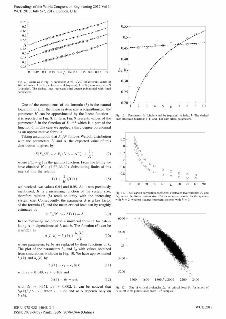
Fig. 9. Same as in Fig. 7, parameter Λ vs 1/√L for different values of

Weibull index: k = 2 (circles), k = 4 (squares), k = 6 (diamonds), k = 9(triangles). The dashed lines represent third degree polynomial with fittedparameters.

One of the components of the formula (5) is the naturallogarithm of L. If the linear system size is logarithmized, theparameter K can be approximated by the linear function -it is reported in Fig. 8. In turn, Fig. 9 presents values of theparameter Λ in the function of L−1/2 which is a part of thefunction 6. In this case we applied a third degree polynomialas an approximative formula.

Taking assumption that Fc/N follows Weibull distributionwith the parameters K and Λ, the expected value of thisdistribution is given by

E[Fc/N ] =< Fc/N >= ΛΓ(1 +1

K) (7)

where Γ(1 + 1K ) is the gamma function. From the fitting we

have obtained K ∈ (7.27, 33.69). Substituting limits of thisinterval into the relation

Γ(1 +1

K)/Γ(1) (8)

we received two values 0.94 and 0.98. As it was previouslymentioned, K is a increasing function of the system size,therefore relation (8) tends to unity with the increasingsystem size. Consequently, the parameter Λ is a key factorof the formula (7) and the mean critical load can by roughlyestimated by

< Fc/N >∼ ΛΓ(1) = Λ (9)

In the following we propose a universal formula for calcu-lating Λ in dependence of L and k. The function (6) can berewritten as

Λ(L, k) = b1(k) +b2(k)√L

(10)

where parameters b1, b2 are replaced by their functions of k.The plot of the parameters b1 and b2 with values obtainedfrom simulations is shown in Fig. 10. We have approximatedb1(k) and b2(k) by

b1(k) = c1 + c2 ln k (11)

with c1 ≈ 0.148, c2 ≈ 0.165 and

b2(k) = d1 + d2k (12)

with d1 ≈ 0.451, d2 ≈ 0.002. It can be noticed thatb2(k)/

√L → 0 when L → ∞ and so Λ depends only on

b1(k).

Fig. 10. Parameters b1 (circles) and b2 (squares) vs index k. The dashedlines illustrate functions (11) and (12) with fitted parameters.

Fig. 11. The Pearson correlation coefficient r between two variables Fc and∆c versus the linear system size. Circles represent results for the systemswith k = 2, whereas squares represent systems with k = 9.

Fig. 12. Size of critical avalanche ∆c vs critical load Fc for arrays ofN = 80× 80 pillars taken from 104 samples.

Proceedings of the World Congress on Engineering 2017 Vol II WCE 2017, July 5-7, 2017, London, U.K.

ISBN: 978-988-14048-3-1 ISSN: 2078-0958 (Print); ISSN: 2078-0966 (Online)

WCE 2017

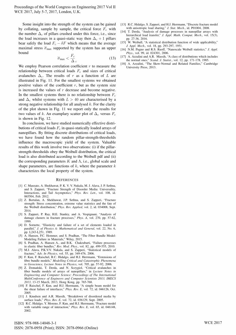
Some insight into the strength of the system can be gainedby collating, sample by sample, the critical force Fc withthe number ∆c of pillars crushed under this force, i.e., sincethe load increases in a quasi-static way then ∆c + 1 pillarsbear safely the load Fc − δF which means that the averagemaximal stress σmax supported by the system has an upperbound

σmax <Fc∆ c

(13)

We employ Pearson correlation coefficient r to measure therelationship between critical loads Fc and sizes of criticalavalanches ∆c. The results of r as a function of L areillustrated in Fig. 11. For the smallest systems we obtainedpositive values of the coefficient r, but as the system sizeis increased the values of r decrease and become negative.In the smallest systems there is no relationship between Fcand ∆c whilst systems with L > 40 are characterised by astrong negative relationship for all analysed k. For the clarityof the plot shown in Fig. 11 we report only the results fortwo values of k. An examplary scatter plot of ∆c versus Fcis shown in Fig. 12.

In conclusion, we have studied numerically effective distri-butions of critical loads Fc in quasi-statically loaded arrays ofnanopillars. By fitting discrete distributions of critical loads,we have found how the random pillar-strength-thresholdsinfluence the macroscopic yield of the system. Valuableresults of this work involve two observations: (i) if the pillar-strength-thresholds obey the Weibull distribution, the criticalload is also distributed according to the Weibull pdf and (ii)the corresponding parameters K and Λ, i.e., global scale andshape parameters, are functions of k, where the parameter kcharacterizes the local property of the system.

REFERENCES

[1] C. Manzato, A. Shekhawat, P. K. V. V. Nukala, M. J. Alava, J. P. Sethna,and S. Zapperi, “Fracture Strength of Disorder Media: Universality,Interactions, and Tail Asymptotics,” Phys. Rev. Lett., vol. 108, id.065504, Feb. 2012.

[2] Z. Bertalan, A. Shekhawat, J.P. Sethna, and S. Zapperi, “Fracturestrength: Stress concentration, extreme value statistics and the fate ofthe Weibull distribution,” Phys. Rev. Applied, vol. 2, id. 034008, Sept.2014.

[3] S. Zapperi, P. Ray, H.E. Stanley, and A. Vespignani, “Analysis ofdamage clusters in fracture processes,” Phys. A, vol. 270, pp. 57-62,1999.

[4] D. Sornette, “Elasticity and failure of a set of elements loaded inparallel,” J. of Physics A: Mathematical and General, vol. 22, No. 6,pp. L243-L251, 1989.

[5] A. Hansen, P.C. Hemmer, and S. Pradhan, “The Fiber Bundle Model:Modeling Failure in Materials,” Wiley, 2015.

[6] S. Pradhan, A. Hansen A., and B.K. Chakrabarti, “Failure processesin elastic fiber bundles,” Rev. Mod. Phys., vol. 82, pp. 499-555, 2010.

[7] M.J. Alava, P.K.V.V. Nukala, and S. Zapperi, “Statistical models offracture,” Adv. In Physics, vol. 55, pp. 349-476, 2006.

[8] F. Kun, F. Raischel, R.C. Hidalgo, and H.J. Herrmann, “Extensions offibre bundle models,” Modelling Critical and Catastrophic Phenomenain Geoscience, Lecture Notes in Physics, vol. 705, pp. 57-92, 2006.

[9] Z. Domanski, T. Derda, and N. Sczygiol, “Critical avalanches infiber bundle models of arrays of nanopillars,” in Lecture Notes inEngineering and Computer Science: Proceedings of The InternationalMultiConference of Engineers and Computer Scientists 2013, IMECS2013, 13-15 March, 2013, Hong Kong, pp. 765-768.

[10] F. Raischel, F. Kun, and H.J. Herrmann, “A simple beam model forthe shear failure of interfaces,” Phys. Rev. E, vol. 72, id. 046126, Oct.2005.

[11] J. Knudsen and A.R. Massih, “Breakdown of disordered media bysurface loads,” Phys. Rev. E, vol. 72, id. 036129, Sept. 2005.

[12] R.C. Hidalgo, Y. Moreno, F. Kun, and H.J. Herrmann, “Fracture modelwith variable range of interaction,” Phys. Rev. E, vol. 65, id. 046148,2002.

[13] R.C. Hidalgo, S. Zapperi, and H.J. Herrmann, “Discrete fracture modelwith anisotropic load sharing,” J. Stat. Mech., id. P01004, 2008.

[14] T. Derda, “Analysis of damage processes in nanopillar arrays withhierarchical load transfer,” J. Appl. Math. Comput. Mech., vol. 15(3),pp. 27-36, 2016.

[15] W. Weibull, “A statistical distribution function of wide applicability,”J. Appl. Mech., vol. 18, pp. 293-297, 1951.

[16] N.M. Pugno and R.S. Ruoff, “Nanoscale Weibull statistics,” J. Appl.Phys., vol. 99, id. 024301, 2006.

[17] A. Azzalini and A.R. Massih, “A class of distributions which includesthe normal ones,” Scand. J. Statist., vol. 12, pp. 171-178, 1985.

[18] A. Azzalini, “The Skew-Normal and Related Families,” CambridgeUniversity Press, 2013.

Proceedings of the World Congress on Engineering 2017 Vol II WCE 2017, July 5-7, 2017, London, U.K.

ISBN: 978-988-14048-3-1 ISSN: 2078-0958 (Print); ISSN: 2078-0966 (Online)

WCE 2017