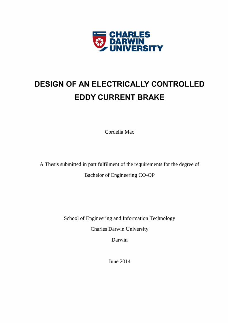
DESIGN OF AN ELECTRICALLY CONTROLLED

EDDY CURRENT BRAKE

Cordelia Mac

A Thesis submitted in part fulfilment of the requirements for the degree of

Bachelor of Engineering CO-OP

School of Engineering and Information Technology

Charles Darwin University

Darwin

June 2014

Design of an Electrically Controlled Eddy Current Brake i

Abstract

Keywords: Eddy Current Brake Design, Wouterse, Torque, Speed, Current,

Eddy current brakes (ECB) utilise electromagnets to generate smooth braking torque in contrast

with traditional friction braking. A disadvantage is the low braking forces experienced at low

speeds and as a consequence, the moving object never ceases its motion.

The aim of this research is to develop and construct an electrically controlled ECB for research

on an application specific motor at Charles Darwin University (CDU).

A literature review was conducted into previous works on ECBs and three theoretical models

were identified. Between the models Schieber, Smythe and Wouterse, the Wouterse method

appeared most appropriate as it is both simple and applicable for this application.

The determination of the magnetisation curve of the core material provides the characteristics

required to design the ECB. The load line was determined for specific currents to provide a

theoretical flux density in the air gap. These values were also confirmed experimentally. The

design indicated that in order to achieve the required specifications and constraints, a large

number of turns and core would be required. The final constructed design was tested using the

permanent magnet synchronous motor (PMSM) at CDU to confirm the simulated torque, speed

and current values.

In order to confirm the flux travelling through the air gap, a Gaussmeter was used to

experimentally measure the flux. The results for the torque versus speed was collected using

Labview. This provided torque and speed readings through a torque sensor and incremental

encoder. As the aluminium disc did not completely occupy the cross sectional area of the core’s

air gap, the results confirm that in order to achieve the simulated results, the current required

will need to be increased.

Design of an Electrically Controlled Eddy Current Brake ii

Acknowledgments

I would like to express my appreciation to my supervisor Damien Hill for his patience,

guidance, encouragement and useful critique throughout this thesis. I would also like to thank

Chris Lugg for being my co-supervisor and for being available to discuss mechanical related

aspects in this thesis. Special thanks to Ben Saunders for critiquing my ideas. Finally, I would

like to thank my parents, siblings and partner for their encouragement throughout my studies.

Design of an Electrically Controlled Eddy Current Brake iii

Contents

1 Introduction ........................................................................................................... 1

1.1 Aim of the Research....................................................................................... 1

1.2 Constraints ..................................................................................................... 2

1.3 Research Approach ........................................................................................ 2

1.4 Overview of Chapters .................................................................................... 2

2 Literature Review .................................................................................................. 3

2.1 Electromagnetic Theory ................................................................................. 3

2.1.1 Maxwell’s Second Equation ................................................................... 3

2.1.2 Magnetic Circuits ................................................................................... 4

2.2 Back Electromotive Forces (Back EMF) ....................................................... 7

2.3 Eddy Current Brakes (ECBs) ......................................................................... 7

2.3.1 Models .................................................................................................. 10

2.4 Finite Element Analysis (FEA) .................................................................... 15

3 Determination of Magnetisation Curve ............................................................... 17

4 Final Design ........................................................................................................ 24

4.1 Calculations: ................................................................................................ 25

4.1.1 Corresponding Flux Density used in Torque Calculations ................... 25

4.2 Critical Speed ............................................................................................... 30

4.3 Design trade-offs .......................................................................................... 31

4.4 Construction ................................................................................................. 32

4.5 Experimental Set-up..................................................................................... 34

5 Results ................................................................................................................. 36

5.1 Validity of assumptions ............................................................................... 36

5.2 Eddy Current Brake Testing Results............................................................ 36

5.2.1 Torque Offset ........................................................................................ 36

5.2.2 Testing .................................................................................................. 37

5.3 Discussion .................................................................................................... 43

5.3.1 Experimental set-up .............................................................................. 43

5.4 Improvements .............................................................................................. 45

5.5 Summary of results ...................................................................................... 46

6 Conclusion ........................................................................................................... 47

7 Future Works ....................................................................................................... 48

Design of an Electrically Controlled Eddy Current Brake iv

8 References ........................................................................................................... 50

Appendices ................................................................................................................. 52

Appendix A: Matlab Files ....................................................................................... 52

Appendix B: Calculations for 1000 and 2000 turns................................................ 59

Appendix C: Proposed Design ................................................................................ 61

Design of an Electrically Controlled Eddy Current Brake v

List of Symbols

φ = Flux (Wb)

�⃗� = Magnetic Flux Density (Tesla (T))

∆𝑠 = Surface

∇ = Used to represent a 3 dimensional vector �⃗� (x,y,z)

B = Magnetic flux intensity produced by Eddy Currents (Wb)

B’ = Magnetic flux of an external field (Wb)

γ = Electric conductivity (in the x-y plane for Equation 5) (Siemens/metre S/m)

𝐸𝑏 = Back EMF (V)

𝐾𝑣 = Back EMF constant

ω = Angular velocity (rad/s)

ρ = resistivity of the material (ohm-metre - Ωm)

𝜏𝑑 = Braking torque (N.m)

𝑃𝑑 = Power dissipated (W)

�̇� = Velocity of disc (m/s)

𝑑 𝑜𝑟 𝑏 (Equation 17) 𝑜𝑟 𝑡 = disc thickness (m)

D = Diameter of the magnet core (m)

R or m= Distance pole is from centre of disc (m)

σ = Conductivity of material (disc) (Siemens/metre S/m)

𝜇0= Permeability of free air (4𝜋 ∗ 10−7 𝐻𝑚−1)

E = Electric Field intensity (Newtons/Coulomb – N/C)

𝑣 = Velocity (m/s)

Design of an Electrically Controlled Eddy Current Brake vi

T= Torque (Equation 15)

R = Reluctance in Equation 11(At/wb)

𝜑0 = Flux penetrating the sheet at rest (Maxwells) (10−8 𝑤𝑒𝑏𝑒𝑟𝑠)

𝛿 = Sheet thickness (m)

R = Radius of electromagnet (m) in Equation 15

a or r = Disc radius (m)

a and B ( Equation 17) = Cross sectional width and length of core respectively (m)

l= Mean length of core (m)

i= Excitation current of coil (A)

N = Number of turns

Design of an Electrically Controlled Eddy Current Brake vii

List of Tables

Table 1 Copper excess against proportionality factor c for low speed dragging force [21] ..... 13

Table 2 Comparison of Flux Density Values ........................................................................... 28

Table 3 Relationship between Current and Number of Turns .................................................. 31

Table 4 Configuration Table for 2 coils ................................................................................... 32

Table 5 Current for 1000 turns ................................................................................................. 59

Table 6 Current for 2000 turns ................................................................................................. 60

Design of an Electrically Controlled Eddy Current Brake viii

List of Figures

Figure 1 Right-hand rule [4] ....................................................................................................... 4

Figure 2 Flux density distribution between two permanent magnets [6] ................................... 5

Figure 3 Magnetization Curve [4] .............................................................................................. 6

Figure 4 Determination of B due to air gap [8] .......................................................................... 7

Figure 5 Mathcad Model torque/speed curve, final design, 10 A coil current [19] ................... 9

Figure 6 Lines of Flow of Eddy Currents induced in rotating disc by two circular pole magnets

[2].............................................................................................................................................. 11

Figure 7 Torque versus speed for large disc rotating between four rectangular pole pairs of an

electromagnet measured by Lentz[2] ....................................................................................... 12

Figure 8 Diagram of Eddy Current Brake Variables [10] ........................................................ 14

Figure 9 Relationship between voltage, current and number of turns ...................................... 18

Figure 10 Magnetisation Curve Set up [29] ............................................................................. 19

Figure 11 Experimental set up .................................................................................................. 19

Figure 12 Main coil current vs. sensing voltage ....................................................................... 20

Figure 13 Hysteresis Curve ...................................................................................................... 21

Figure 14 BH Curve with all points.......................................................................................... 22

Figure 15 BH Curve ................................................................................................................. 23

Figure 16 Eddy Current Brake Experimental Set-Up [21] ....................................................... 24

Figure 17 determining the corresponding flux for a given current ........................................... 27

Figure 18 Torque vs. Speed (via Experimental BH Curve values) restricted at 3Nm ............. 29

Figure 19 2000 turn electromagnet prior to fibreglass encasement .......................................... 33

Design of an Electrically Controlled Eddy Current Brake ix

Figure 20 Fibreglass encasement .............................................................................................. 34

Figure 21 Experimental Set-up ................................................................................................. 35

Figure 22 Amount of aluminium disc present in the electromagnet ........................................ 35

Figure 23 Offsets observed in experimental data ..................................................................... 37

Figure 24 0.1A for experimental data, theoretical with and without factors ............................ 38

Figure 25 0.2A for experimental data, theoretical with and without factors ............................ 38

Figure 26 0.3A for experimental data, theoretical with and without factors ............................ 39

Figure 27 0.4A for experimental data, theoretical with and without factors ............................ 39

Figure 28 0.5A for experimental data, theoretical with and without factors ............................ 40

Figure 29 1.0A for experimental data, theoretical with and without factors ............................ 40

Figure 30 2.0A for experimental data, theoretical with and without factors ............................ 41

Figure 31 3.0A for experimental data, theoretical with and without factors ............................ 41

Figure 32 4.0A for experimental data, theoretical with and without factors ............................ 42

Figure 33 5.0A for experimental data, theoretical with and without factors ............................ 42

Design of an Electrically Controlled Eddy Current Brake 1

1 Introduction

Charles Darwin University (CDU) has conducted experimental research on minimising the

torque ripple experienced by permanent magnet synchronous motors (PMSM). However, the

load is manually adjusted and therefore, for this test system, the load is unknown. An

electromagnetic braking system, such as an eddy current brake (ECB), can provide a known

time-varying load with a certain bandwidth, a frictionless braking system and known

parameters for the PMSM research.

An electromagnetic braking system such as an ECB consists of a core with a small air gap, and

a rotating disc with conductive properties. This coil encases a core material which has magnetic

properties. The number of turns in the coil is dependent on the desired magnetic field strength

and braking force. Eddy currents produce an opposing magnetic field to slow down an object

such as a conductive rotating disc. These forces are created by inducing a current through the

coil when a disc, with conductive properties rotate within the air gap. The magnitude of these

forces is dependent on the conductivity of the conductor and the rate the magnetic field changes.

This thesis will detail the development and construction of an electrically controlled ECB for a

known load provided by the axial flux PMSM.

The structure of this thesis will consist of conducting the following:

Literature review on previous works with ECB,

Design to meet the specified requirements prior to the construction of the ECB itself,

Discussion of results which will confirm the accuracy of the theoretical design

parameters,

Recommendations for suggested future works.

1.1 Aim of the Research

The aim of this research is to develop and construct an electrically controlled ECB for a specific

application motor under research at CDU.

Design of an Electrically Controlled Eddy Current Brake 2

1.2 Constraints

The constraints of this thesis include the following:

Torque of a minimum value of 0.3 Nm

Voltage restriction of 60V DC

Frequency must be able to be analysed from 1Hz to 10Hz

1.3 Research Approach

Completion of the research goal involved the following tasks:

1. A literature review of:

Published ECB Models

Magnetic Circuits

2. Experimentation of:

Magnetisation Curve (Hysteresis and B-H Curve)

3. Design of the ECB

4. Construction of ECB and discussion of results

5. Conclusions

6. Future works

1.4 Overview of Chapters

Chapter 2 is separated into the electromagnetic theory, back electromotive forces, ECBs and

finite element analysis. Chapter 3 details the determination of the magnetisation curve for the

core material which will be used in the construction of the ECB. The importance of this chapter

will be further discussed in Chapter 4.1. Chapter 4 details the design stages which will be

undertaken to achieve a working model of the ECB. Chapter 5 details the findings and

discussion for the experimentation of the ECB. The findings from this chapter will provide

recommendations for further research in chapter 7.

Design of an Electrically Controlled Eddy Current Brake 3

2 Literature Review

2.1 Electromagnetic Theory

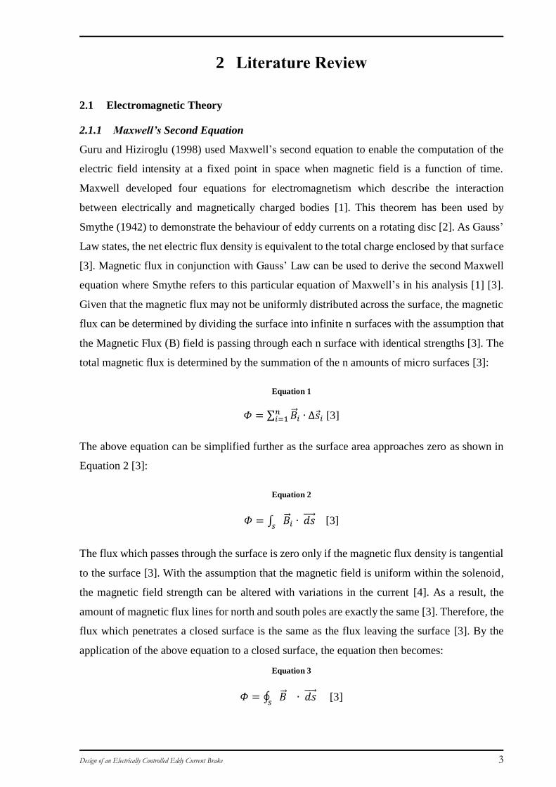
2.1.1 Maxwell’s Second Equation

Guru and Hiziroglu (1998) used Maxwell’s second equation to enable the computation of the

electric field intensity at a fixed point in space when magnetic field is a function of time.

Maxwell developed four equations for electromagnetism which describe the interaction

between electrically and magnetically charged bodies [1]. This theorem has been used by

Smythe (1942) to demonstrate the behaviour of eddy currents on a rotating disc [2]. As Gauss’

Law states, the net electric flux density is equivalent to the total charge enclosed by that surface

[3]. Magnetic flux in conjunction with Gauss’ Law can be used to derive the second Maxwell

equation where Smythe refers to this particular equation of Maxwell’s in his analysis [1] [3].

Given that the magnetic flux may not be uniformly distributed across the surface, the magnetic

flux can be determined by dividing the surface into infinite n surfaces with the assumption that

the Magnetic Flux (B) field is passing through each n surface with identical strengths [3]. The

total magnetic flux is determined by the summation of the n amounts of micro surfaces [3]:

Equation 1

𝛷 = ∑ �⃗� 𝑖 ∙ ∆𝑠 𝑖𝑛𝑖=1 [3]

The above equation can be simplified further as the surface area approaches zero as shown in

Equation 2 [3]:

Equation 2

𝛷 = ∫ �⃗� 𝑖 ∙ 𝑑𝑠⃗⃗⃗⃗ 𝑠

[3]

The flux which passes through the surface is zero only if the magnetic flux density is tangential

to the surface [3]. With the assumption that the magnetic field is uniform within the solenoid,

the magnetic field strength can be altered with variations in the current [4]. As a result, the

amount of magnetic flux lines for north and south poles are exactly the same [3]. Therefore, the

flux which penetrates a closed surface is the same as the flux leaving the surface [3]. By the

application of the above equation to a closed surface, the equation then becomes:

Equation 3

𝛷 = ∮ �⃗� ∙ 𝑑𝑠⃗⃗⃗⃗ 𝑠

[3]

Design of an Electrically Controlled Eddy Current Brake 4

Using the divergence theorem, the closed surface integral can be converted into a volume

integral. The volume under consideration is not always equal to zero. [3] The final equation can

be written as:

Equation 4

∇ ∙ �⃗� = 0 [3]

The above equation is known as Gauss’ Law of magnetic fields and demonstrates that the

magnetic flux density is solenoidal due to the divergence of B which equals zero at all points

of in the field [3]. Smythe determines the boundaries by combining Maxwell’s first equation

with ohm’s law and writing out the z components to give:

Equation 5

±𝜕𝐵𝑧

′+𝐵𝑧

𝜕𝑡=

1

2𝜋𝑏𝛾 𝜕𝐵𝑧

𝜕𝑧 [2]

Equation 6

∇ 𝑋 𝐵 = 0 [2]

By combining Equation 4 with Equation 5 and Equation 6 , B will be determined [2].

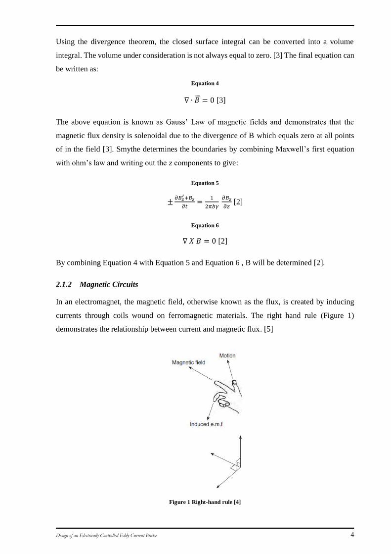
2.1.2 Magnetic Circuits

In an electromagnet, the magnetic field, otherwise known as the flux, is created by inducing

currents through coils wound on ferromagnetic materials. The right hand rule (Figure 1)

demonstrates the relationship between current and magnetic flux. [5]

Figure 1 Right-hand rule [4]

Design of an Electrically Controlled Eddy Current Brake 5

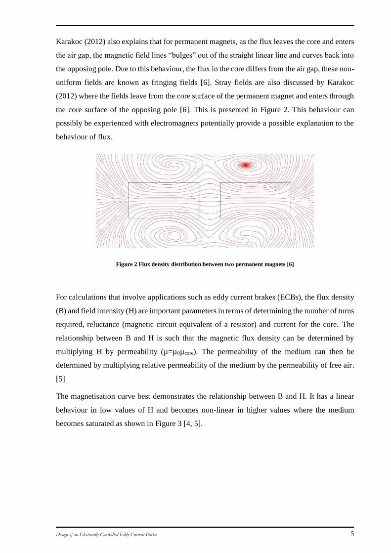
Karakoc (2012) also explains that for permanent magnets, as the flux leaves the core and enters

the air gap, the magnetic field lines “bulges” out of the straight linear line and curves back into

the opposing pole. Due to this behaviour, the flux in the core differs from the air gap, these non-

uniform fields are known as fringing fields [6]. Stray fields are also discussed by Karakoc

(2012) where the fields leave from the core surface of the permanent magnet and enters through

the core surface of the opposing pole [6]. This is presented in Figure 2. This behaviour can

possibly be experienced with electromagnets potentially provide a possible explanation to the

behaviour of flux.

Figure 2 Flux density distribution between two permanent magnets [6]

For calculations that involve applications such as eddy current brakes (ECBs), the flux density

(B) and field intensity (H) are important parameters in terms of determining the number of turns

required, reluctance (magnetic circuit equivalent of a resistor) and current for the core. The

relationship between B and H is such that the magnetic flux density can be determined by

multiplying H by permeability (µ=µ0µcore). The permeability of the medium can then be

determined by multiplying relative permeability of the medium by the permeability of free air.

[5]

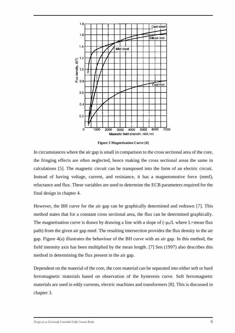
The magnetisation curve best demonstrates the relationship between B and H. It has a linear

behaviour in low values of H and becomes non-linear in higher values where the medium

becomes saturated as shown in Figure 3 [4, 5].

Design of an Electrically Controlled Eddy Current Brake 6

Figure 3 Magnetization Curve [4]

In circumstances where the air gap is small in comparison to the cross sectional area of the core,

the fringing effects are often neglected, hence making the cross sectional areas the same in

calculations [5]. The magnetic circuit can be transposed into the form of an electric circuit.

Instead of having voltage, current, and resistance, it has a magnetomotive force (mmf),

reluctance and flux. These variables are used to determine the ECB parameters required for the

final design in chapter 4.

However, the BH curve for the air gap can be graphically determined and redrawn [7]. This

method states that for a constant cross sectional area, the flux can be determined graphically.

The magnetisation curve is drawn by drawing a line with a slope of (-µ0/L where L=mean flux

path) from the given air gap mmf. The resulting intersection provides the flux density in the air

gap. Figure 4(a) illustrates the behaviour of the BH curve with an air gap. In this method, the

field intensity axis has been multiplied by the mean length. [7] Sen (1997) also describes this

method in determining the flux present in the air gap.

Dependent on the material of the core, the core material can be separated into either soft or hard

ferromagnetic materials based on observation of the hysteresis curve. Soft ferromagnetic

materials are used in eddy currents, electric machines and transformers [8]. This is discussed in

chapter 3.

Design of an Electrically Controlled Eddy Current Brake 7

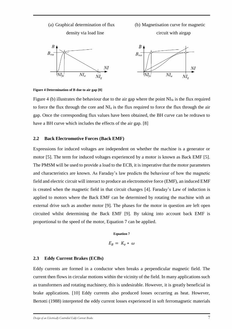
(a) Graphical determination of flux

density via load line

(b) Magnetisation curve for magnetic

circuit with airgap

Figure 4 Determination of B due to air gap [8]

Figure 4 (b) illustrates the behaviour due to the air gap where the point NIfe is the flux required

to force the flux through the core and NIa is the flux required to force the flux through the air

gap. Once the corresponding flux values have been obtained, the BH curve can be redrawn to

have a BH curve which includes the effects of the air gap. [8]

2.2 Back Electromotive Forces (Back EMF)

Expressions for induced voltages are independent on whether the machine is a generator or

motor [5]. The term for induced voltages experienced by a motor is known as Back EMF [5].

The PMSM will be used to provide a load to the ECB, it is imperative that the motor parameters

and characteristics are known. As Faraday’s law predicts the behaviour of how the magnetic

field and electric circuit will interact to produce an electromotive force (EMF), an induced EMF

is created when the magnetic field in that circuit changes [4]. Faraday’s Law of induction is

applied to motors where the Back EMF can be determined by rotating the machine with an

external drive such as another motor [9]. The phases for the motor in question are left open

circuited whilst determining the Back EMF [9]. By taking into account back EMF is

proportional to the speed of the motor, Equation 7 can be applied.

Equation 7

𝐸𝐵 = 𝐾𝑣 ∗ 𝜔

2.3 Eddy Current Brakes (ECBs)

Eddy currents are formed in a conductor when breaks a perpendicular magnetic field. The

current then flows in circular motions within the vicinity of the field. In many applications such

as transformers and rotating machinery, this is undesirable. However, it is greatly beneficial in

brake applications. [10] Eddy currents also produced losses occurring as heat. However,

Bertotti (1988) interpreted the eddy current losses experienced in soft ferromagnetic materials

Design of an Electrically Controlled Eddy Current Brake 8

as a competition between the external magnetic fields and highly inhomogeneous counter fields

which are due to the interaction between eddy currents and the microstructural interactions.

These soft ferromagnetic materials are used in a majority of electrical machines and

transformers. [8].

ECBs are used with many applications that are associated with high speeds such as trains and

roller coasters. With the use of permanent magnets to aid in braking systems, the application

becomes reliable due to the brake being independent of an energy source [11]. The

disadvantages associated with the permanent magnet braking system are the brake pads utilised

for the final braking motion’s performance being reduced at every use [12]. Losses in heat and

friction occur in this application. However, in the case where the brake capacity requires

increasing, the magnetic force of the magnets must be increased by reducing the air gap [13].

ECBs on the other hand do not use frictional forces similar to those used in conventional

braking, but they do require an energy source or may exist as an additional load on the existing

power source. As Lenz’s Law states that as a circuit is moved through a magnetic field, the

current induced opposes the motion of the original field [14] (p. 448). Eddy currents are used

in conjunction with Lenz’s law to create reverse magnetic field which aids in the deceleration

of a moving metal object [12]. Provided that the braking torque is expressed as a function of

the angular velocity of the disc and current, if the current were to remain constant, the angular

velocity will appear to be proportional to the braking torque [15]. This is favourable for high

speeds but not in low speeds approaching zero due to saturation of the applied current [15]. In

an ECB, the system experiences no losses in friction but in heat from the conductors [12]. Many

studies for calculating the braking torque and eddy current assumes that the power dissipated is

used for generating the braking torque; applying the Lorentz force with the aid of an imaginary

current path on the disc and resistance determined by experiment; and by the finite element

method (FEM) [15]. Gosline et. al (2006) observes the braking torque to “vary linearly with

angular velocity and quadratically magnetically” (p. 230) as observed in Equation 8. Gosline et

al (2006) also utilises an equation from Wiederick et. Al (1986) which suggests that there is a

point where the eddy currents will be counteracted with back EMF thus making it behave non-

linear for a certain speed onwards [16, 17].

Equation 8

𝜏𝑑 =𝑃𝑑

�̇�=

𝜋

4𝜌𝐷2𝑑𝐵2𝑅2�̇� [18]

Design of an Electrically Controlled Eddy Current Brake 9

Equation 9

𝑣𝑐 = 2

𝜎𝜇0𝑑 [18]

Equation 9 provides the characteristic velocity which may be used to determine the critical

speeds [18, 19]. The σ, μ and d stand for conductivity, permeability and disc thickness

respectively. Gosline et. al (2006) uses an aluminium 3mm thick disc which has a characteristic

velocity of 19m/s. [18]

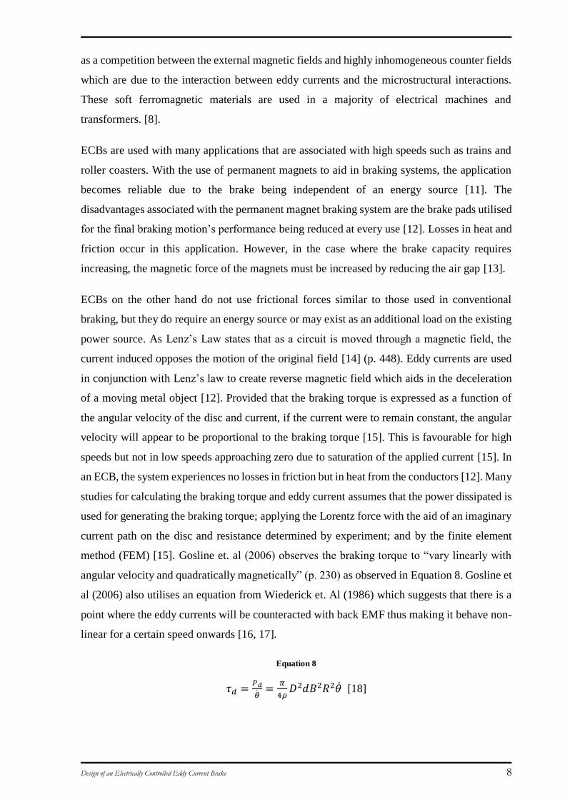
Caldwell and Taylor (1998) utilises Wouterse’s journal to explain Figure 5. In the operation of

an ECB, Gosline et. al (2006) also observed the behaviour in Figure 4 as did Caldwell and

Taylor (1998). Their observations include that the torque tends to vary linearly with the speed

as mentioned previously, however, the magnetic flux created for the disc is counteracted at

speeds greater than the critical speed. At speeds greater than the critical speed, Back EMF

reduces the torque achieved [19]. This is observed by the non-linear behaviour after

approximately 100 RPM in Figure 5. Gosline et al (2006) also assumes that in order to obtain

a linear relationship between torque and speed, the conductive disc must be within the cross

sectional area of the air gap. Thus, when the speed is below the critical speed and the conductive

disc is within the cross-sectional air gap area, a linear torque and speed relationship occurs.

Figure 5 Mathcad Model torque/speed curve, final design, 10 A coil current [19]

Design of an Electrically Controlled Eddy Current Brake 10

In theory, the breaking torque of the ECB can be expressed as a function of speed, torque and

current [15]. An ECB may be required to be used in conjunction with other conventional brake

systems due to the uncontrollable behaviour at low speeds [15].The drawback of this system is

that it is difficult to implement the brake at low speeds as the eddy currents oppose the field

proportionally and perpendicularly due to the relationship established by Equation 10 [20].

Equation 10 [20]

𝐸 = 𝑣 𝑥 𝐵

Observations from journals suggest that for different speeds in the air gap magnetic field, the

following applies:

At low speeds, the magnetic induction B is less than the 𝐵0 generated at zero speed

and therefore, theoretically, the magnetic induction B will be almost perpendicular

to the disc

At the critical speed region, where the braking force is a maximum, the average

induction under the pole of the electromagnet is significantly lower than 𝐵0 due to

the magnetic induction caused from the eddy being no longer comparable with 𝐵0

And finally, at high speeds, the magnetic induction decreases to the point where the

eddy currents cancels the magnetic field at infinite speeds

[20]

Karakoc (2012) suggests that if a soft magnetic core is used for an ECB, a field will be induced

in the core itself. Consequently, this results in non-linear relationships between the torque and

speed [6]. Karakoc (2012) also suggests that for low speeds, the rotational effects are dominant

over the induction effects. This is present in Karakoc’s (2012) small-scale model and FEM

results.

2.3.1 Models

There have been three major models that have been used and developed for eddy current braking

systems. The three models are Wouterse, Smythe and Schieber. These are reviewed in detail

below.

Wouterse’s model stems from Rudenberg’s ECB. Rudenberg designed a brake which would be

energised by direct current. Furthermore, Rudenberg made the assumption that the poles were

situated near each other in order to model the current and magnetic field via sinusoidal

functions. As mentioned in 2.3, heat is one of the foremost problems associated with ECBs.

Design of an Electrically Controlled Eddy Current Brake 11

Due to materials available today for the construction of the ECB, it has led to heat problems in

the disc due to power densities within the materials used. This has resulted in the requirement

for cooling techniques and wider spacing of the poles. As the ECB is a machine, the

mechanically absorbed power is dispersed by the disc. [21]

Smythe continued Rudenberg’s works investigating the current distribution surrounding the

pole on the disc. Smythe was successful in determining a relationship in the low speed region

but not for high speeds. [21]

Additionally, Schieber came to the same conclusion as Smythe but did not explore the high

speed region. Instead, the relationship for a linearly moving strip was determined. [21]

Many of those mentioned above found similar conclusions where the torque behaviour at high

speeds was asymptotic. Wouterse puts forth that if the pole is surrounded by a conducting slip

ring, it theoretically provides no resistance in the return path for the currents. In turn, this would

satisfy Smythe and Schieber’s theory regarding current patterns present in the disc. Wouterse

came to the conclusion that for low speeds, the drag force is proportional to speed however,

Wouterse found the existence of the resistance in the return path. [21]

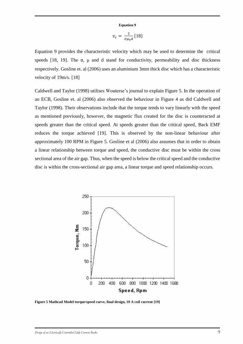
Smythe’s analysis in regards to the impact of eddy currents on a rotating disc states that the

method is accurate for permanent magnets. For electromagnets, the analysis is complicated due

to the permeable materials used in the poles creating a demagnetizing flux through the

electromagnet. Smythe (1942) utilises Maxwell’s second equation to calculate the relationship

between magnetic induction and an eddy current. Figure 6 shows the flow of eddy currents of

two magnets where the magnetic fields are parallel and have a radius of 100mm. [2]

Figure 6 Lines of Flow of Eddy Currents induced in rotating disc by two circular pole magnets [2]

Design of an Electrically Controlled Eddy Current Brake 12

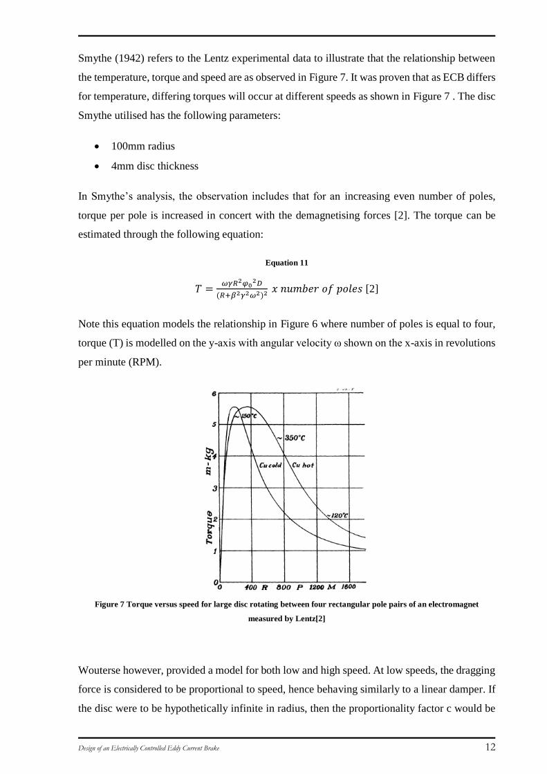
Smythe (1942) refers to the Lentz experimental data to illustrate that the relationship between

the temperature, torque and speed are as observed in Figure 7. It was proven that as ECB differs

for temperature, differing torques will occur at different speeds as shown in Figure 7 . The disc

Smythe utilised has the following parameters:

100mm radius

4mm disc thickness

In Smythe’s analysis, the observation includes that for an increasing even number of poles,

torque per pole is increased in concert with the demagnetising forces [2]. The torque can be

estimated through the following equation:

Equation 11

𝑇 =𝜔𝛾𝑅2𝜑0

2𝐷

(𝑅+𝛽2𝛾2𝜔2)2 𝑥 𝑛𝑢𝑚𝑏𝑒𝑟 𝑜𝑓 𝑝𝑜𝑙𝑒𝑠 [2]

Note this equation models the relationship in Figure 6 where number of poles is equal to four,

torque (T) is modelled on the y-axis with angular velocity ω shown on the x-axis in revolutions

per minute (RPM).

Figure 7 Torque versus speed for large disc rotating between four rectangular pole pairs of an electromagnet

measured by Lentz[2]

Wouterse however, provided a model for both low and high speed. At low speeds, the dragging

force is considered to be proportional to speed, hence behaving similarly to a linear damper. If

the disc were to be hypothetically infinite in radius, then the proportionality factor c would be

Design of an Electrically Controlled Eddy Current Brake 13

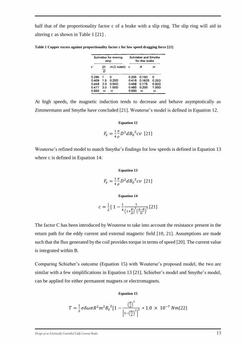
half that of the proportionality factor c of a brake with a slip ring. The slip ring will aid in

altering c as shown in Table 1 [21] .

Table 1 Copper excess against proportionality factor c for low speed dragging force [21]

At high speeds, the magnetic induction tends to decrease and behave asymptotically as

Zimmermann and Smythe have concluded [21]. Wouterse’s model is defined in Equation 12.

Equation 12

𝐹𝑒 =1

4

𝜋

𝜌𝐷2𝑑𝐵0

2𝑐𝑣 [21]

Wouterse’s refined model to match Smythe’s findings for low speeds is defined in Equation 13

where c is defined in Equation 14:

Equation 13

𝐹𝑒 =1

4

𝜋

𝜌𝐷2𝑑𝐵0

2𝑐𝑣 [21]

Equation 14

𝑐 =1

2[ 1 −

1

4

1

(1+𝑅

𝐴)2(𝐴−𝑅

𝐷)2 [21]

The factor C has been introduced by Wouterse to take into account the resistance present in the

return path for the eddy current and external magnetic field [10, 21]. Assumptions are made

such that the flux generated by the coil provides torque in terms of speed [20]. The current value

is integrated within B.

Comparing Schieber’s outcome (Equation 15) with Wouterse’s proposed model, the two are

similar with a few simplifications in Equation 13 [21]. Schieber’s model and Smythe’s model,

can be applied for either permanent magnets or electromagnets.

Equation 15

𝑇 =1

2𝜎𝛿𝜔𝜋𝑅2𝑚2𝐵𝑧

2[1 −(𝑅

𝑎)2

[1−(m

a)2]2 ∗ 1.0 × 10−7 𝑁𝑚[22]

Design of an Electrically Controlled Eddy Current Brake 14

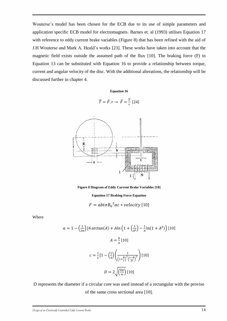
Wouterse’s model has been chosen for the ECB due to its use of simple parameters and

application specific ECB model for electromagnets. Barnes et. al (1993) utilises Equation 17

with reference to eddy current brake variables (Figure 8) that has been refined with the aid of

J.H Wouterse and Mark A. Heald’s works [23]. These works have taken into account that the

magnetic field exists outside the assumed path of the flux [10]. The braking force (F) in

Equation 13 can be substituted with Equation 16 to provide a relationship between torque,

current and angular velocity of the disc. With the additional alterations, the relationship will be

discussed further in chapter 4.

Equation 16

�⃗� = 𝐹 . 𝑟 → 𝐹 =�⃗�

𝑟 [24]

Figure 8 Diagram of Eddy Current Brake Variables [10]

Equation 17 Braking Force Equation

𝐹 = 𝑎𝑏𝑡𝜎𝐵02𝛼𝑐 ∗ 𝑣𝑒𝑙𝑜𝑐𝑖𝑡𝑦 [10]

Where

𝛼 = 1 − (1

2𝜋) [4 arctan(𝐴) + 𝐴𝑙𝑛 (1 + (

1

𝐴2) −1

𝐴ln(1 + 𝐴2)) [10]

𝐴 =𝑏

𝑎 [10]

𝑐 =1

2[1 − (

1

4)(

1

(1+𝑅

𝑟)2(𝑟−𝑅

𝐷)2 ) [10]

𝐷 = 2√(𝑏𝑎

𝜋) [10]

D represents the diameter if a circular core was used instead of a rectangular with the proviso

of the same cross sectional area [10].

Design of an Electrically Controlled Eddy Current Brake 15

2.4 Finite Element Analysis (FEA)

In engineering applications, the state variables of an eddy current can be described with partial

differential equations with other parameters that link the input mechanical power and angular

speed response. This must include the known variables such as conductive disc dimensions and

the air gap distance. However, the non-linear relationships between these variables become

complex and impossible to calculate over numerous iterations and therefore, require another

method other than analytical. Finite Element Analysis (FEA) on the other hand, can solve these

iterative equations and is used today to solve static and dynamic problems including fluid

mechanics and electromagnetics. [25]

In conducting an FEA for an ECB, the following considerations must be made:

Analysis as either Two-Dimensional (2D) or Three-Dimensional (3D)

Method as either transport-term or transient

Boundary conditions

Periodicities and symmetries

Level of approximation of the properties of the material

The difference between a 2D and 3D analysis is that a 3D analysis requires a strong processor

and requires a longer time to simulate. A 2D analysis is easier and quicker than a 3D but is

disadvantaged of not accepting 3D boundary condition parameters, hence approximations must

be made in order to make the model accurate. [26]

The methods which are applicable to ECBs are transport-term and transient methods. The

transport-term method consists of adding a conductivity and velocity term to the analysis. This

is ideal for a simple ECB which does not consist of cooling fins or holes. A transient method

begins with the disc at rest before bringing it to the desired speed. However, it will have to

undergo several trials in order to observe the transients occurring. As mentioned, this method

is time consuming due to the need of computing several trials for every transient that occurs

and the complexity of the equations. [26]

Finite Element Method (FEM) is an accurate way of predicting the model as well as confirming

the behaviour of the eddy current and the interaction of the flux density [27]. However, for train

applications, many journals have also conducted a 3D analysis in order to take into account flux

distribution [27]. In an ECB, there are finite element equations which are used for areas that are

conducting and non-conducting. For non-conducting areas, Equation 18 is used. In conducting

areas such as the eddy current paths, Equation 19 is used. [24]

Design of an Electrically Controlled Eddy Current Brake 16

Equation 18

𝐸 = −𝜕𝐴

𝜕𝑡− ∇. 𝑉 + 𝜔 𝑥 ∇ 𝑥 𝐴 [24]

Equation 19

∇ 𝑥1

𝜇𝑥∇𝑥𝐴 = 𝜎 (−

𝜕𝐴

𝜕𝑡− (𝜔. ∇)𝐴 − (𝐴. ∇)𝜔 − 𝐴𝑥(∇𝑥𝜔)) [24]

Where:

V= scalar electric potential

ω = speed

A = magnetic potential field which is defined along the electrical potential φ [28]

Through a 3D transient magnetic model, the simulation is able to produce the relationship

between torque, speed and current. Not only can that relationship be confirmed through a 3D

analysis, the interaction between the eddy current and conductive disc can also be shown. [24]

Gulbahce’s (2013) journal article titled “A study to determine the excitation current of the

braking torque of a low Eddy Current Brake” states that the conductive material exposed to the

current can be expressed as Equation 20 [24]. Gulbahce (2013) found that as the current varies,

the critical speed remains constant [24]. This agrees with Lentz’s measurements for torque and

speed in Smythe’s journal article mentioned previously.

Equation 20

∇𝑥�⃗� = −𝜕�⃗�

𝜕𝑡 [24]

Gay and Ehsani (2006) states that the use of FEM is to model the properties of the ferromagnetic

material in the brake and therefore, be able to observe the brake’s performance. It is also

mentioned that the ferromagnetic materials that are used for ECBs have the same properties due

to the process of casting [26].

Design of an Electrically Controlled Eddy Current Brake 17

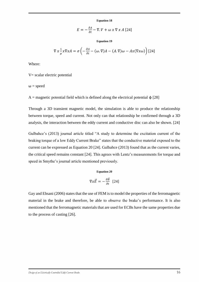
3 Determination of Magnetisation Curve

In order to understand the relationship between the flux density (B) and flux intensity (H) within

a core, the magnetisation curve is determined. This experiment allows for an accurate analysis

of the material’s properties in terms of flux density and field intensity. From this point, the

predicted torque at various speeds can be determined through Matlab to produce Figure 9.

Through this experiment, the saturation point will also be determined which is also known as

the limit of the maximum achievable magnetic flux density in the material [29].

Aim: Determine the Magnetisation Curve

Method:

Firstly, the theoretical number of turns, current and voltage was calculated with the following

equations:

𝐻(𝑡) =𝑁𝑀𝑎𝑖𝑛𝑖𝑀𝑎𝑖𝑛(𝑡)

𝑙𝑐𝑜𝑟𝑒 (i)

𝑉𝑆 = 4.44𝑁𝑀𝑎𝑖𝑛𝐵𝑝𝑘𝐴𝑐𝑜𝑟𝑒𝑓 (ii)

𝐵(𝑡) =1

𝐴𝑐𝑜𝑟𝑒𝑁𝑀𝑎𝑖𝑛∫ 𝑣𝑠𝑒𝑛𝑠𝑒𝑑𝑡 =

1

𝐴𝑐𝑜𝑟𝑒𝑁𝑀𝑎𝑖𝑛𝜆𝑠𝑒𝑛𝑠𝑒(𝑡) (iii)

𝜆𝑠𝑒𝑛𝑠𝑒[𝑘 + 1] = 𝜆𝑠𝑒𝑛𝑠𝑒[𝑘] + 𝑣𝑆𝑒𝑛𝑠𝑒[𝑘]∆𝑡 (iv)

[29]

These equations were solved with Matlab with the known parameters:

f=50Hz

L(core)=0.4791 m

Bpk=2.5T

H(core)=2500At/m

According to Figure 9, the number of turns should be 144 for the maximum current of 10A. It

was observed however, that with 144 turns, the current was still not being passed. 44 turns were

taken off the primary turns in order for the current to flow. The secondary turns otherwise

known as the sensing coil used a thinner wire with fewer turns, in this experiment, 15 turns.

Design of an Electrically Controlled Eddy Current Brake 18

Figure 9 Relationship between voltage, current and number of turns

0 100 200 300 400 500 600 7000

100

200

300

400

500

600

Current

voltage(V

) N

main

(turn

s)

X: 10.01Y: 65

X: 10.01Y: 143.5

Voltage vs. Current

Nmain vs. Current

Design of an Electrically Controlled Eddy Current Brake 19

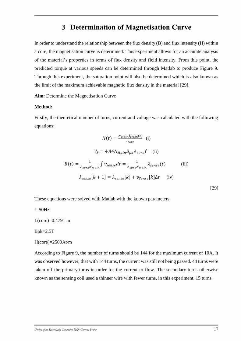
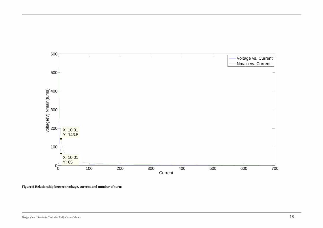
Figure 10 and Figure 11 demonstrates the general setup of the experiment. The range of currents

that were utilised ranged between 0.078A to 10A.

Figure 10 Magnetisation Curve Set up [29]

Figure 11 Experimental set up

The measurements required from the oscilloscope is the current in the primary turns and the

voltage measured in the sensing coil. The sensing coil is used to measure the magnetic flux

density induced by the primary windings [29].

After obtaining the measurements, the DC offsets are required to be removed by calculating the

mean of both signals and subtracting them from their respectful signals. The flux was calculated

via (i). The flux linkage can be determined by using (iii and iv) and removing the DC offset.

The final step is to plot the BH values to obtain the hysteresis curve. The magnetisation curve

is determined by plotting the peak values of B and H.

Design of an Electrically Controlled Eddy Current Brake 20

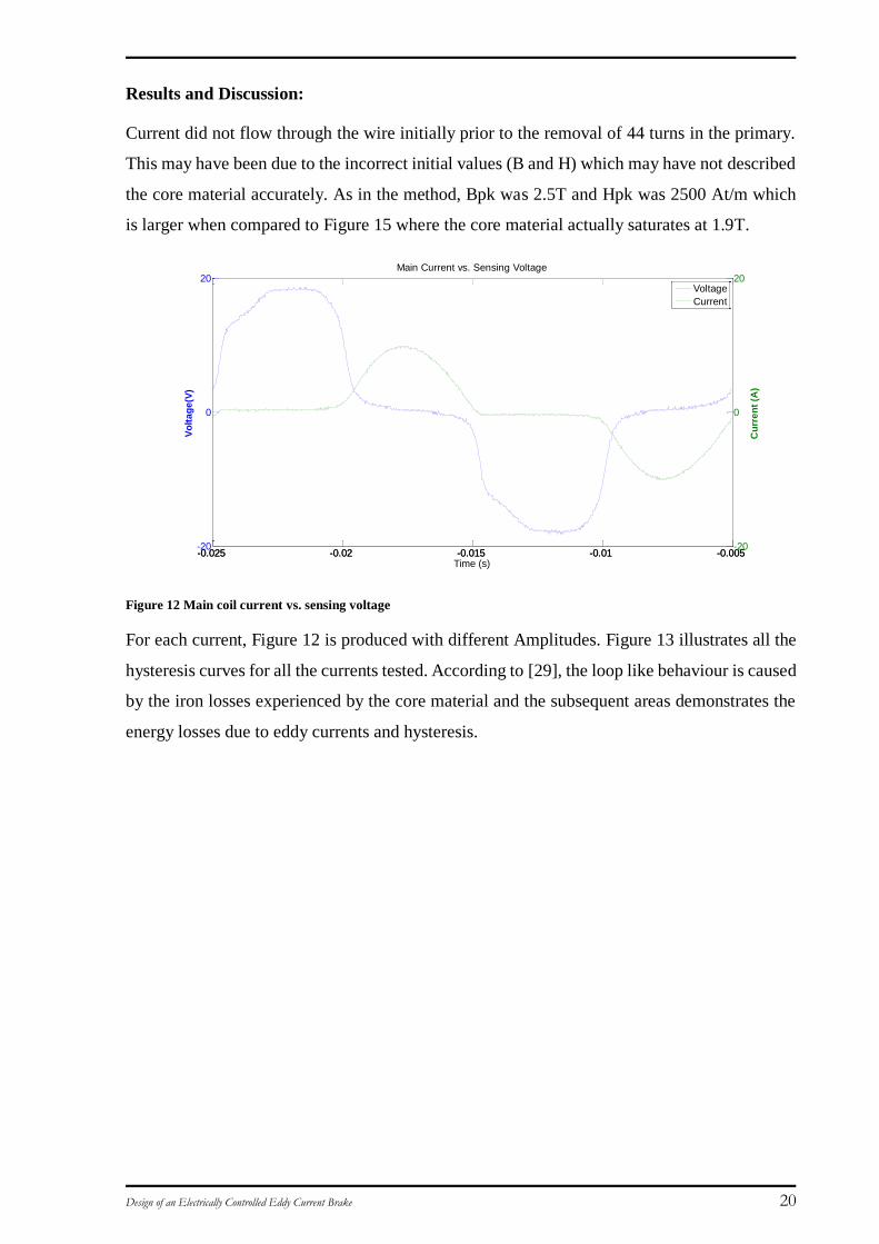
Results and Discussion:

Current did not flow through the wire initially prior to the removal of 44 turns in the primary.

This may have been due to the incorrect initial values (B and H) which may have not described

the core material accurately. As in the method, Bpk was 2.5T and Hpk was 2500 At/m which

is larger when compared to Figure 15 where the core material actually saturates at 1.9T.

Figure 12 Main coil current vs. sensing voltage

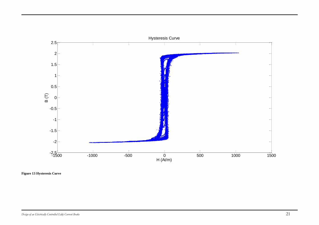
For each current, Figure 12 is produced with different Amplitudes. Figure 13 illustrates all the

hysteresis curves for all the currents tested. According to [29], the loop like behaviour is caused

by the iron losses experienced by the core material and the subsequent areas demonstrates the

energy losses due to eddy currents and hysteresis.

-0.025 -0.02 -0.015 -0.01 -0.005-20

0

20

Vo

lta

ge

(V)

Time (s)

Main Current vs. Sensing Voltage

-0.025 -0.02 -0.015 -0.01 -0.005-20

0

20

Cu

rre

nt

(A)

Voltage

Current

Design of an Electrically Controlled Eddy Current Brake 21

Figure 13 Hysteresis Curve

-1500 -1000 -500 0 500 1000 1500-2.5

-2

-1.5

-1

-0.5

0

0.5

1

1.5

2

2.5Hysteresis Curve

H (At/m)

B (

T)

Design of an Electrically Controlled Eddy Current Brake 22

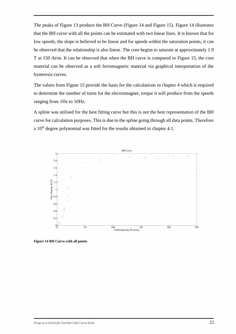
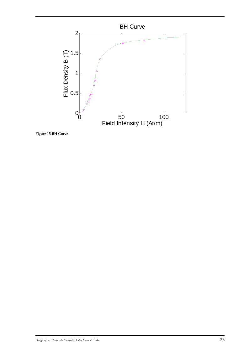
The peaks of Figure 13 produce the BH Curve (Figure 14 and Figure 15). Figure 14 illustrates

that the BH curve with all the points can be estimated with two linear lines. It is known that for

low speeds, the slope is believed to be linear and for speeds within the saturation points, it can

be observed that the relationship is also linear. The core begins to saturate at approximately 1.9

T at 150 At/m. It can be observed that when the BH curve is compared to Figure 15, the core

material can be observed as a soft ferromagnetic material via graphical interpretation of the

hysteresis curves.

The values from Figure 15 provide the basis for the calculations in chapter 4 which is required

to determine the number of turns for the electromagnet, torque it will produce from the speeds

ranging from 1Hz to 10Hz.

A spline was utilised for the best fitting curve but this is not the best representation of the BH

curve for calculation purposes. This is due to the spline going through all data points. Therefore

a 10th degree polynomial was fitted for the results obtained in chapter 4.1.

Figure 14 BH Curve with all points

0 50 100 150 200 2500

0.2

0.4

0.6

0.8

1

1.2

1.4

1.6

1.8

2BH Curve

Field Intensity H (At/m)

Flu

x D

ensi

ty B

(T

)

Design of an Electrically Controlled Eddy Current Brake 23

Figure 15 BH Curve

0 50 1000

0.5

1

1.5

2BH Curve

Field Intensity H (At/m)

Flu

x D

ensity B

(T

)

Design of an Electrically Controlled Eddy Current Brake 24

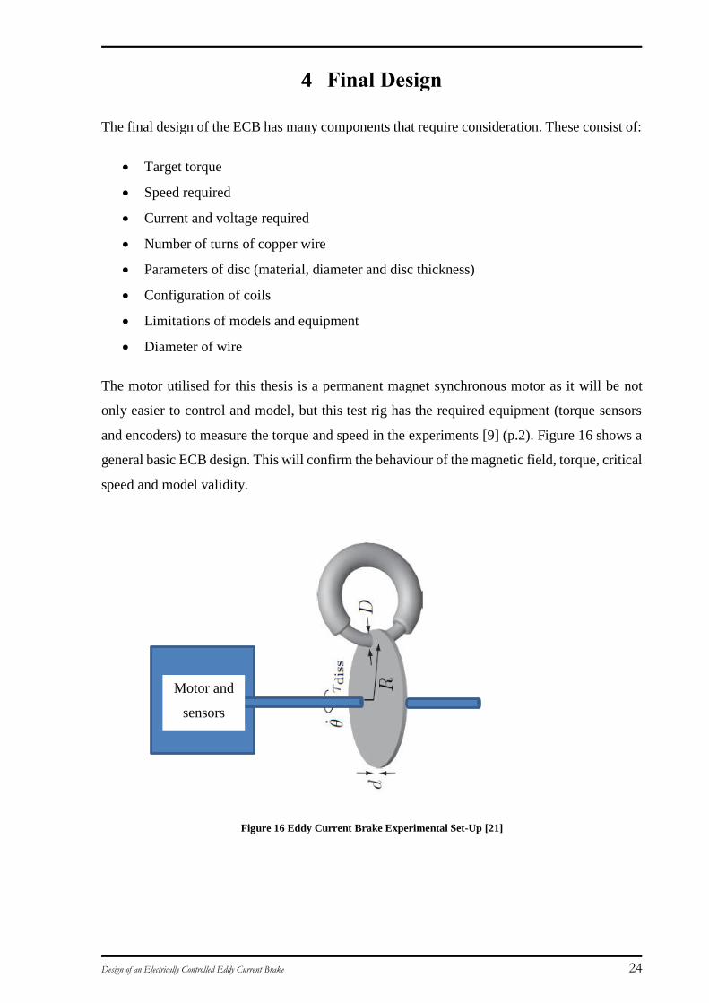
4 Final Design

The final design of the ECB has many components that require consideration. These consist of:

Target torque

Speed required

Current and voltage required

Number of turns of copper wire

Parameters of disc (material, diameter and disc thickness)

Configuration of coils

Limitations of models and equipment

Diameter of wire

The motor utilised for this thesis is a permanent magnet synchronous motor as it will be not

only easier to control and model, but this test rig has the required equipment (torque sensors

and encoders) to measure the torque and speed in the experiments [9] (p.2). Figure 16 shows a

general basic ECB design. This will confirm the behaviour of the magnetic field, torque, critical

speed and model validity.

Figure 16 Eddy Current Brake Experimental Set-Up [21]

Motor and

sensors

Design of an Electrically Controlled Eddy Current Brake 25

4.1 Calculations:

The calculation for the corresponding flux density used in Wouterse’s model are from the

magnetisation curve determined in Chapter 3. As mentioned in 1.2, this electromagnet must

achieve a torque of at least 0.3Nm and a maximum speed of 10Hz.

In conducting calculations, the value of B and its corresponding H value were initially used to

determine the parameters of the ECB and torque using Matlab. Equations from Sen (1997) were

used for this procedure [5]. The equations used are as follows:

𝐵 = 𝜇0𝜇𝑟𝐻

𝐹𝑐 = 𝐻𝑐𝑙𝑐

𝐹𝑔 = 𝐻𝑔𝑙𝑔 → 𝐹𝑔 = 𝐻𝑐𝑙𝑔 (if air gap is relatively small in comparison to the mean core length)

𝐹𝑇 = 𝐹𝑐 + 𝐹𝑔

𝐹𝑇 = 𝑁𝑖 → 𝑖 =𝐹𝑇

𝑁

[5]

The above equations were utilised to determine the current required to force the flux through

the electromagnet. There are many alternatives that were considered for completing the flux

path. These consist of:

a) Using a set-up similar to Appendix C: Proposed Design. By having a backing plate’s

thickness greater than the rod’s diameter, the reluctance for the backing plate can be

neglected in comparison to the rod’s reluctance. An FEA analysis can confirm the

behaviour of magnetic flux.

b) Using a toroidal core where a slit is required to be cut for the air gap

c) Using a square core with similar actions required from b)

This thesis uses a toroidal core as observed in Figure 16 and as mentioned in chapter 1.2, an

Axial Flux PMSM motor to provide the load.

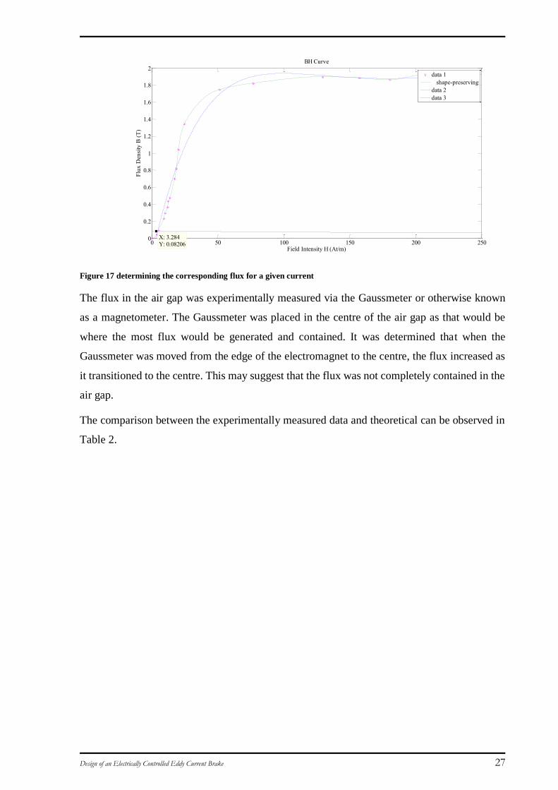
4.1.1 Corresponding Flux Density used in Torque Calculations

This resulting load line and corresponding flux density for 0.5A is illustrated in Figure 17. It

was observed that for currents below 0.5A, the curve fitting methods provide different results.

Design of an Electrically Controlled Eddy Current Brake 26

For instance, the green curve is a shape preserving curve. This is closer to the BH curve

observed in Figure 3. The blue curve is fitted by a 10th degree polynomial. The issue with using

polynomials is that it does not necessary intersect at the origin.

The corresponding flux density utilised for a given current was calculated by determining the

load line. The parameters include:

𝑁𝑖 = 𝐻𝑔𝐿𝑔 + 𝐻𝑐𝐿𝐶 =𝐵𝑔

𝜇0𝐿𝑔 + 𝐻𝑐𝐿𝑐

Where:

Hg = field intensity of air gap (At/m),

Hc = field intensity of core (At/m),

µ0 = permeability of free space (4πe-7 h/m),

Lc = mean length of core (m),

Lg = length of air gap (m)

𝐵𝑔 = 𝐵𝑐 = −𝜇0 (𝐿𝑐

𝐿𝑔)𝐻𝑐 +

𝑁𝑖𝜇0

𝐿𝑔

Where:

Bg = Bc = flux density of core/air gap (assuming no leakage flux)

This is in the form of the linear equation y=mx+c, this is known as the load line and is plotted

on the BH Curve.

𝑚 = 𝐻𝑐 = −𝜇0 (𝐿𝑐

𝐿𝑔)

The B intersection point is:

𝑐 = 𝐵𝑔 =𝑁𝑖𝜇0

𝐿𝑔

[5]

The resulting load line is observed in Figure 17 for 0.5A. The flux density obtained for 0.5A is

0.08206 T.

Design of an Electrically Controlled Eddy Current Brake 27

Figure 17 determining the corresponding flux for a given current

The flux in the air gap was experimentally measured via the Gaussmeter or otherwise known

as a magnetometer. The Gaussmeter was placed in the centre of the air gap as that would be

where the most flux would be generated and contained. It was determined that when the

Gaussmeter was moved from the edge of the electromagnet to the centre, the flux increased as

it transitioned to the centre. This may suggest that the flux was not completely contained in the

air gap.

The comparison between the experimentally measured data and theoretical can be observed in

Table 2.

0 50 100 150 200 2500

0.2

0.4

0.6

0.8

1

1.2

1.4

1.6

1.8

2

BH Curve

Field Intensity H (At/m)

Flu

x D

ensi

ty B

(T

)

X: 3.284Y: 0.08206

data 1

shape-preserving

data 2

data 3

Design of an Electrically Controlled Eddy Current Brake 28

Table 2 Comparison of Flux Density Values

Current 0.1 0.2 0.3 0.4 0.5 1 2 3 4 5

1st Linear 0.01636 0.03282 0.04928 0.06578 0.08231 0.1646 0.3292 0.4938 0.6584 0.8231

Spline 0.01623 0.03266 0.04909 0.06558 0.08198 0.1641 0.3286 0.4929 0.6572 0.8223

10th Order Polynomial 0.0162 0.03263 0.04909 0.06552 0.08198 0.164 0.3286 0.4929 0.6578 0.8214

% diff 0.988% 0.582% 0.387% 0.397% 0.403% 0.366% 0.183% 0.183% 0.091% 0.207%

Experimentally measured trial 1

0.01682 0.03344 0.04918 0.06708 0.08399 0.161163 0.32 0.4726 0.5352 0.56255

Experimentally measured trial 2

0.01683 0.03343 0.04918 0.06708 0.0839 0.169427 0.336133 0.499266667 0.571467 0.6062

Average between experiment data 0.01682 0.03344 0.04918 0.06708 0.083945 0.165295 0.328067 0.485933333 0.553333 0.584375

% diff (between experiment only) 0.059% 0.030% 0.000% 0.000% 0.107% 4.877% 4.800% 5.341% 6.346% 7.201%

%diff (experiment and theory) 3.686% 2.422% 0.183% 2.326% 2.393% 1.760% 2.688% 4.295% 22.907% 46.014%

Design of an Electrically Controlled Eddy Current Brake 29

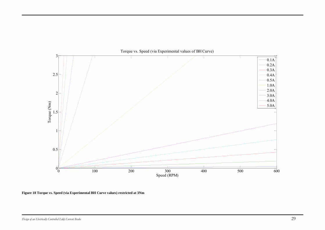
Figure 18 Torque vs. Speed (via Experimental BH Curve values) restricted at 3Nm

0 100 200 300 400 500 6000

0.5

1

1.5

2

2.5

3Torque vs. Speed (via Experimental values of BH Curve)

Speed (RPM)

To

rqu

e (N

m)

0.1A

0.2A

0.3A

0.4A

0.5A

1.0A

2.0A

3.0A

4.0A

5.0A

Design of an Electrically Controlled Eddy Current Brake 30

Figure 18 demonstrates the theoretical relationship between torque, speed and current. It

exhibits that for a given current, certain torques and speeds can be achieved. Each line in Figure

18 represents a current with the top line representing the highest current, 5A. It can be observed

that for a given current, the corresponding flux determined earlier will in turn affect the torque

obtained at various speeds. The experimental limitations will affect the achievable torques as

the highest current (~5A) exceeds the 2.5Nm limit of the motor and achieves less than 1Hz at

lower speeds. The disadvantage of an ECB is that as the speed of the disc decreases, so does

the EMF produced by the applied current. Therefore, it will not be an effective brake at very

low speeds.

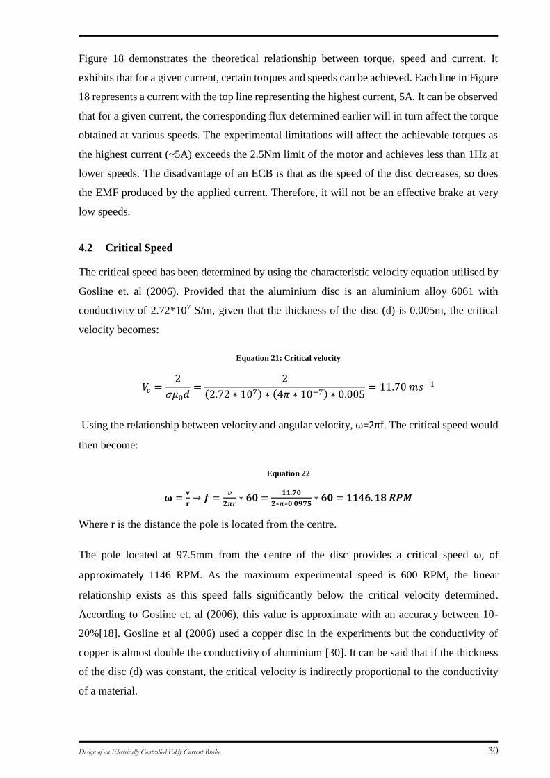
4.2 Critical Speed

The critical speed has been determined by using the characteristic velocity equation utilised by

Gosline et. al (2006). Provided that the aluminium disc is an aluminium alloy 6061 with

conductivity of 2.72*107 S/m, given that the thickness of the disc (d) is 0.005m, the critical

velocity becomes:

Equation 21: Critical velocity

𝑉𝑐 =2

𝜎𝜇0𝑑=

2

(2.72 ∗ 107) ∗ (4𝜋 ∗ 10−7) ∗ 0.005= 11.70 𝑚𝑠−1

Using the relationship between velocity and angular velocity, ω=2πf. The critical speed would

then become:

Equation 22

𝛚 =𝐯

𝐫→ 𝒇 =

𝒗

𝟐𝝅𝒓∗ 𝟔𝟎 =

𝟏𝟏.𝟕𝟎

𝟐∗𝝅∗𝟎.𝟎𝟗𝟕𝟓∗ 𝟔𝟎 = 𝟏𝟏𝟒𝟔. 𝟏𝟖 𝑹𝑷𝑴

Where r is the distance the pole is located from the centre.

The pole located at 97.5mm from the centre of the disc provides a critical speed ω, of

approximately 1146 RPM. As the maximum experimental speed is 600 RPM, the linear

relationship exists as this speed falls significantly below the critical velocity determined.

According to Gosline et. al (2006), this value is approximate with an accuracy between 10-

20%[18]. Gosline et al (2006) used a copper disc in the experiments but the conductivity of

copper is almost double the conductivity of aluminium [30]. It can be said that if the thickness

of the disc (d) was constant, the critical velocity is indirectly proportional to the conductivity

of a material.

Design of an Electrically Controlled Eddy Current Brake 31

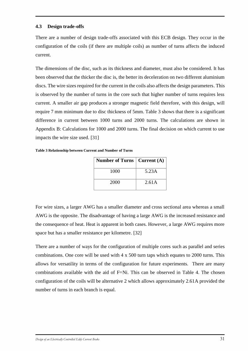
4.3 Design trade-offs

There are a number of design trade-offs associated with this ECB design. They occur in the

configuration of the coils (if there are multiple coils) as number of turns affects the induced

current.

The dimensions of the disc, such as its thickness and diameter, must also be considered. It has

been observed that the thicker the disc is, the better its deceleration on two different aluminium

discs. The wire sizes required for the current in the coils also affects the design parameters. This

is observed by the number of turns in the core such that higher number of turns requires less

current. A smaller air gap produces a stronger magnetic field therefore, with this design, will

require 7 mm minimum due to disc thickness of 5mm. Table 3 shows that there is a significant

difference in current between 1000 turns and 2000 turns. The calculations are shown in

Appendix B: Calculations for 1000 and 2000 turns. The final decision on which current to use

impacts the wire size used. [31]

Table 3 Relationship between Current and Number of Turns

Number of Turns Current (A)

1000 5.23A

2000 2.61A

For wire sizes, a larger AWG has a smaller diameter and cross sectional area whereas a small

AWG is the opposite. The disadvantage of having a large AWG is the increased resistance and

the consequence of heat. Heat is apparent in both cases. However, a large AWG requires more

space but has a smaller resistance per kilometre. [32]

There are a number of ways for the configuration of multiple cores such as parallel and series

combinations. One core will be used with 4 x 500 turn taps which equates to 2000 turns. This

allows for versatility in terms of the configuration for future experiments. There are many

combinations available with the aid of F=Ni. This can be observed in Table 4. The chosen

configuration of the coils will be alternative 2 which allows approximately 2.61A provided the

number of turns in each branch is equal.

Design of an Electrically Controlled Eddy Current Brake 32

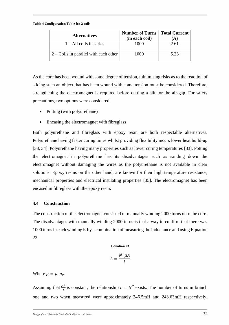
Table 4 Configuration Table for 2 coils

Alternatives Number of Turns

(in each coil)

Total Current

(A)

1 – All coils in series 1000 2.61

2 – Coils in parallel with each other 1000 5.23

As the core has been wound with some degree of tension, minimising risks as to the reaction of

slicing such an object that has been wound with some tension must be considered. Therefore,

strengthening the electromagnet is required before cutting a slit for the air-gap. For safety

precautions, two options were considered:

Potting (with polyurethane)

Encasing the electromagnet with fibreglass

Both polyurethane and fibreglass with epoxy resin are both respectable alternatives.

Polyurethane having faster curing times whilst providing flexibility incurs lower heat build-up

[33, 34]. Polyurethane having many properties such as lower curing temperatures [33]. Potting

the electromagnet in polyurethane has its disadvantages such as sanding down the

electromagnet without damaging the wires as the polyurethane is not available in clear

solutions. Epoxy resins on the other hand, are known for their high temperature resistance,

mechanical properties and electrical insulating properties [35]. The electromagnet has been

encased in fibreglass with the epoxy resin.

4.4 Construction

The construction of the electromagnet consisted of manually winding 2000 turns onto the core.

The disadvantages with manually winding 2000 turns is that a way to confirm that there was

1000 turns in each winding is by a combination of measuring the inductance and using Equation

23.

Equation 23

𝐿 =𝑁2𝜇𝐴

𝑙

Where 𝜇 = 𝜇0𝜇𝑟

Assuming that 𝜇𝐴

𝑙 is constant, the relationship 𝐿 = 𝑁2 exists. The number of turns in branch

one and two when measured were approximately 246.5mH and 243.63mH respectively.

Design of an Electrically Controlled Eddy Current Brake 33

Therefore, each branch holds approximately 1047 and 1051 turns respectively. As the two

branches are connected in parallel, the relationship of resistances in parallel cannot be applied.

The relationship becomes:

Equation 24

𝐿𝑛𝑒𝑤 = (2𝑁)2 = 4𝑁2 = 4𝐿

Equation 24 confirms the measured value of inductance when they are connected in parallel.

The value obtained is 452.7mH which confirms the value obtained from substituting L as the

average of the two inductances.

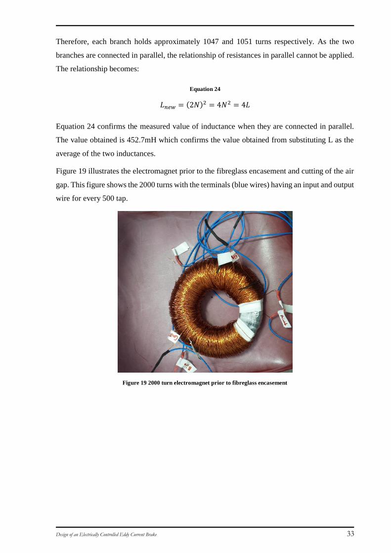
Figure 19 illustrates the electromagnet prior to the fibreglass encasement and cutting of the air

gap. This figure shows the 2000 turns with the terminals (blue wires) having an input and output

wire for every 500 tap.

Figure 19 2000 turn electromagnet prior to fibreglass encasement

Design of an Electrically Controlled Eddy Current Brake 34

Figure 20 Fibreglass encasement

4.5 Experimental Set-up

As Sen (1997) mentioned in chapter 2.1.2, an electromagnetic circuit can be used to conduct

calculations to determine the amount of current required to force the flux through the air gap.

The current design which is illustrated in Figure 21 has simpler calculations in comparison to

the preliminary design with it being a toroidal core with one air gap. The toroidal core is also

available in the market with the exception that the air gap will be required to be cut, therefore

reducing manufacturing costs. The new proposed design which will be presented in Appendix

C: Proposed Design would require the majority of the parts to be manufactured in order to

achieve the ideal ECB geometry parameters. The theoretical calculations for the new proposed

design will have a complicated set of calculations, however FEA analysis should be used for

the proposed design.

The final design consists of the following:

1 x toroidal core

5mm aluminium disc with 200mm diameter

Bearings and plywood

Fibreglass encasement of electromagnet

Wire size to be 0.064mm with 2000 turns. (with 500 taps)

For versatility, 500 turn taps will be included so that the electromagnet can be used with

different configurations.

Design of an Electrically Controlled Eddy Current Brake 35

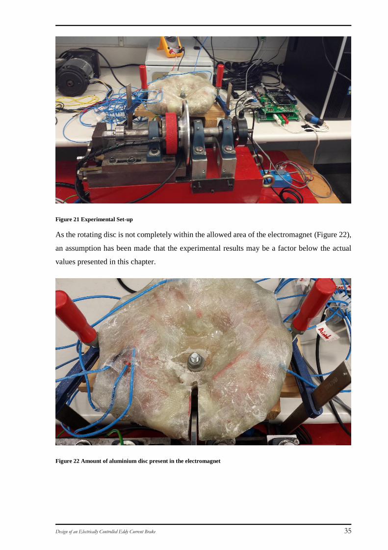
Figure 21 Experimental Set-up

As the rotating disc is not completely within the allowed area of the electromagnet (Figure 22),

an assumption has been made that the experimental results may be a factor below the actual

values presented in this chapter.

Figure 22 Amount of aluminium disc present in the electromagnet

Design of an Electrically Controlled Eddy Current Brake 36

5 Results

Chapter 2.3 discussed the models available for ECBs. It also detailed the critical parameters to

successfully develop an ECB.

This chapter will present the experimental comparison with the theoretical and experimentally

measured flux.

The measurement of the results were via a torque sensor and an encoder which measured the

speed in Hertz. The axial flux PMSM motor provided the load for the ECB.

5.1 Validity of assumptions

Chapters 2.1.2 and 2.3 presented the following assumptions:

For magnetic circuits:

Hysteresis and BH curve presented in chapter 3 is valid and correct

For ECB designs:

Magnetic flux is uniform in the air gap

Conductive disc fits exactly within the air-gap

Relationship between the torque and speed is linear provided it is below the critical

velocity

[16]

5.2 Eddy Current Brake Testing Results

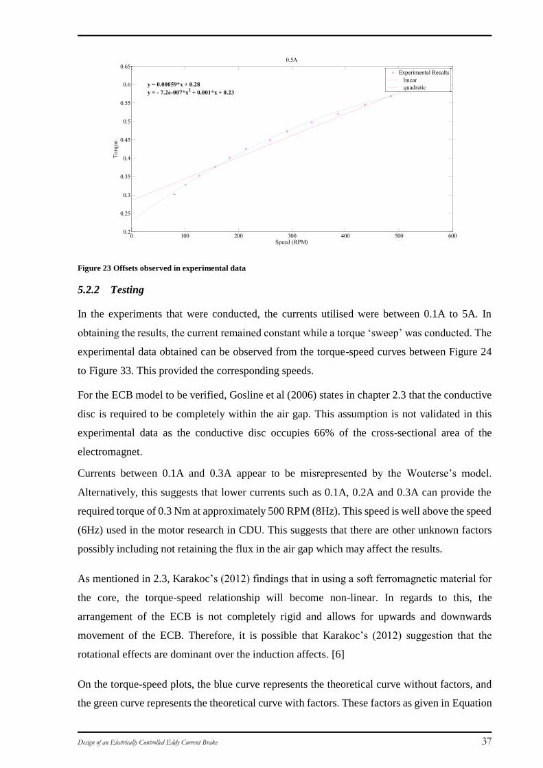
5.2.1 Torque Offset

In all the results that were obtained, there appeared to be an offset. Figure 23 provides an

example of this for a singular dataset. In order to minimise the amount of torque offset, the

torque sensor was reset to zero prior to every trial when data was collected. The torque offset

was determined by using the curve fitting tool in Matlab. The quadratic and linear function were

utilised to determine the offset as the correlation between the points. The quadratic offset value

was used in this case as it was a model where the relationship between the experimental data

had a better correlation. This method was applied to all the sets of torques obtained for the

corresponding currents.

Design of an Electrically Controlled Eddy Current Brake 37

Figure 23 Offsets observed in experimental data

5.2.2 Testing

In the experiments that were conducted, the currents utilised were between 0.1A to 5A. In

obtaining the results, the current remained constant while a torque ‘sweep’ was conducted. The

experimental data obtained can be observed from the torque-speed curves between Figure 24

to Figure 33. This provided the corresponding speeds.

For the ECB model to be verified, Gosline et al (2006) states in chapter 2.3 that the conductive

disc is required to be completely within the air gap. This assumption is not validated in this

experimental data as the conductive disc occupies 66% of the cross-sectional area of the

electromagnet.

Currents between 0.1A and 0.3A appear to be misrepresented by the Wouterse’s model.

Alternatively, this suggests that lower currents such as 0.1A, 0.2A and 0.3A can provide the

required torque of 0.3 Nm at approximately 500 RPM (8Hz). This speed is well above the speed

(6Hz) used in the motor research in CDU. This suggests that there are other unknown factors

possibly including not retaining the flux in the air gap which may affect the results.

As mentioned in 2.3, Karakoc’s (2012) findings that in using a soft ferromagnetic material for

the core, the torque-speed relationship will become non-linear. In regards to this, the

arrangement of the ECB is not completely rigid and allows for upwards and downwards

movement of the ECB. Therefore, it is possible that Karakoc’s (2012) suggestion that the

rotational effects are dominant over the induction affects. [6]

On the torque-speed plots, the blue curve represents the theoretical curve without factors, and

the green curve represents the theoretical curve with factors. These factors as given in Equation

0 100 200 300 400 500 6000.2

0.25

0.3

0.35

0.4

0.45

0.5

0.55

0.6

0.650.5A

Speed (RPM)

To

rqu

e

y = 0.00059*x + 0.28

y = - 7.2e-007*x2 + 0.001*x + 0.23

Experimental Results

linear

quadratic

Design of an Electrically Controlled Eddy Current Brake 38

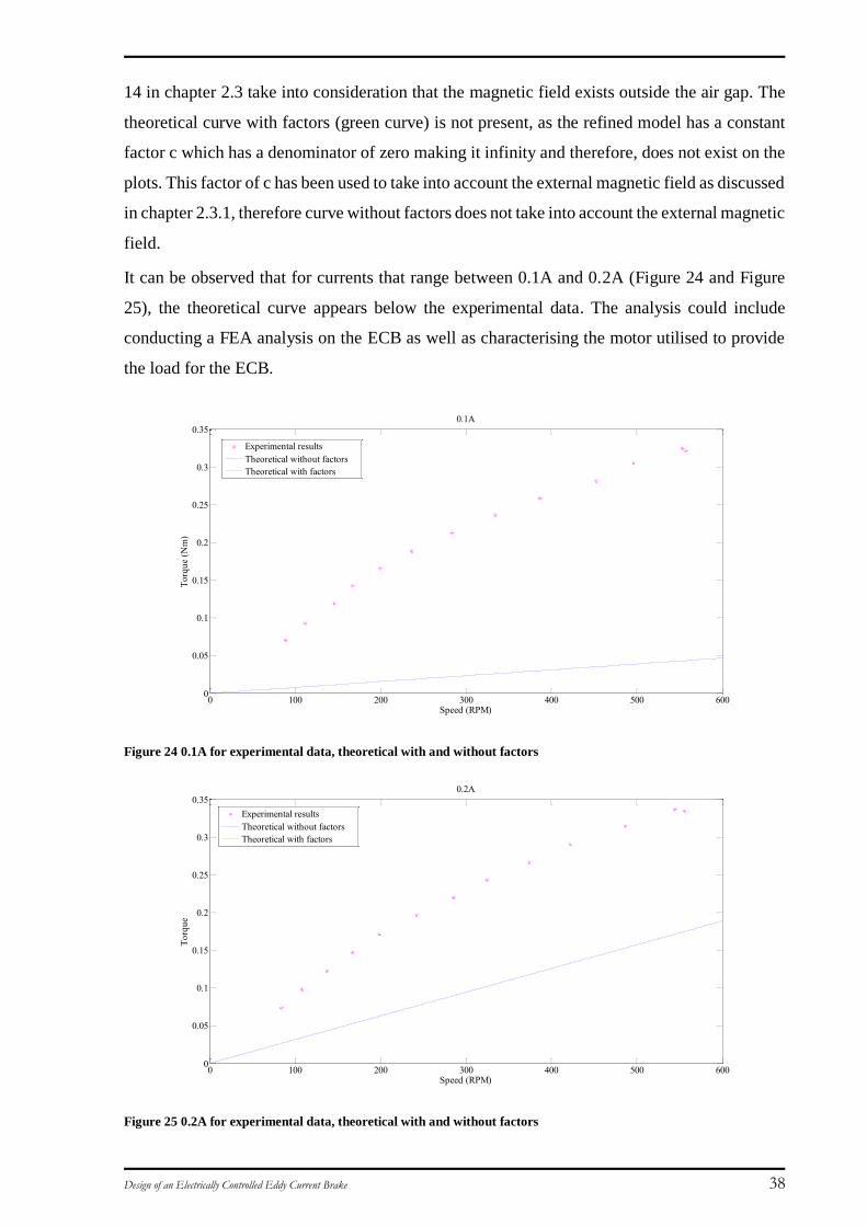
14 in chapter 2.3 take into consideration that the magnetic field exists outside the air gap. The

theoretical curve with factors (green curve) is not present, as the refined model has a constant

factor c which has a denominator of zero making it infinity and therefore, does not exist on the

plots. This factor of c has been used to take into account the external magnetic field as discussed

in chapter 2.3.1, therefore curve without factors does not take into account the external magnetic

field.

It can be observed that for currents that range between 0.1A and 0.2A (Figure 24 and Figure

25), the theoretical curve appears below the experimental data. The analysis could include

conducting a FEA analysis on the ECB as well as characterising the motor utilised to provide

the load for the ECB.

Figure 24 0.1A for experimental data, theoretical with and without factors

Figure 25 0.2A for experimental data, theoretical with and without factors

0 100 200 300 400 500 6000

0.05

0.1

0.15

0.2

0.25

0.3

0.350.1A

Speed (RPM)

To

rqu

e (N

m)

Experimental results

Theoretical without factors

Theoretical with factors

0 100 200 300 400 500 6000

0.05

0.1

0.15

0.2

0.25

0.3

0.350.2A

Speed (RPM)

To

rqu

e

Experimental results

Theoretical without factors

Theoretical with factors

Design of an Electrically Controlled Eddy Current Brake 39

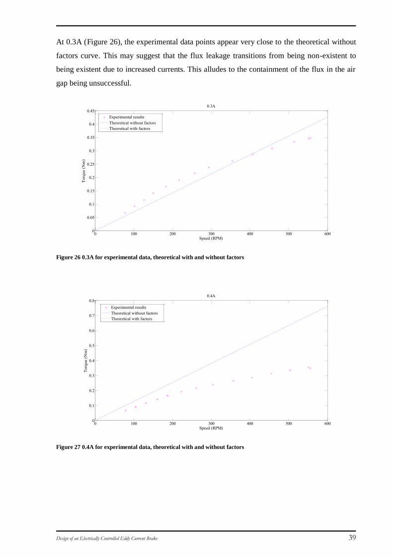
At 0.3A (Figure 26), the experimental data points appear very close to the theoretical without

factors curve. This may suggest that the flux leakage transitions from being non-existent to

being existent due to increased currents. This alludes to the containment of the flux in the air

gap being unsuccessful.

Figure 26 0.3A for experimental data, theoretical with and without factors

Figure 27 0.4A for experimental data, theoretical with and without factors

0 100 200 300 400 500 6000

0.05

0.1

0.15

0.2

0.25

0.3

0.35

0.4

0.450.3A

Speed (RPM)

To

rqu

e (N

m)

Experimental results

Theoretical without factors

Theoretical with factors

0 100 200 300 400 500 6000

0.1

0.2

0.3

0.4

0.5

0.6

0.7

0.80.4A

Speed (RPM)

To

rqu

e (N

m)

Experimental results

Theoretical without factors

Theoretical with factors

Design of an Electrically Controlled Eddy Current Brake 40

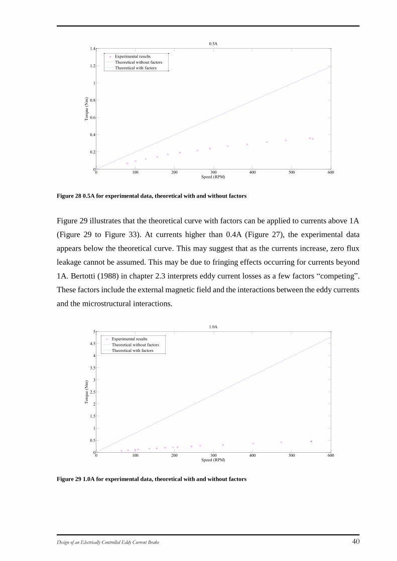
Figure 28 0.5A for experimental data, theoretical with and without factors

Figure 29 illustrates that the theoretical curve with factors can be applied to currents above 1A

(Figure 29 to Figure 33). At currents higher than 0.4A (Figure 27), the experimental data

appears below the theoretical curve. This may suggest that as the currents increase, zero flux

leakage cannot be assumed. This may be due to fringing effects occurring for currents beyond

1A. Bertotti (1988) in chapter 2.3 interprets eddy current losses as a few factors “competing”.

These factors include the external magnetic field and the interactions between the eddy currents

and the microstructural interactions.

Figure 29 1.0A for experimental data, theoretical with and without factors

0 100 200 300 400 500 6000

0.2

0.4

0.6

0.8

1

1.2

1.40.5A

Speed (RPM)

To

rqu

e (N

m)

Experimental results

Theoretical without factors

Theoretical with factors

0 100 200 300 400 500 6000

0.5

1

1.5

2

2.5

3

3.5

4

4.5

51.0A

Speed (RPM)

To

rqu

e (N

m)

Experimental results

Theoretical without factors

Theoretical with factors

Design of an Electrically Controlled Eddy Current Brake 41

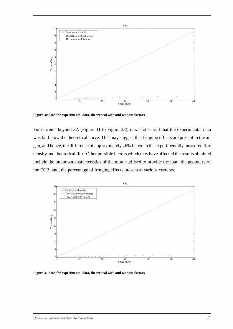
Figure 30 2.0A for experimental data, theoretical with and without factors

For currents beyond 3A (Figure 31 to Figure 33), it was observed that the experimental data

was far below the theoretical curve. This may suggest that fringing effects are present in the air

gap, and hence, the difference of approximately 46% between the experimentally measured flux

density and theoretical flux. Other possible factors which may have affected the results obtained

include the unknown characteristics of the motor utilised to provide the load, the geometry of

the ECB, and, the percentage of fringing effects present at various currents.

Figure 31 3.0A for experimental data, theoretical with and without factors

0 100 200 300 400 500 6000

2

4

6

8

10

12

14

16

18

202.0A

Speed (RPM)

To

rqu

e (N

m)

Experimental results

Theoretical without factors

Theoretical with factors

0 100 200 300 400 500 6000

5

10

15

20

25

30

35

40

453.0A

Speed (RPM)

To

rqu

e (N

m)

Experimental results

Theoretical without factors

Theoretical with factors

Design of an Electrically Controlled Eddy Current Brake 42

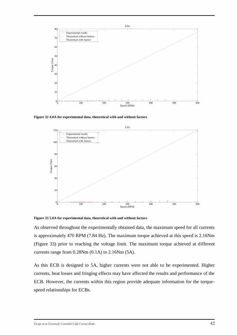
Figure 32 4.0A for experimental data, theoretical with and without factors

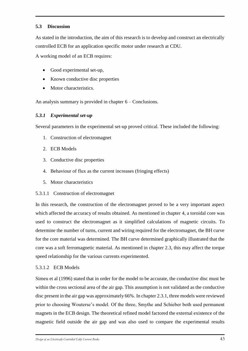
Figure 33 5.0A for experimental data, theoretical with and without factors

As observed throughout the experimentally obtained data, the maximum speed for all currents

is approximately 470 RPM (7.84 Hz). The maximum torque achieved at this speed is 2.16Nm

(Figure 33) prior to reaching the voltage limit. The maximum torque achieved at different

currents range from 0.28Nm (0.1A) to 2.16Nm (5A).

As this ECB is designed to 5A, higher currents were not able to be experimented. Higher

currents, heat losses and fringing effects may have affected the results and performance of the

ECB. However, the currents within this region provide adequate information for the torque-

speed relationships for ECBs.

0 100 200 300 400 500 6000

10

20

30

40

50

60

70

804.0A

Speed (RPM)

To

rqu

e (N

m)

Experimental results

Theoretical without factors

Theoretical with factors

0 100 200 300 400 500 6000

20

40

60

80

100

1205.0A

Speed (RPM)

To

rqu

e (N

m)

Experimental results

Theoretical without factors

Theoretical with factors

Design of an Electrically Controlled Eddy Current Brake 43

5.3 Discussion

As stated in the introduction, the aim of this research is to develop and construct an electrically

controlled ECB for an application specific motor under research at CDU.

A working model of an ECB requires:

Good experimental set-up,

Known conductive disc properties

Motor characteristics.

An analysis summary is provided in chapter 6 – Conclusions.

5.3.1 Experimental set-up

Several parameters in the experimental set-up proved critical. These included the following:

1. Construction of electromagnet

2. ECB Models

3. Conductive disc properties

4. Behaviour of flux as the current increases (fringing effects)

5. Motor characteristics

5.3.1.1 Construction of electromagnet

In this research, the construction of the electromagnet proved to be a very important aspect

which affected the accuracy of results obtained. As mentioned in chapter 4, a toroidal core was

used to construct the electromagnet as it simplified calculations of magnetic circuits. To

determine the number of turns, current and wiring required for the electromagnet, the BH curve

for the core material was determined. The BH curve determined graphically illustrated that the

core was a soft ferromagnetic material. As mentioned in chapter 2.3, this may affect the torque

speed relationship for the various currents experimented.

5.3.1.2 ECB Models

Simeu et al (1996) stated that in order for the model to be accurate, the conductive disc must be

within the cross sectional area of the air gap. This assumption is not validated as the conductive

disc present in the air gap was approximately 66%. In chapter 2.3.1, three models were reviewed

prior to choosing Wouterse’s model. Of the three, Smythe and Schieber both used permanent

magnets in the ECB design. The theoretical refined model factored the external existence of the

magnetic field outside the air gap and was also used to compare the experimental results

Design of an Electrically Controlled Eddy Current Brake 44

obtained. Ensuring the parameters are correct and similar to the primary conditions, the ECB

models and the experimental data should have similarities.

The aim of this thesis was to design an ECB for the test motor currently under research. The

conductive disc however, did not fully occupy the cross sectional area of the air gap. In an ideal

scenario, if the disc had a radius of 150mm, the experimental data may have provided

comparable to the theoretical curves. However, due to unknown factors being present during

experimenting, the relationship between the experimental results and the theoretical curves

cannot be validated.

5.3.1.3 Conductive disc properties

A factor in the ECB models that remains constant in the torque equation is the conductivity of

the conductive disc. This was an unknown parameter. Aluminium 6061 was assumption that

was made for this calculation. As observed in Equation 17, as the conductivity increases, the

torque increases.

Other factors that affect the torque speed curve include the thickness of the disc, the radius of

the conductive disc and the radius at which the pole is from the centre of the conductive disc.

5.3.1.4 Behaviour of Flux

The importance of the flux behaviour is crucial in this system. From the Table 2, it can be

observed that as the current increases, the percentage difference is approximately 4% for

currents up to 3A. The remainder of currents (4A and 5A) provide inconclusive results where

the percentage difference ranges from 23% to 46% respectively. As illustrated in Figure 24 to

Figure 33, due to factors such as the unknown behaviour of flux, fringing effects may be present

at higher currents. The percentage occurring is unknown.

The majority of the flux densities measured experimentally were relatively close. As mentioned

in chapter 2.1.2, Alfons et al (2009) and Sen (1997) demonstrated the effects of the air gap on

the BH curve. This has been validated for currents up to 3A. The remainder of the currents have

unknown factors acting within the ECB. Fringing effects may have been present, however the

percentage present at a given time is unknown.

As mentioned in 2.4, in order to predict the behaviour of the flux in an electromagnet, a FEA

analysis would need to be conducted. A 2D analysis in comparison to a 3D analysis would

provide lower computation time but would consequently not model certain external factors that

would be present in a 3D analysis.

Design of an Electrically Controlled Eddy Current Brake 45

5.3.1.5 Motor Characteristics

The motor utilised to provide the load for the ECB was set up in such a way that the user could

set a torque and the motor would adjust the speed accordingly.

In obtaining the torque readings, the torque sensor was always reset prior to conducting readings

for the currents (0.1A – 5A). However, the torque readings at 0A at the torque set point of

0.3Nm was not consistent throughout the readings for the different currents. The offset was

factored in the results by subtracting the offset from the quadratic function used to fit the

experimental torques.

5.4 Improvements

Electrically controlled ECBs can be constructed and improved in many ways. Improvements to

the final design presented in chapter 4 are as follows:

Use shorter strips when encasing it in fibreglass to avoid air gaps in the encasement of

electromagnet.

Air gap be cut precisely to 6-7 mm provided a 5mm disc used and must be square. If a

3mm disc is used, a 5mm air gap would be required.

Tape down the connections for the wires that were joined prior to encasement procedure.

Larger disc (150-200mm radius)

Utilising a larger disc can validate the assumption that the conductive disc to be within the cross

sectional area of the air gap. This may possibly validate the torque-speed relationship in

Wouterse’s model. However, a proposed new design is presented in the remainder of this

chapter.

The proposed new design with the following factors should be considered:

o Coils should be able to be spooled to avoid manual winding, this can also be

used in conjunction a measuring tool to confirm the length of copper wire used.

This will also aid in confirming the amount of turns in each branch or section.

o Design must be able to be integrated with existing equipment (motor, aluminium

disc).

o 150mm - 200mm radius aluminium disc.

o Adjustable air gap which allows for varying loads and speeds (use bearings and

door rollers).

Design of an Electrically Controlled Eddy Current Brake 46

o Utilise a hybrid ECB (permanent magnet and electromagnet) instead of a single

electromagnet.

The proposed design is illustrated in Appendix C: Proposed Design. This design utilises four

500 turn coils, 10 mm thick backing plate to complete the flux path, 3 mm thick aluminium

disc, and the current PMSM motor.

This design provides many advantages as well as disadvantages. The advantages include being

able to vary the speed by adjusting the air gap distance and spending minimal time winding the

coil as well as having a length to confirm the number of turns. Disadvantages consist of time to

specifically manufacture the objects, no spares and complex calculations.

5.5 Summary of results

This chapter presented known methods of determining the parameters of ECBs. However it did

not validate the assumptions as a whole due to the following factors:

1. The motor characteristics were unknown and therefore, provided offsets which were

estimated by fitting a quadratic curve and subtracting its offset from the torque values

obtained. The offset was not constant for the range of data collected.

2. The method in obtaining the majority of theoretical flux densities B was validated for

currents below 4A. The majority of the corresponding flux density values B was

significantly close to the values experimentally measured. However, at higher currents,

the percentage of difference increased.

Design of an Electrically Controlled Eddy Current Brake 47

6 Conclusion

Thus far, my thesis covering the design of an electrically controlled ECB, consisted of a

literature review of similar works of individuals, the determination of the magnetisation curve

of the core material, and the construction of the final design and construction.

In chapter 2, it was determined that Wouterse’s model would be utilised for comparison

purposes. It was also chosen due to its simplicity and application for electromagnets. As

mentioned in chapter 2.3.1, Schieber and Smythe’s models were complex and applied to

permanent magnets mainly.

The determination of the magnetisation curve provided the characteristics of the core material

and allowed for a realistic representation in terms of calculations for the theoretical torque,

speed and current. Upon completion of the construction of the final design, experimental results

were obtained to confirm the theoretical analysis. The load line method was used to determine

the flux density traveling through the air gap for specific currents. This was also compared to

experimentally measured flux densities taken on the motor test rig. The final design consisted

of using a toroidal core with two 1000 turn coils in parallel. Improvements were also determined

for the current electromagnet in chapter 5.4. The improvements also included a proposal of a

new experimental set-up and electromagnet.

Due to the geometry of the ECB developed in this research, the torque-speed relationship could

not be validated. Other unknown factors were also present in the experiments that could have

resulted in the torque speed relationship not being validated. These unknown factors may

possibly comprise of fringing effects, interactions of eddy currents and the external magnetic

field, and, conductive disc properties such as conductivity. However, the ECB has satisfied the

constraints of being able to achieve at least 0.3Nm and up to speeds of 9Hz.

Hence, from the analysis of the literature review, models and conceptual design, the ECB was

constructed and further developed. The working model was then used to verify the ECB with

Wouterse’s model and critical speed determination. Furthermore, the theoretical relationship

between torque and current could not be validated with the experimental results obtained due

to the factors discussed previously.

Design of an Electrically Controlled Eddy Current Brake 48

7 Future Works

Future works include but are not limited to:

Characterisation the motor.

3D FEA analysis of the ECB for behaviour of flux.

Determination of the behaviour of flux when the rotating aluminium disc does not fully

occupy the length of the air gap.

New mounting system with proposed electromagnet design

Investigate varying the loads and speeds by adjusting the amount of disc present in the

air gap.

Application of alternating current for varying torque loads.

Hybrid braking system (both permanent magnets and electromagnets)

The above future works allows for the comparison between permanent magnets versus

electromagnets as well as the behaviour of flux which has proved to be a critical factor in the

results obtained.

Maintaining the order of future works would find that:

Characterising the motor would minimise any losses, may potentially determine any losses and

take into account the torque offset which was observed throughout this thesis.

Conducting a FEA on the electromagnet would determine the behaviour of flux for increasing

currents. FEA can also be used to predict the behaviour of the torque-speed curve to compare

with experimental data. This method can also be used to determine the behaviour of flux when

the conductive disc is not within the air gap.

The new mounting system for the proposed electromagnet provides the opportunity to redesign

and minimise losses in the mounting system. This may minimise any torque offsets in future

experiments.

The investigation of varying the loads and speeds by adjusting the amount of disc present in the

air gap will allow minimisation of unknown factors and can potentially be more accurate than

the permanent magnet ECB used in current experiments.

Design of an Electrically Controlled Eddy Current Brake 49

Finally, applying AC currents through the ECB which will see different behaviour than when

DC currents were applied. This will allow for varying torque loads to be researched once the

above works have been completed.

Design of an Electrically Controlled Eddy Current Brake 50

8 References

[1] E. G. Thomas and A. J. Meadows, Maxwell's Equations and their Applications. Bristol,

England: Adam Hilger Ltd, 1985.

[2] W. R. Smythe, "On eddy currents in a rotating disk," Electrical Engineering, vol. 61,

pp. 681-684, 1942.

[3] B. S. Guru and H. R. Hiziroglu, Electromagnetic Field Theory Fundamentals. Boston,

Massachusetts: PWS Publishing Company, 1998.

[4] J. Bird, Electrical and Electronic Prinicples and Technology, Third ed. Massachusetts,

USA: Elsevier Ltd, 2007.

[5] P. C. Sen, Principles of Electric Machines and Power Electronics, Second ed. Canada:

John Wiley & Sons Inc., 1997.

[6] K. Karakoc, "Modelling and Design Optimization of Electromechanical Brake Actuator

Using Eddy Currents," Mechanical Engineering PhD, Department of Mechanical

Engineering, University of Victoria, 2012.

[7] G. Schweitzer and E. H. Maslen, Magnetic Bearings: Theory, Design, and Application

to Rotating Machinery: Springer, 2009.

[8] G. Bertotti, "General properties of power losses in soft ferromagnetic materials,"

Magnetics, IEEE Transactions on, vol. 24, pp. 621-630, 1988.

[9] G. Heins, "Control Methods for Smooth Operation of Permanent Magnet Synchronous

AC Motors," Doctor of Philosophy, Charles Darwin University, 2008.

[10] L. Barnes, J. Hardin, C. A. Gross, and D. Wasson, "An eddy current braking system,"

in System Theory, 1993. Proceedings SSST '93., Twenty-Fifth Southeastern Symposium

on, 1993, pp. 58-62.

[11] J. Seok-Myeong and L. Sung-Ho, "Comparison of three types of permanent magnet

linear eddy-current brakes according to magnetization pattern," Magnetics, IEEE

Transactions on, vol. 39, pp. 3004-3006, 2003.

[12] D. M. Ma and J. Shiau, "The Design of Eddy-Current Magnet Brakes," Transactions of

the Canadian Society for Mechanical Engineering, vol. 35, p. 37, 2011.

[13] X. Zhao and C. Ji, "Analysis of flux leakage in novel permanent magnet type eddy

current retarder for vehicle applications," in Vehicle Power and Propulsion Conference,

2008. VPPC '08. IEEE, 2008, pp. 1-4.

[14] V. C. A. Ferraro, Electromagnetic Theory. London: The Athlone Press, University of

London, 1956.

[15] K. Lee and K. Park, "Optimal robust control of a contactless brake system using an eddy

current," Mechatronics, vol. 9, pp. 615-631, 9// 1999.

[16] A. H. C. Gosline and V. Hayward, "Eddy Current Brakes for Haptic Interfaces: Design,

Identification, and Control," Mechatronics, IEEE/ASME Transactions on, vol. 13, pp.

669-677, 2008.

[17] H. D. Wiederick, N. Gauthier, D. A. Campbell, and P. Rochon, "Magnetic Braking:

Simple theory and experiment," American Journal of Physics, vol. Volume 55, pp. 500-

503, 1987.

Design of an Electrically Controlled Eddy Current Brake 51

[18] A. H. Gosline, G. Campion, and V. Hayward, On the use of eddy current brakes as

tunable, fast turn-on viscous dampers for haptic rendering, 2006.

[19] N. J. Caldwell and J. R. M. Taylor, "Eddy-Current Actuator for a Variable Pitch Air

Turbine," in Proc. Third European Wave Power Conference, Patras, Greece, 1998.

[20] E. Simeu and D. Georges, "Modeling and control of an eddy current brake," Control

Engineering Practice, vol. 4, pp. 19-26, 1// 1996.

[21] J. H. Wouterse, "Critical torque and speed of eddy current brake with widely separated

soft iron poles," Electric Power Applications, IEE Proceedings B, vol. 138, pp. 153-

158, 1991.

[22] D. Schieber, "Braking torque on rotating sheet in stationary magnetic field," Electrical

Engineers, Proceedings of the Institution of, vol. 121, pp. 117-122, 1974.

[23] M. Heald, "Magnetic Braking: Improved Theory," American Journal of Physics, vol.

56, 1988.

[24] M. O. Gulbahce, D. A. Kocabas, and A. K. Atalay, "A study to determine the act of

excitation current on braking torque for a low power eddy current brake," in Electric

Machines & Drives Conference (IEMDC), 2013 IEEE International, 2013, pp. 1321-

1325.

[25] M. O. Gulbahce, D. A. Kocabas, and I. Habir, "Finite elements analysis of a small power

eddy current brake," in MECHATRONIKA, 2012 15th International Symposium, 2012,

pp. 1-5.

[26] S. E. Gay and M. Ehsani, "Parametric analysis of eddy-current brake performance by 3-

D finite-element analysis," Magnetics, IEEE Transactions on, vol. 42, pp. 319-328,

2006.

[27] M. Hecquet, P. Brochet, J. Lee Sang, and P. Delsalle, "A linear eddy current braking

system defined by finite element method," Magnetics, IEEE Transactions on, vol. 35,

pp. 1841-1844, 1999.

[28] W. J. Duffin, Electricity and magnetism. London ; New York: McGraw-Hill, 1990.

[29] W. L. Soong, "BH Curve and Iron Loss Measurements for Magnetic Materials," Power

Engineering Briefing Notes (PEBN), p. 4, 2008.

[30] N. E. R. Center. (2012, 04-10-2013). Material Properties Tables Electrical

Conductivity and Resistivity. Available: http://www.ndt-ed.org/index_flash.htm

[31] M. Z. Bahorom, M. Z. Nuawi, G. Priyandoko, and S. M. Harris, "Eddy Current Braking

Experiment using Brake Disc from aluminium series of Al6061 and Al7075," in 1st

International Conference on Mechanical Engineering Research 2011, 2012.

[32] Keywolf. American Wire Gauge (AWG) Sizes and Current Limits. Available:

http://www.keywolf.com/American_Wire_Gauge.php

[33] PolySource. (2014, 19/04/2014). Polyurethane Products. Available:

http://www.polysource.com.au/products/polyurethane.html

[34] Molded Fiber Glass Companies. (2014, 19/04/2014). Polyurethane Resins. Available:

http://www.moldedfiberglass.com/materials/polyurethane-resins

[35] Molded Fibre Glass Companies. (2014, 19/04/2014). Epoxy Resins. Available:

http://www.moldedfiberglass.com/materials/epoxy-resins

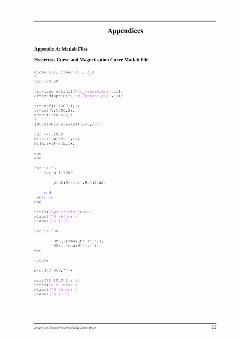
Design of an Electrically Controlled Eddy Current Brake 52

Appendices

Appendix A: Matlab Files

Hysteresis Curve and Magnetisation Curve Matlab File

close all, clear all, clc % for i=0:30

vsf=load(sprintf('%d_vsense.txt',i)); cf=load(sprintf('%d_current.txt',i));

tt=(vsf(1:1000,1)); vv=vsf(1:1000,2); cc=cf(1:1000,2); % [Bt,H]=hysteresis(tt,vv,cc);

for m=1:1000 Bt1(i+1,m)=Bt(1,m); H1(m,i+1)=H(m,1);

end end

for i=1:31 for m=1:1000

plot(H1(m,i),Bt1(i,m))

end hold on end

title('Hysteresis Curve') xlabel('H (At/m)') ylabel('B (T)')

for i=1:30

Bt2(i)=max(Bt1(i,:)); H2(i)=max(H1(:,i)); end

figure

plot(H2,Bt2,'*')

axis([0,1050,1,2.3]) title('B-H Curve') xlabel('H (At/m)') ylabel('B (T)')

Design of an Electrically Controlled Eddy Current Brake 53

Hysteresis Function File

function [ Bt,H ] = hysteresis(tt,vv,cc ) %UNTITLED2 Summary of this function goes here % Detailed explanation goes here\

Nmain=50; lcore=pi*0.1525;

%mean of vsense and current mvsense=mean(vv); mcurrent=mean(cc);

vv1=vv(1:1000)-mvsense; cc1=cc-mcurrent; %remove dc offset

%The magnetic Field Intensity (H) eqn 1 H=(Nmain.*cc)/lcore;

Nsense=15; Acore=1360*(10^-6); delt=0.02*(10^(-3)); % for k=1:1000

% lambdas(k,1)=trapz(vsense(k)); % lambdas(k,1)=vsense(k); lambdas1(1)=vv1(1)*delt;

lambdas1(k+1)=lambdas1(k)+(vv1(k)*delt);

end

mlambdas=mean(lambdas1); lambdas2=lambdas1-mlambdas; %remove dc offset

%Flux Density (B) eqn 3 B=lambdas2/(Acore*Nsense);

Bt=B(1,2:1001);

end

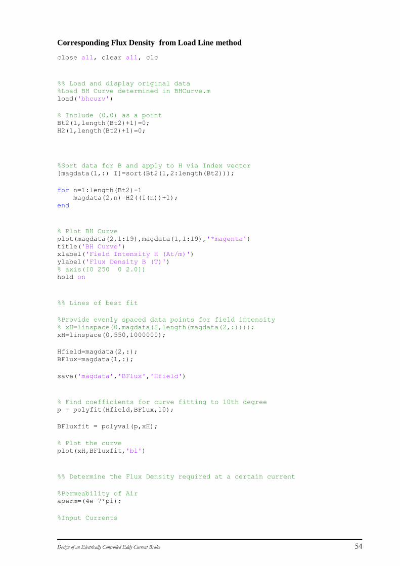
Design of an Electrically Controlled Eddy Current Brake 54

Corresponding Flux Density from Load Line method

close all, clear all, clc

%% Load and display original data %Load BH Curve determined in BHCurve.m load('bhcurv')

% Include (0,0) as a point Bt2(1,length(Bt2)+1)=0; H2(1,length(Bt2)+1)=0;

%Sort data for B and apply to H via Index vector [magdata(1,:) I]=sort(Bt2(1,2:length(Bt2)));

for n=1:length(Bt2)-1 magdata(2,n)=H2((I(n))+1); end

% Plot BH Curve plot(magdata(2,1:19),magdata(1,1:19),'*magenta') title('BH Curve') xlabel('Field Intensity H (At/m)') ylabel('Flux Density B (T)') % axis([0 250 0 2.0]) hold on

%% Lines of best fit

%Provide evenly spaced data points for field intensity % xH=linspace(0,magdata(2,length(magdata(2,:)))); xH=linspace(0,550,1000000);

Hfield=magdata(2,:); BFlux=magdata(1,:);

save('magdata','BFlux','Hfield')

% Find coefficients for curve fitting to 10th degree p = polyfit(Hfield,BFlux,10);

BFluxfit = polyval(p,xH);

% Plot the curve plot(xH,BFluxfit,'bl')

%% Determine the Flux Density required at a certain current

%Permeability of Air aperm=(4e-7*pi);

%Input Currents

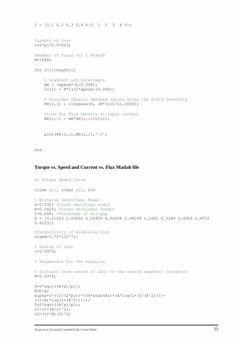
Design of an Electrically Controlled Eddy Current Brake 55

I = [0.1 0.2 0.3 0.4 0.5 1 2 3 4 5];

%Length of Core L=2*pi*0.07625;

%Number of Turns for 1 Branch N=1048;

for i=1:length(I)

% Gradient and intercepts mm = -aperm*(L/0.008); cc(i) = N*I(i)*aperm/(0.008);

% Provides equally speaced values along the Field Intensity HH(i,:) = linspace(0, (N*I(i)/L),1000);

%Line for Flux Density at input current BB(i,:) = mm*HH(i,:)+cc(i);

plot(HH(i,:),BB(i,:),'-k')

end

Torque vs. Speed and Current vs. Flux Matlab file

%% Torque Speed Curve

close all, clear all, clc

% Wouterse (modified) Model a=0.032; %Cross sectional width b=0.0425; %Cross sectional length t=0.008; %Thickness of air-gap B = [0.01623 0.03266 0.04909 0.06558 0.08198 0.1641 0.3286 0.4929 0.6572

0.8223];

%Conductivity of Aluminium Disc sigma=2.72*(10^7);

% Radius of Disc r=0.0975;

% Parameters for the equation

% Distance from centre of disc to the centre magnetic footprint R=0.0975;

D=2*sqrt((b*a)/pi); A=b/a; alpha=1-((1/(2*pi))*((4*atan(A))+(A*log(1+(1/(A^2))))-

((1/A)*log(1+(A^2))))); D=2*sqrt((b*a)/pi); c1=(1+(R/r)^2); c2=((r-R)/D)^2;

Design of an Electrically Controlled Eddy Current Brake 56

c3=1/(c1*c2); c4=abs(0.5*(1-((0.25)*c3))); % Frequencies to test f=0:0.0005:10; v=2*pi*r*f; w=2*pi*f; % Conversion RPM rpm=w*(60/(2*pi));

% Torque Speed Curve Formula for nn=1:length(B) for g=1:20001

T(nn,g)=(a*b*t*sigma*(B(nn)^2)*v(1,g)*r)*0.6689; TF(nn,g)=(a*b*t*sigma*alpha*c4*(B(nn)^2)*v(1,g)*r)*0.6689;

end end

figure plot(rpm,T) Title('Torque vs. Speed (via Experimental values of BH Curve)') xlabel('Speed (RPM)') ylabel('Torque (Nm)') legend('0.1A','0.2A','0.3A','0.4A','0.5A','1.0A','2.0A','3.0A','4.0A','5.0A

'); hold on axis([0 600 0 3])

%% Load Experimental Data

for i=1:5 Exp=load(sprintf('0_%d.txt',i));

for n=1:length(Exp(:,1)) Texp(n,i)=Exp(n,1); W(n,i)=Exp(n,2); end

Exp=load(sprintf('%d.txt',i));

for n=1:length(Exp(:,1)) Texp(n,i+5)=Exp(n,1); W(n,i+5)=Exp(n,2); end end

%% plot them all individually figure T01=Texp(1:13,1)-0.079; S01=W(1:13,1)*60; plot(S01,T01,'*magenta',rpm,T(1,:),rpm,TF(1,:)); title('0.1A') xlabel('Speed (RPM)') ylabel('Torque (Nm)') legend('Experimental results','Theoretical without factors','Theoretical

with factors')

% figure

Design of an Electrically Controlled Eddy Current Brake 57

T02=Texp(1:13,2)-0.23; S02=W(1:13,2)*60; plot(S02,T02,'*magenta',rpm,T(2,:),rpm,TF(2,:)); title('0.2A') xlabel('Speed (RPM)') ylabel('Torque') legend('Experimental results','Theoretical without factors','Theoretical

with factors')

% figure T03=Texp(1:14,3)-0.3; S03=W(1:14,3)*60; plot(S03,T03,'*magenta',rpm,T(3,:),rpm,TF(3,:)); title('0.3A') xlabel('Speed (RPM)') ylabel('Torque (Nm)') legend('Experimental results','Theoretical without factors','Theoretical

with factors')

% figure T04=Texp(1:14,4)-0.29; S04=W(1:14,4)*60; plot(S04,T04,'*magenta',rpm,T(4,:),rpm,TF(4,:)); title('0.4A') xlabel('Speed (RPM)') ylabel('Torque (Nm)') legend('Experimental results','Theoretical without factors','Theoretical

with factors')

%

figure T05=Texp(1:14,5)-0.23; S05=W(1:14,5)*60; plot(S05,T05,'*magenta',rpm,T(5,:),rpm,TF(5,:)); title('0.5A') xlabel('Speed (RPM)') ylabel('Torque (Nm)') legend('Experimental results','Theoretical without factors','Theoretical

with factors')

% % figure T1=Texp(1:16,6)-0.21; S1=W(1:16,6)*60; plot(S1,T1,'*magenta',rpm,T(6,:),rpm,TF(6,:)); title('1.0A') xlabel('Speed (RPM)') ylabel('Torque (Nm)') legend('Experimental results','Theoretical without factors','Theoretical

with factors')

% figure T2=Texp(1:20,7)-0.22; S2=W(1:20,7)*60; plot(S2,T2,'*magenta',rpm,T(7,:),rpm,TF(7,:)); title('2.0A')

Design of an Electrically Controlled Eddy Current Brake 58

xlabel('Speed (RPM)') ylabel('Torque (Nm)') legend('Experimental results','Theoretical without factors','Theoretical

with factors')

figure T3=Texp(1:27,8)-0.22; S3=W(1:27,8)*60; plot(S3,T3,'*magenta',rpm,T(8,:),rpm,TF(8,:)); title('3.0A') xlabel('Speed (RPM)') ylabel('Torque (Nm)') legend('Experimental results','Theoretical without factors','Theoretical

with factors')

figure T4=Texp(1:26,9)-0.19; S4=W(1:26,9)*60; plot(S4,T4,'*magenta',rpm,T(9,:),rpm,TF(9,:)); hold on title('4.0A') xlabel('Speed (RPM)') ylabel('Torque (Nm)') legend('Experimental results','Theoretical without factors','Theoretical

with factors')

figure T5=Texp(1:28,10)-0.28; S5=W(1:28,10)*60; plot(S5,T5,'*magenta',rpm,T(10,:),rpm,TF(10,:)); title('5.0A') xlabel('Speed (RPM)') ylabel('Torque (Nm)') legend('Experimental results','Theoretical without factors','Theoretical

with factors')

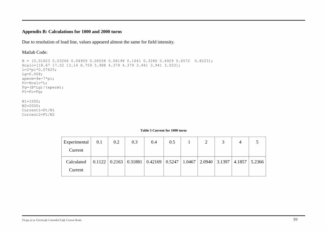
Design of an Electrically Controlled Eddy Current Brake 59

Appendix B: Calculations for 1000 and 2000 turns

Due to resolution of load line, values appeared almost the same for field intensity.

Matlab Code:

B = [0.01623 0.03266 0.04909 0.06558 0.08198 0.1641 0.3286 0.4929 0.6572 0.8223]; Hcalc=[18.67 17.52 13.14 8.759 5.988 4.379 4.379 3.941 3.941 3.503]; L=2*pi*0.07625; Lg=0.008; aperm=4e-7*pi; Fc=Hcalc*L; Fg=(B*Lg)/(aperm); Ft=Fc+Fg;

N1=1000; N2=2000; Current1=Ft/N1 Current2=Ft/N2

Table 5 Current for 1000 turns

Experimental

Current

0.1 0.2 0.3 0.4 0.5 1 2 3 4 5

Calculated

Current

0.1122 0.2163 0.31881 0.42169 0.5247 1.0467 2.0940 3.1397 4.1857 5.2366

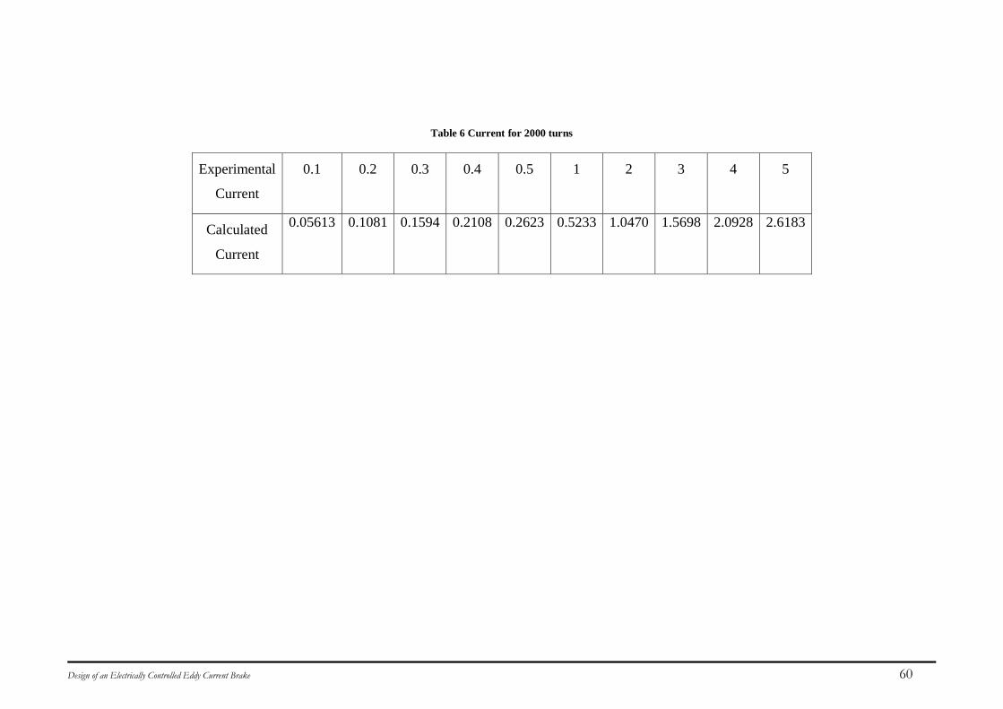
Design of an Electrically Controlled Eddy Current Brake 60

Table 6 Current for 2000 turns

Experimental

Current

0.1 0.2 0.3 0.4 0.5 1 2 3 4 5

Calculated

Current

0.05613 0.1081 0.1594 0.2108 0.2623 0.5233 1.0470 1.5698 2.0928 2.6183

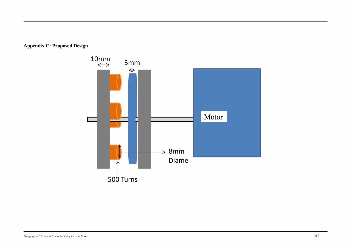
Design of an Electrically Controlled Eddy Current Brake 61

Appendix C: Proposed Design

3mm

500 Turns

10mm

8mm Diameter

Motor