Continuous Probability Distributions

Exponential, Erlang, Gamma

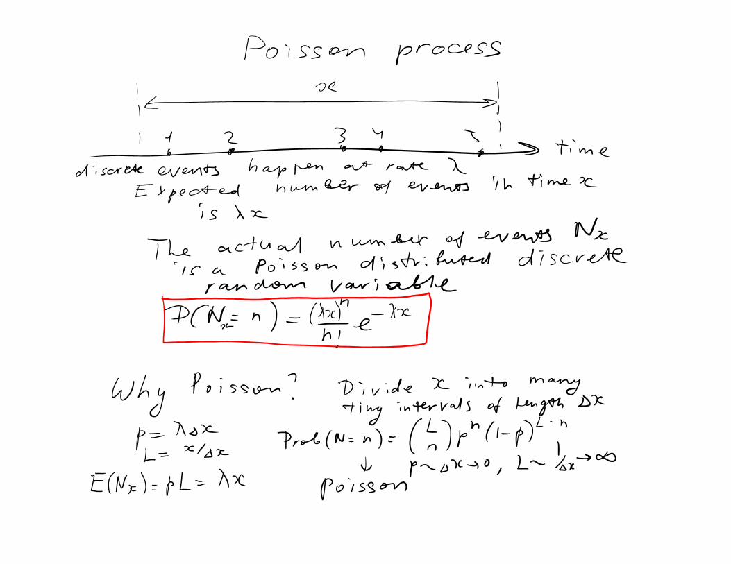
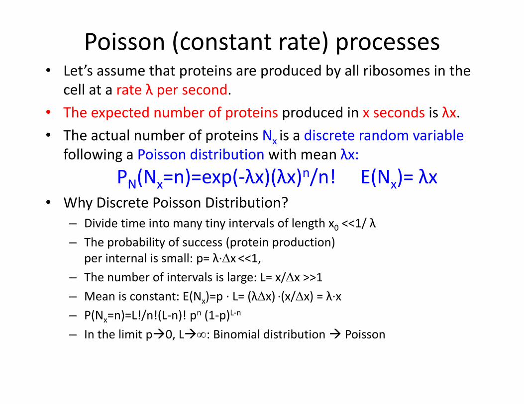
Poisson (constant rate) processes• Let’s assume that proteins are produced by all ribosomes in the 

cell at a rate λ per second. • The expected number of proteins produced in x seconds is λx.• The actual number of proteins Nx is a discrete random variable

following a Poisson distribution with mean λx:             PN(Nx=n)=exp(‐λx)(λx)n/n!     E(Nx)= λx

• Why Discrete Poisson Distribution?  – Divide time into many tiny intervals of length x0 <<1/ λ– The probability of success (protein production) 

per internal is small: p= λ∙x <<1,– The number of intervals is large: L= x/x >>1– Mean is constant: E(Nx)=p ∙ L= (λx) ∙(x/x) = λ∙x– P(Nx=n)=L!/n!(L‐n)! pn (1‐p)L‐n

– In the limit p0, L: Binomial distribution  Poisson

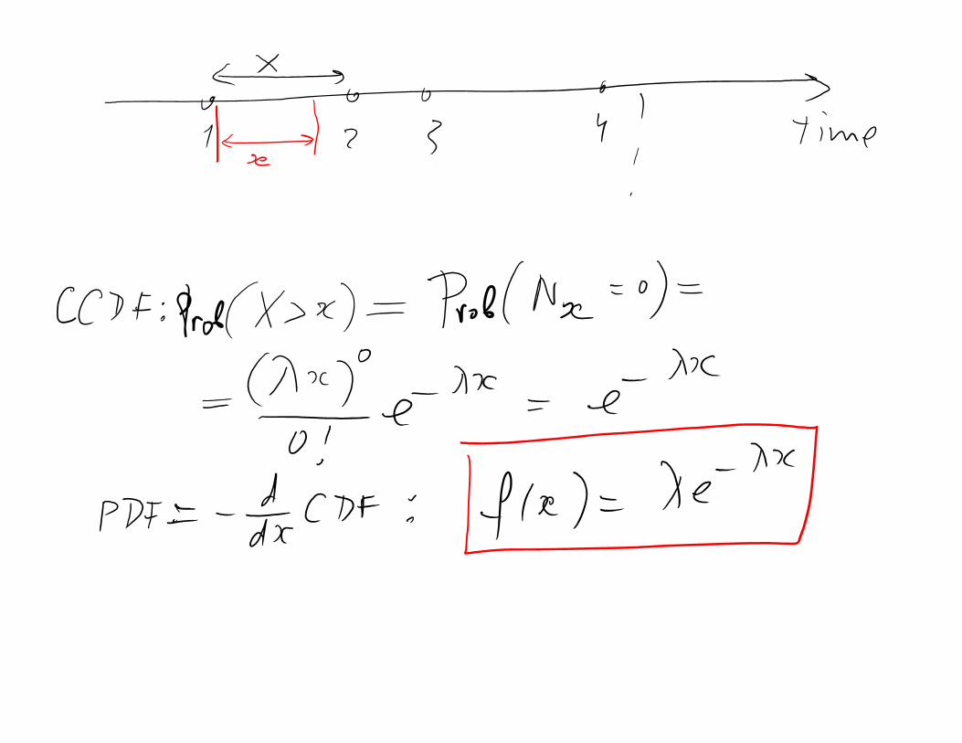
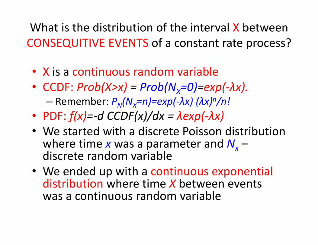
What is the distribution of the interval X between CONSEQUITIVE EVENTS of a constant rate process?

• X is a continuous random variable• CCDF: Prob(X>x) = Prob(NX=0)=exp(‐λx). 

– Remember: PN(NX=n)=exp(‐λx) (λx)n/n!• PDF: f(x)=‐d CCDF(x)/dx = λexp(‐λx)• We started with a discrete Poisson distribution where time x was a parameter and Nx –discrete random variable 

• We ended up with a continuous exponential distribution where time X between events was a continuous random variable 

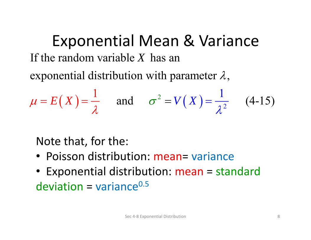
Exponential Mean & Variance

Sec 4‐8 Exponential Distribution 8

22

If the random variable has an exponential distribution with parameter ,

and (4-1511 )VE

X

X X

Note that, for the:• Poisson distribution: mean= variance• Exponential distribution: mean = standard deviation = variance0.5

9

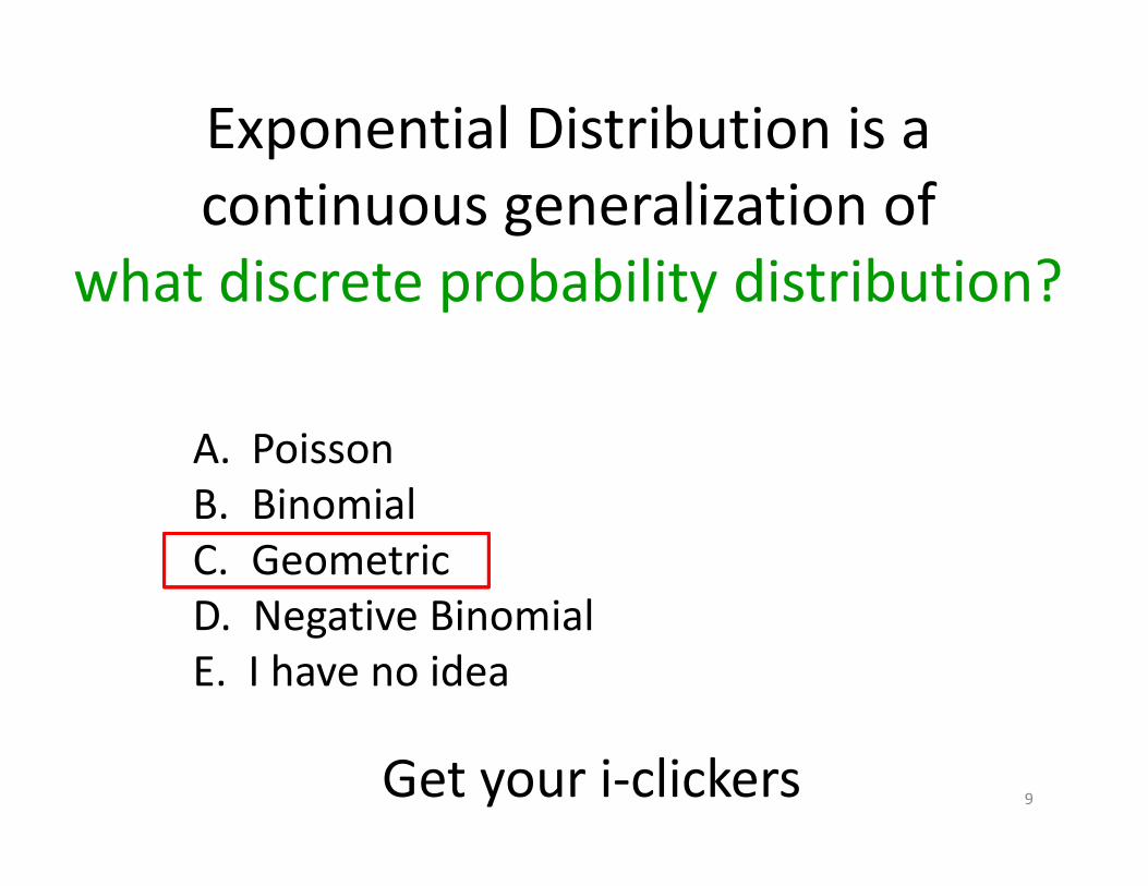
Exponential Distribution is a continuous generalization of 

what discrete probability distribution?

A. PoissonB. BinomialC. GeometricD.  Negative BinomialE.  I have no idea

Get your i‐clickers

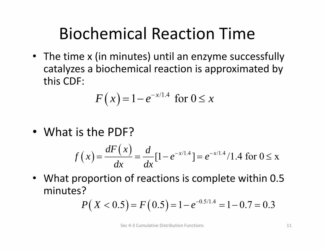
Biochemical Reaction Time• The time x (in minutes) until an enzyme successfully catalyzes a biochemical reaction is approximated by this CDF:

• What is the PDF?

• What proportion of reactions is complete within 0.5  minutes?

Sec 4‐3 Cumulative Distribution Functions 11

/1.4 /1.4[1 ] /1.4 for 0 xx xdF x df x e edx dx

0.5/1.40.5 0.5 1 1 0.7 0.3P X F e

/1.41 for 0xF x e x

12

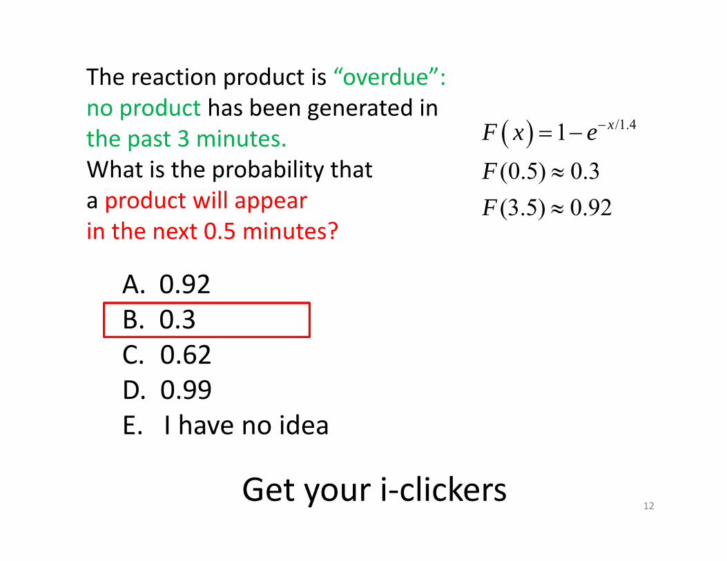
The reaction product is “overdue”: no product has been generated in the past 3 minutes. What is the probability that a product will appear in the next 0.5 minutes?

A. 0.92B. 0.3C. 0.62D.  0.99E.   I have no idea

Get your i‐clickers

/1.41 (0.5) 0.3(3.5) 0.92

xF x eFF

Exponential Distribution in Reliability

• The reliability of electronic components is often modeled by the exponential distribution.  A chip might have mean time to failure of 40,000 operating hours.

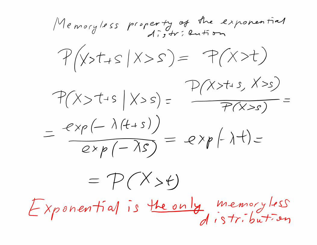
• The memoryless property implies that the component does not wear out – the probability of failure in the next hour is constant, regardless of the component age.

• The reliability of mechanical components do have a memory – the probability of failure in the next hour increases as the component ages.  

Sec 4‐8 Exponential Distribution 19

Erlang Distribution

• The Erlang distribution is a generalization of the exponential distribution.

• The exponential distribution models the time interval to the 1st event, while the 

• Erlang distribution models the timeinterval to the rth event, i.e., a sum of r exponentially distributed variables.

• The exponential, as well as Erlang distributions, is based on the constant rate  Poisson process.

20

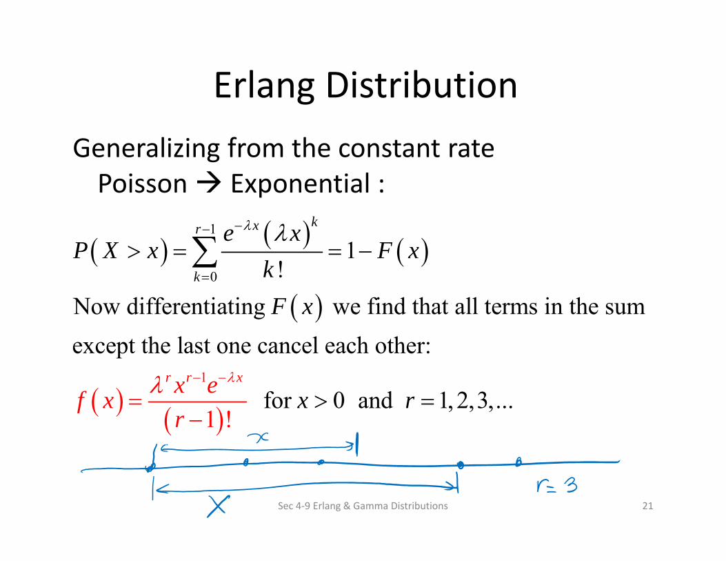
Erlang DistributionGeneralizing from the constant rate Poisson  Exponential :

Sec 4‐9 Erlang & Gamma Distributions 21

1

1

01

!Now differentiating we find that all terms in the sumexcept the last one cancel each other:

for 0 and 1,2,3,. .1

. !

r

kr

k

r x

x

x ef

e xP X x F x

k

rxr

F x

x

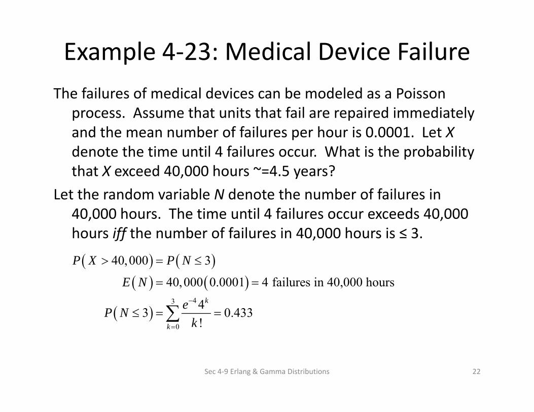
Example 4‐23: Medical Device FailureThe failures of medical devices can be modeled as a Poisson 

process.  Assume that units that fail are repaired immediately and the mean number of failures per hour is 0.0001.  Let Xdenote the time until 4 failures occur.  What is the probability that X exceed 40,000 hours ~=4.5 years?

Let the random variable N denote the number of failures in 40,000 hours.  The time until 4 failures occur exceeds 40,000 hours iff the number of failures in 40,000 hours is ≤ 3.

Sec 4‐9 Erlang & Gamma Distributions 22

43

0

40,000 3

40,000 0.0001 4 failures in 40,000 hours

43 0.433!

k

k

P X P N

E N

eP Nk

23

Erlang Distribution is a continuous generalization of 

what discrete probability distribution?

A. PoissonB. BinomialC. GeometricD.  Negative BinomialE.  I have no idea

Get your i‐clickers

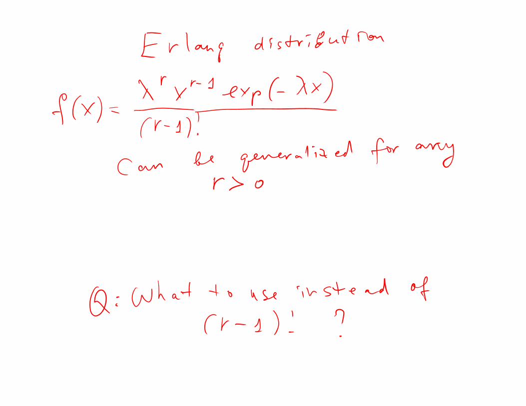
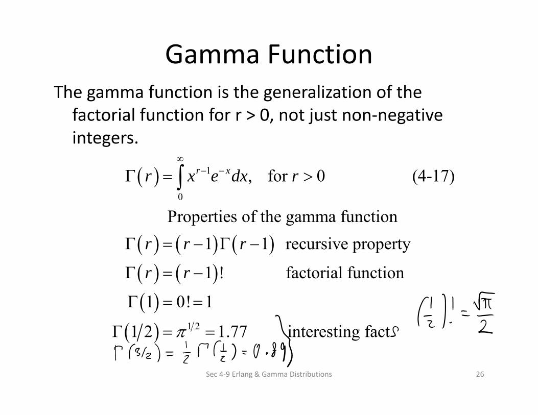
Gamma FunctionThe gamma function is the generalization of the factorial function for r > 0, not just non‐negative integers.

Sec 4‐9 Erlang & Gamma Distributions 26

1

0

1 2

, for 0 (4-17)

Properties of the gamma function1 1 recursive property

1 ! factorial function

1 0! 1

1 2 1.77 interesting fact

r xr x e dx r

r r r

r r

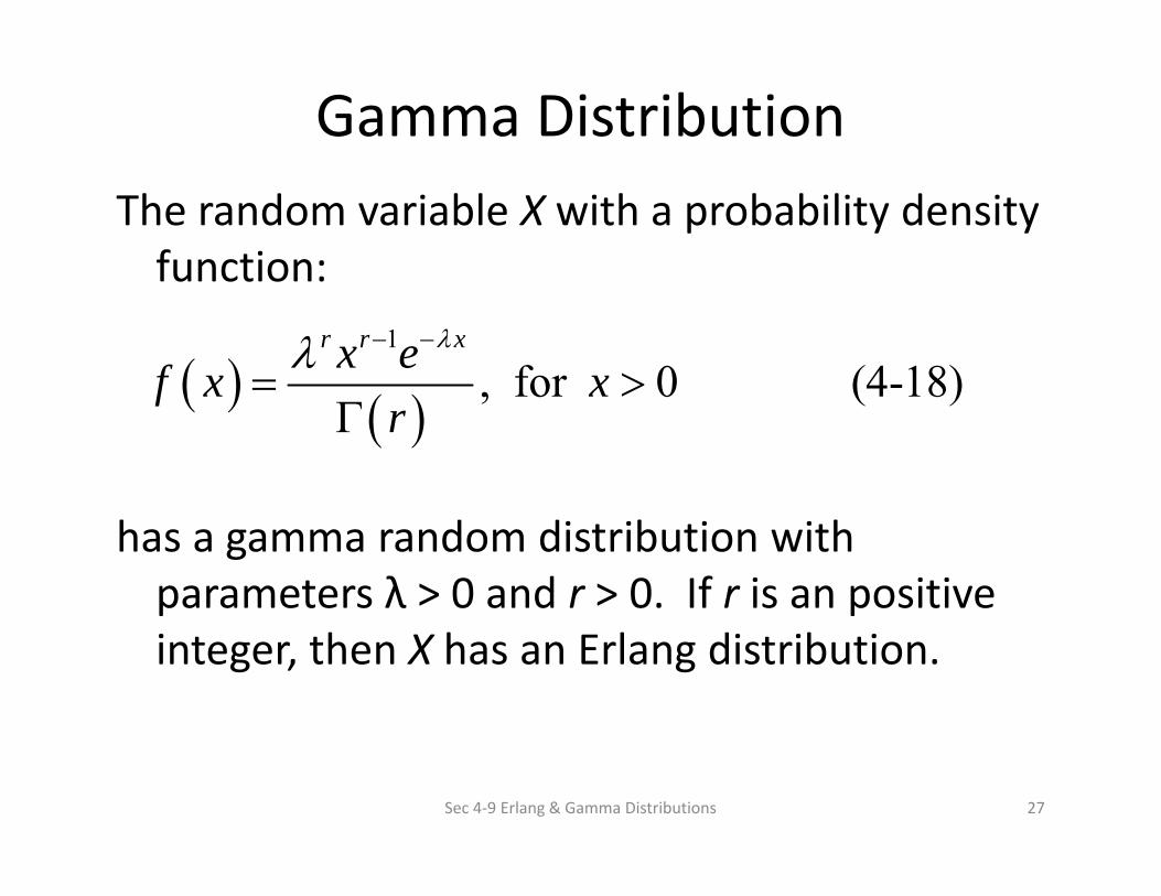
Gamma DistributionThe random variable X with a probability density function:

has a gamma random distribution with parameters λ > 0 and r > 0.  If r is an positive integer, then X has an Erlang distribution.

Sec 4‐9 Erlang & Gamma Distributions 27

1

, for 0 (4-18)r r xx ef x x

r

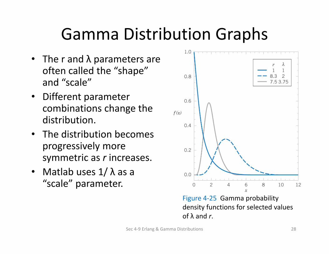
Gamma Distribution Graphs• The r and λ parameters are 

often called the “shape” and “scale”

• Different parameter combinations change the distribution.

• The distribution becomes progressively more symmetric as r increases.

• Matlab uses 1/ λ as a “scale” parameter.

Sec 4‐9 Erlang & Gamma Distributions 28

Figure 4‐25  Gamma probability density functions for selected values of λ and r.

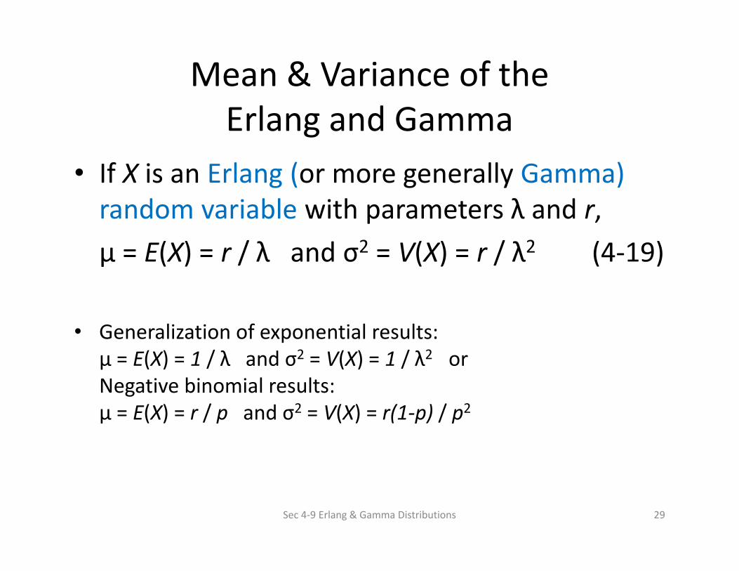
Mean & Variance of the Erlang and Gamma

• If X is an Erlang (or more generally Gamma)random variable with parameters λ and r,μ = E(X) = r / λ and σ2 = V(X) = r / λ2 (4‐19)

• Generalization of exponential results:μ = E(X) = 1 / λ and σ2 = V(X) = 1 / λ2 or Negative binomial results:μ = E(X) = r / p and σ2 = V(X) = r(1‐p) / p2

Sec 4‐9 Erlang & Gamma Distributions 29

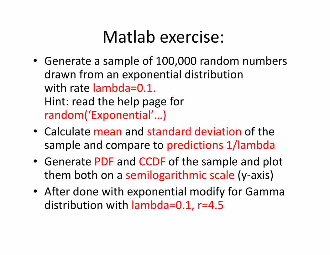
Matlab exercise: • Generate a sample of 100,000 random numbers drawn from an exponential distributionwith rate lambda=0.1. Hint: read the help page for random(‘Exponential’…)

• Calculate mean and standard deviation of the sample and compare to predictions 1/lambda

• Generate PDF and CCDF of the sample and plot them both on a semilogarithmic scale (y‐axis)

• After done with exponential modify for Gammadistribution with lambda=0.1, r=4.5

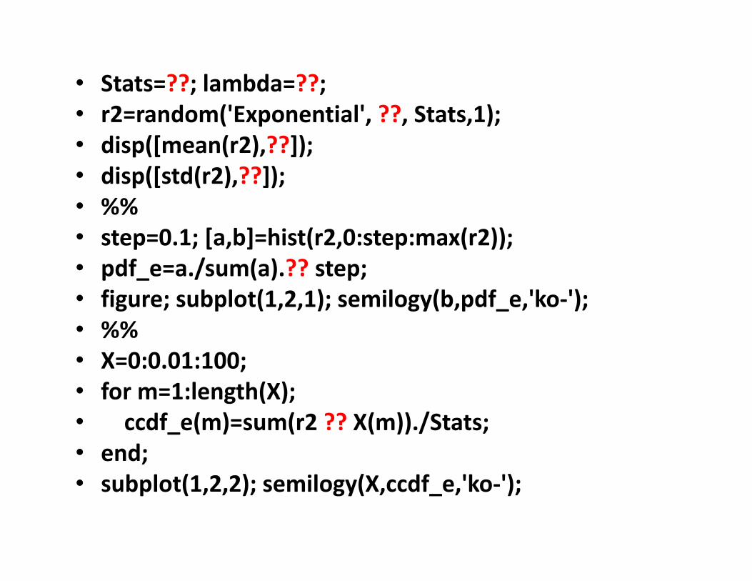
• Stats=??; lambda=??;• r2=random('Exponential', ??, Stats,1);• disp([mean(r2),??]);• disp([std(r2),??]);• %%• step=0.1; [a,b]=hist(r2,0:step:max(r2));• pdf_e=a./sum(a).?? step;• figure; subplot(1,2,1); semilogy(b,pdf_e,'ko‐');• %%• X=0:0.01:100; • for m=1:length(X); • ccdf_e(m)=sum(r2 ?? X(m))./Stats; • end;• subplot(1,2,2); semilogy(X,ccdf_e,'ko‐');

Credit: XKCD comics