COMPARISON OF NUMERICAL METHODS IN PREDICTING THE

GROWTH OF NORMAL AGRICULTURAL ASSETS

Godspower C. Abanum

Department of Mathematics/Statistics,

Ignatius Ajuru University of Education, Port Harcourt, Nigeria

Corresponding Author: godspower.abanum@iaue.edu.ng

Abstract

In this paper, I considered the comparison of numerical methods in predicting the biodiversity gain due to

the variation of α1 and α2 together on biodiversity scenario. However, when the model parameter values

α1 and α2 are increase, the normal agricultural variable also changes. By comparing the patterns of growth

in these two interacting normal agricultural data, we have finite instance of biodiversity due to the

application of four numerical methods such as ODE45, ODE23, ODE23tb and ODE15s. We have found

the numerical prediction upon using these four numerical methods which are similar and robust, hence we

have considered ODE45 numerical simulation to be computationally more efficient than the other three

methods. The novel result we have obtained in this study have not been seen elsewhere.

Keywords: ODE45, ODE23, ODE23tb, ODE15s, Normal Agriculture

1. INTRODUCTION

Modeling and simulation of dynamical systems has always been an important issue in Science,

Engineering, Biological sector, Medical sector and Agricultural sector. Most physical phenomena

such as biological model, Agricultural model, fluid dynamics, control theory, e.t.c are often

transformed into ordinary differential equation to give an explicit interpretation of the physical

attributes in the model equation. The effectiveness of these equations in the world of modeling has

prompted researchers in developing methods for seeking the solutions to these equations.

Modeling is the bridge between the subject and real-life situation for student realization.

Differential equations model real-life situations and provide real-life answers with the help of

computer calculations and mathematical simulations ([8],[9]). The impact of agricultural assets in

the development of nation economy depends on the provision of more foods to the expanding

population, increasing the demands for industrial assets, supplying additional foreign exchange

earnings for import of capital goods, increasing rural incomes to be mobilized by the state, giving

productive employment and improve the well-being of the rural people ([30]). Agriculture

increases and generates employment opportunities in the rural areas. As the product in agriculture

increase, the rural employment opportunity expands. The notion to apply ordinary differential

systems or equations based on system dynamics to investigate the interactions between ecospheric

assets, industrial assets and agricultural wealth or assets begins in 1994 with the pioneering work

of Apedaile et al. It was then followed by the work of Solomon ovich et al ([6], [1], [2]). [1] model

ISSN 2688-8300 (Print) ISSN 2644-3368 (Online) JMSCM, Vol. 1, No. 4, August 2020

502 Journal of Mathematical Sciences & Computational Mathematics

the interaction between auxiliary agricultural, industry and ecosphere using a system of ordinary

differential equation for non-linear case, they studied the long-term effect of each of the assets on

each other, local,global analysis of equilibra of systems and dissipativity solutions are checked and

the conditions interior equilibrium using the theory of uniform persistence were established. The

condition for extinctions and local persistence to occur were proved. ([31]) model the impact of

diseases and pest on agricultural systems they provided a brief overview of the recent state of

development in coupling disease and pest models and explained the scientific and technical

challenges. They proposed a five-stage road-map to improve the simulation of the impacts caused

by plant pest and diseases. ([4],[5]) proposed a computational and mathematical modelling of

ecosphere. They applied the numerical method of ordinary differential equations of order 45 called

ODE45 numerical simulation. A high volume of biodiversity gain of ecospheric assets was

presented. From the result shown, it is clear that there is a biodiversity gain of ecospheric assets

when the per asset degradation rate coefficient of the ecospheric has the volume of 0.10, 0.20 and

0.30. the results also that the larger the per asset degradation rate coefficient of the ecospheric

asset, the smaller the opportunity of getting a good gain in biodiversity. In the same manner, the

smaller the per asset degradation rate coefficient of ecospheric asset, the bigger the volume which

measures the biodiversity gain. They also worked on biodiversity scenario of ecospheric assets

using Kalabari Kingdom as a case study. A method of a semi-stochastic analysis was used in the

research at the variation of a low, a mild and a relatively high environmental perturbation otherwise

called the per asset degradation rate of ecospheric assets to check and predict the level of

biodiversity. The results obtained shows that there is change from a biodiversity gain to a

biodiversity loss with respect to the growth of ecospheric assets. The work was done to predict the

effect of per asset degradation rate coefficient of ecospheric asets with the inclusion of an additive

semi-stochastic random perturbation on biodiversity scenarios. Other related contributions to

knowledge in the context of environmental modelling of the interaction of ecosphere, industry and

agriculture can be seen in the work of [1-31]

2. MODEL ASSUMPTIONS:

The model formulation in the sequel are defined as follows:

The growth of the normal agricultural assets over time between the ecospheric assets and

the normal agricultural assets provides an enhancing factor hereby called the growth rate

coefficient of normal agricultural activity. Improving the production capacity of agriculture in

developing countries through productivity increase over time is an important policy goal where

agriculture represents an important asset in economy.

Thus, a growing normal agricultural assets contributes to both overall growth and poverty

alleviation.

The growth of the normal agricultural assets also depends on the self-interaction between

normal agricultural assets and itself providing an imparting factor hereby called the per assets

diminishing returns coefficient for normal agriculture and the auxiliary agriculture.

ISSN 2688-8300 (Print) ISSN 2644-3368 (Online) JMSCM, Vol. 1, No. 4, August 2020

503 Journal of Mathematical Sciences & Computational Mathematics

The growth of the normal agricultural assets depends on the positive interaction between

the normal agricultural assets and the industrial assets in which the industrial assets contributes the

per assets terms of the trade coefficient between normal agriculture and industry. The

interdependence of normal agricultural assets and industrial assets help the development of both

the assets. The most important aspect of this inter dependence is that the product of one serve as

important inputs for the other. Growth of one assets, thus means large supply of inputs for others.

The situation such that a greater is such that a greater flow of products from one asset to the other

simultaneously ensures a greater return flow of inputs itself, though with some time lag.

The growth of normal and agricultural assets and auxiliary agricultural assets, the auxiliary

agriculture compete with the normal agriculture which is called the per asset competitive rate

coefficient of auxiliary agriculture acting on normal agriculture.

The growth rate of normal agricultural assets depends the interaction between the net cost

rates to normal agriculture to restore the ecosphere.

3. MATHEMATICAL FORMULATION

Following Ibrahim A and Freedom H.I (2009), we have consider the four system of nonlinear

ordinary differential equation.

𝑑𝑥1(𝑡)

𝑑𝑡= 𝛼1𝑥1𝑧 − 𝛽1𝑥1

2 + 𝛾1𝑥1𝑦 − 𝜌1𝑥1𝑥2 − 𝜃𝑥1 + 𝜃𝑥1𝑧

𝑑𝑥2(𝑡)

𝑑𝑡= 𝛼2𝑥2𝑧 − 𝛽2𝑥2

2 − 𝛾2𝑥2𝑦 − 𝜌2𝑥1𝑥2

𝑑𝑦(𝑡)

𝑑𝑡= −𝜉𝑦 − 𝜂𝑦2 + 𝛿𝑥1𝑦

𝑑𝑧(𝑡)

𝑑𝑡= −𝜅𝑥1𝑧 + 𝜅1𝑧 − 𝜅1𝑧2 + 𝜅2𝑥1 − 𝜅2𝑥1𝑧

where all parameters are assumed to be positive constants except 𝛾1 which can be any real constant.

𝛼1(𝛼2) is inter competitive growth rate coefficient of normal (auxiliary) agriculture due to normal

(auxiliary) agricultural activity for fixed z; 𝛽1(𝛽2) is the per asset diminishing returns rate

coefficient for normal (auxiliary) agriculture in the absence of industry and auxiliary (normal)

agriculture, 𝛾1(𝛾2) is the per asset terms of trade coefficient between normal (auxiliary) agriculture

and industry, 𝜉 is the constant depreciation rate coefficient of industry, 𝜂 is the per asset (linear)

depreciation rate coefficient of industry, 𝛿 is the per asset growth rate for industry in dealing with

normal agriculture, 𝜌1(𝜌2) is the per asset competitive rate coefficient of auxiliary (normal)

agriculture acting on normal (auxiliary) agriculture, 𝜅 is the per asset degradation rate coefficient

of the ecosphere due to normal agricultural activities, 𝜅1 is the natural restoration rate coefficient

for the ecosphere, 𝜅2 is the rate of effort input to restore the ecosphere by normal agriculture and

𝜃 is the net cost rate to normal agriculture to restore the ecosphere.

With the following precise model parameter values from Agyemang and Freedman (2009)

ISSN 2688-8300 (Print) ISSN 2644-3368 (Online) JMSCM, Vol. 1, No. 4, August 2020

504 Journal of Mathematical Sciences & Computational Mathematics

𝛼1 = 3, 𝛼2 = 1 , 𝛽1 =1

10, 𝛽2 =

1

10, 𝛾1 = −

1

49, 𝛾2 =

1

10, 𝜌1 =

1

10, 𝜌2 =

1

5, 𝛿 =

1

4,

𝜃 =6

5, 𝜂 =

1

20, 𝜉 = 1, 𝜅 = 2, 𝜅1 = 2, 𝜅2 = 1

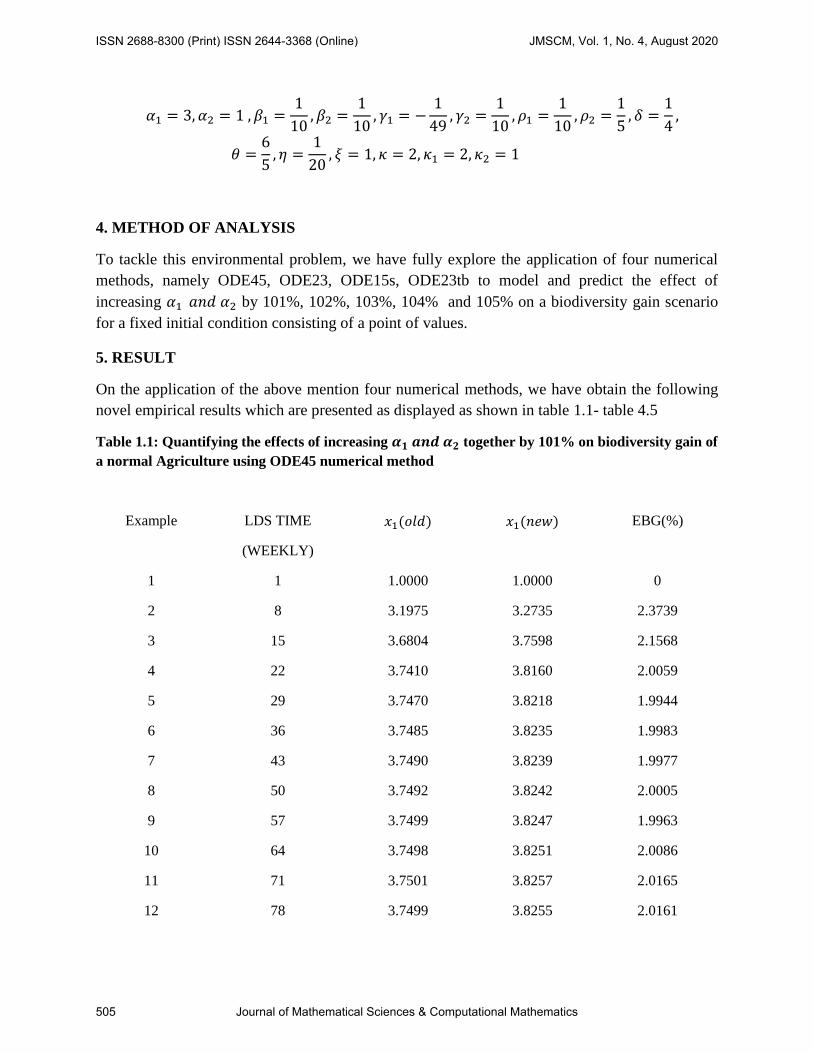
4. METHOD OF ANALYSIS

To tackle this environmental problem, we have fully explore the application of four numerical

methods, namely ODE45, ODE23, ODE15s, ODE23tb to model and predict the effect of

increasing 𝛼1 𝑎𝑛𝑑 𝛼2 by 101%, 102%, 103%, 104% and 105% on a biodiversity gain scenario

for a fixed initial condition consisting of a point of values.

5. RESULT

On the application of the above mention four numerical methods, we have obtain the following

novel empirical results which are presented as displayed as shown in table 1.1- table 4.5

Table 1.1: Quantifying the effects of increasing 𝜶𝟏 𝒂𝒏𝒅 𝜶𝟐 together by 101% on biodiversity gain of

a normal Agriculture using ODE45 numerical method

Example LDS TIME

(WEEKLY)

𝑥1(𝑜𝑙𝑑) 𝑥1(𝑛𝑒𝑤) EBG(%)

1 1 1.0000 1.0000 0

2 8 3.1975 3.2735 2.3739

3 15 3.6804 3.7598 2.1568

4 22 3.7410 3.8160 2.0059

5 29 3.7470 3.8218 1.9944

6 36 3.7485 3.8235 1.9983

7 43 3.7490 3.8239 1.9977

8 50 3.7492 3.8242 2.0005

9 57 3.7499 3.8247 1.9963

10 64 3.7498 3.8251 2.0086

11 71 3.7501 3.8257 2.0165

12 78 3.7499 3.8255 2.0161

ISSN 2688-8300 (Print) ISSN 2644-3368 (Online) JMSCM, Vol. 1, No. 4, August 2020

505 Journal of Mathematical Sciences & Computational Mathematics

13 85 3.7503 3.8255 2.0047

14 92 3.7500 3.8257 2.0192

15 99 3.7498 3.8257 2.0232

16 106 3.7499 3.8259 2.0269

17 113 3.7502 3.8257 2.0138

18 120 3.7501 3.8260 2.0240

19 127 3.7499 3.8259 2.0257

20 134 3.7497 3.8257 2.0293

21 141 3.7501 3.8258 2.0204

LGS= Length of growing season

𝑥1(𝑜𝑙𝑑)= Measures the normal agricultural volume when all model parameters are fixed at 100%

𝑥1(𝑛𝑒𝑤)= Measures the normal agricultural volume when 𝛼1 𝑎𝑛𝑑 𝛼2 only are varied.

EBL= Estimated Biodiversity Gain

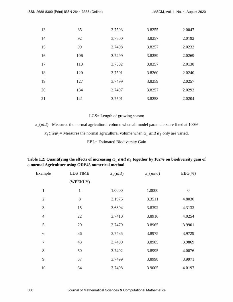
Table 1.2: Quantifying the effects of increasing 𝜶𝟏 𝒂𝒏𝒅 𝜶𝟐 together by 102% on biodiversity gain of

a normal Agriculture using ODE45 numerical method

Example LDS TIME

(WEEKLY)

𝑥1(𝑜𝑙𝑑) 𝑥1(𝑛𝑒𝑤) EBG(%)

1 1 1.0000 1.0000 0

2 8 3.1975 3.3511 4.8030

3 15 3.6804 3.8392 4.3133

4 22 3.7410 3.8916 4.0254

5 29 3.7470 3.8965 3.9901

6 36 3.7485 3.8975 3.9729

7 43 3.7490 3.8985 3.9869

8 50 3.7492 3.8995 4.0076

9 57 3.7499 3.8998 3.9971

10 64 3.7498 3.9005 4.0197

ISSN 2688-8300 (Print) ISSN 2644-3368 (Online) JMSCM, Vol. 1, No. 4, August 2020

506 Journal of Mathematical Sciences & Computational Mathematics

11 71 3.7501 3.9002 4.0027

12 78 3.7499 3.9008 4.0254

13 85 3.7503 3.9010 4.0188

14 92 3.7500 3.9014 4.0370

15 99 3.7498 3.9014 4.0435

16 106 3.7499 3.9013 4.0376

17 113 3.7502 3.9020 4.0489

18 120 3.7501 3.9020 4.0507

19 127 3.7499 3.9023 4.0642

20 134 3.7497 3.9020 4.0638

21 141 3.7501 3.9017 4.0444

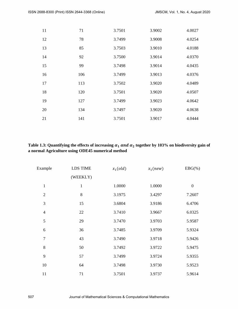
Table 1.3: Quantifying the effects of increasing 𝜶𝟏 𝒂𝒏𝒅 𝜶𝟐 together by 103% on biodiversity gain of

a normal Agriculture using ODE45 numerical method

Example LDS TIME

(WEEKLY)

𝑥1(𝑜𝑙𝑑) 𝑥1(𝑛𝑒𝑤) EBG(%)

1 1 1.0000 1.0000 0

2 8 3.1975 3.4297 7.2607

3 15 3.6804 3.9186 6.4706

4 22 3.7410 3.9667 6.0325

5 29 3.7470 3.9703 5.9587

6 36 3.7485 3.9709 5.9324

7 43 3.7490 3.9718 5.9426

8 50 3.7492 3.9722 5.9475

9 57 3.7499 3.9724 5.9355

10 64 3.7498 3.9730 5.9523

11 71 3.7501 3.9737 5.9614

ISSN 2688-8300 (Print) ISSN 2644-3368 (Online) JMSCM, Vol. 1, No. 4, August 2020

507 Journal of Mathematical Sciences & Computational Mathematics

12 78 3.7499 3.9740 5.9757

13 85 3.7503 3.9743 5.9735

14 92 3.7500 3.9752 6.0060

15 99 3.7498 3.9749 6.0033

16 106 3.7499 3.9750 6.0036

17 113 3.7502 3.9754 6.0054

18 120 3.7501 3.9760 6.0237

19 127 3.7499 3.9757 6.0214

20 134 3.7497 3.9760 6.0359

21 141 3.7501 3.9760 6.0247

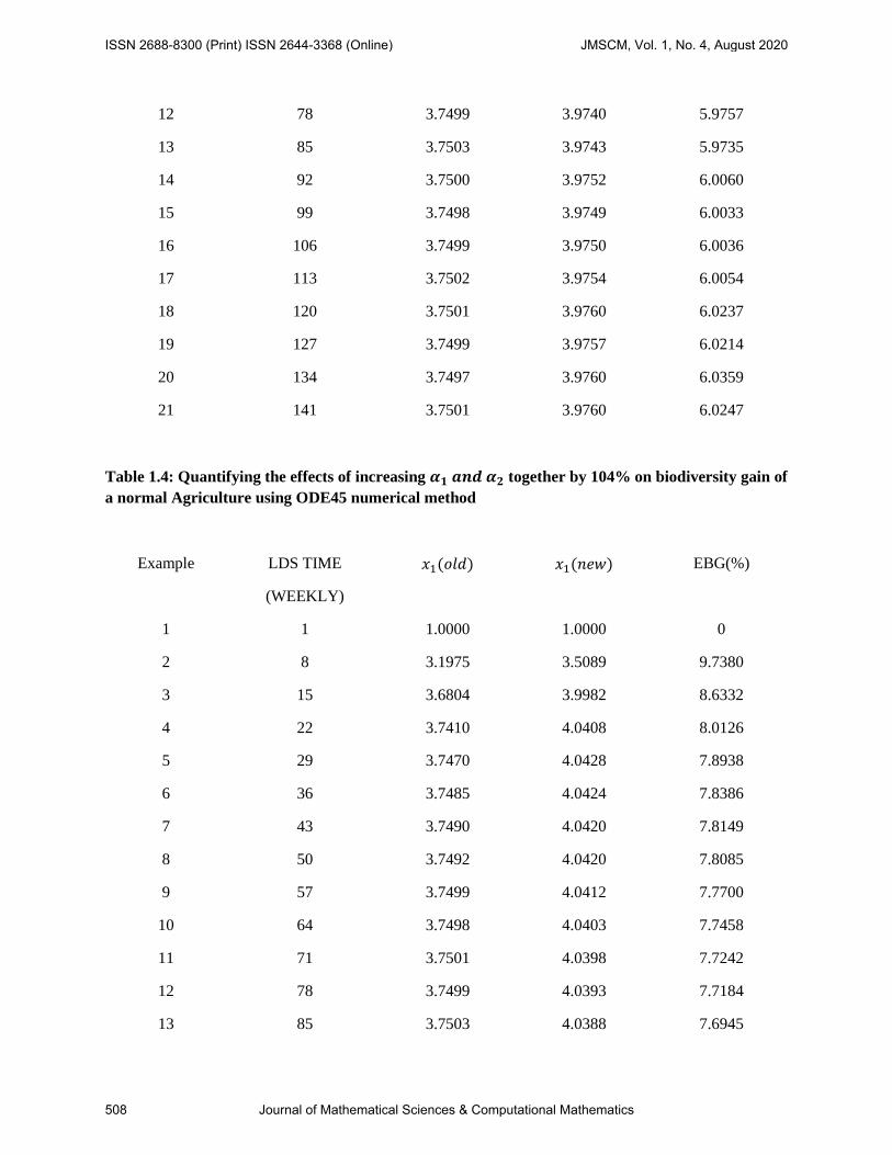
Table 1.4: Quantifying the effects of increasing 𝜶𝟏 𝒂𝒏𝒅 𝜶𝟐 together by 104% on biodiversity gain of

a normal Agriculture using ODE45 numerical method

Example LDS TIME

(WEEKLY)

𝑥1(𝑜𝑙𝑑) 𝑥1(𝑛𝑒𝑤) EBG(%)

1 1 1.0000 1.0000 0

2 8 3.1975 3.5089 9.7380

3 15 3.6804 3.9982 8.6332

4 22 3.7410 4.0408 8.0126

5 29 3.7470 4.0428 7.8938

6 36 3.7485 4.0424 7.8386

7 43 3.7490 4.0420 7.8149

8 50 3.7492 4.0420 7.8085

9 57 3.7499 4.0412 7.7700

10 64 3.7498 4.0403 7.7458

11 71 3.7501 4.0398 7.7242

12 78 3.7499 4.0393 7.7184

13 85 3.7503 4.0388 7.6945

ISSN 2688-8300 (Print) ISSN 2644-3368 (Online) JMSCM, Vol. 1, No. 4, August 2020

508 Journal of Mathematical Sciences & Computational Mathematics

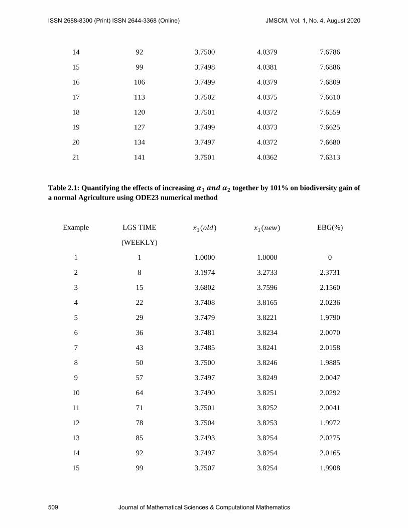
14 92 3.7500 4.0379 7.6786

15 99 3.7498 4.0381 7.6886

16 106 3.7499 4.0379 7.6809

17 113 3.7502 4.0375 7.6610

18 120 3.7501 4.0372 7.6559

19 127 3.7499 4.0373 7.6625

20 134 3.7497 4.0372 7.6680

21 141 3.7501 4.0362 7.6313

Table 2.1: Quantifying the effects of increasing 𝜶𝟏 𝒂𝒏𝒅 𝜶𝟐 together by 101% on biodiversity gain of

a normal Agriculture using ODE23 numerical method

Example LGS TIME

(WEEKLY)

𝑥1(𝑜𝑙𝑑) 𝑥1(𝑛𝑒𝑤) EBG(%)

1 1 1.0000 1.0000 0

2 8 3.1974 3.2733 2.3731

3 15 3.6802 3.7596 2.1560

4 22 3.7408 3.8165 2.0236

5 29 3.7479 3.8221 1.9790

6 36 3.7481 3.8234 2.0070

7 43 3.7485 3.8241 2.0158

8 50 3.7500 3.8246 1.9885

9 57 3.7497 3.8249 2.0047

10 64 3.7490 3.8251 2.0292

11 71 3.7501 3.8252 2.0041

12 78 3.7504 3.8253 1.9972

13 85 3.7493 3.8254 2.0275

14 92 3.7497 3.8254 2.0165

15 99 3.7507 3.8254 1.9908

ISSN 2688-8300 (Print) ISSN 2644-3368 (Online) JMSCM, Vol. 1, No. 4, August 2020

509 Journal of Mathematical Sciences & Computational Mathematics

16 106 3.7498 3.8253 2.0141

17 113 3.7494 3.8253 2.0243

18 120 3.7505 3.8253 1.9932

19 127 3.7503 3.8252 1.9988

20 134 3.7493 3.8252 2.0252

21 141 3.7501 3.8252 2.0031

Table 2.2: Quantifying the effects of increasing 𝜶𝟏 𝒂𝒏𝒅 𝜶𝟐 together by 102% on biodiversity gain of

a normal Agriculture using ODE23 numerical method

Example LGS TIME

(WEEKLY)

𝑥1(𝑜𝑙𝑑) 𝑥1(𝑛𝑒𝑤) EBL(%)

1 1 1.0000 1.0000 0

2 8 3.1974 3.3514 4.8166

3 15 3.6802 3.8399 4.3393

4 22 3.7408 3.8918 4.0368

5 29 3.7479 3.8956 3.9410

6 36 3.7481 3.8978 3.9940

7 43 3.7485 3.8989 4.0126

8 50 3.7500 3.8985 3.9592

9 57 3.7497 3.8998 4.0037

10 64 3.7490 3.9007 4.0460

11 71 3.7501 3.8999 3.9951

12 78 3.7504 3.9010 4.0148

13 85 3.7493 3.9017 4.0635

14 92 3.7497 3.9007 4.0258

15 99 3.7507 3.9017 4.0258

16 106 3.7498 3.9022 4.0649

17 113 3.7494 3.9012 4.0475

ISSN 2688-8300 (Print) ISSN 2644-3368 (Online) JMSCM, Vol. 1, No. 4, August 2020

510 Journal of Mathematical Sciences & Computational Mathematics

18 120 3.7505 3.9021 4.0421

19 127 3.7503 3.9025 4.0593

20 134 3.7493 3.9014 4.0576

21 141 3.7501 3.9024 4.0618

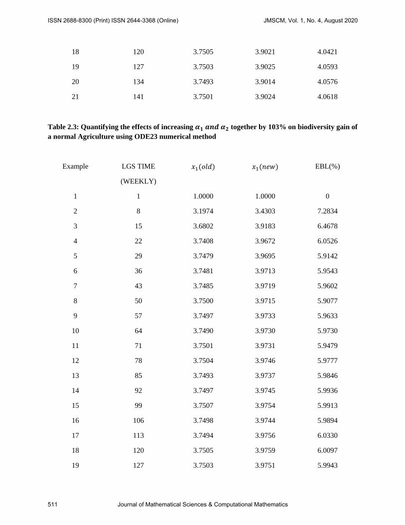
Table 2.3: Quantifying the effects of increasing 𝜶𝟏 𝒂𝒏𝒅 𝜶𝟐 together by 103% on biodiversity gain of

a normal Agriculture using ODE23 numerical method

Example LGS TIME

(WEEKLY)

𝑥1(𝑜𝑙𝑑) 𝑥1(𝑛𝑒𝑤) EBL(%)

1 1 1.0000 1.0000 0

2 8 3.1974 3.4303 7.2834

3 15 3.6802 3.9183 6.4678

4 22 3.7408 3.9672 6.0526

5 29 3.7479 3.9695 5.9142

6 36 3.7481 3.9713 5.9543

7 43 3.7485 3.9719 5.9602

8 50 3.7500 3.9715 5.9077

9 57 3.7497 3.9733 5.9633

10 64 3.7490 3.9730 5.9730

11 71 3.7501 3.9731 5.9479

12 78 3.7504 3.9746 5.9777

13 85 3.7493 3.9737 5.9846

14 92 3.7497 3.9745 5.9936

15 99 3.7507 3.9754 5.9913

16 106 3.7498 3.9744 5.9894

17 113 3.7494 3.9756 6.0330

18 120 3.7505 3.9759 6.0097

19 127 3.7503 3.9751 5.9943

ISSN 2688-8300 (Print) ISSN 2644-3368 (Online) JMSCM, Vol. 1, No. 4, August 2020

511 Journal of Mathematical Sciences & Computational Mathematics

20 134 3.7493 3.9765 6.0601

21 141 3.7501 3.9763 6.0313

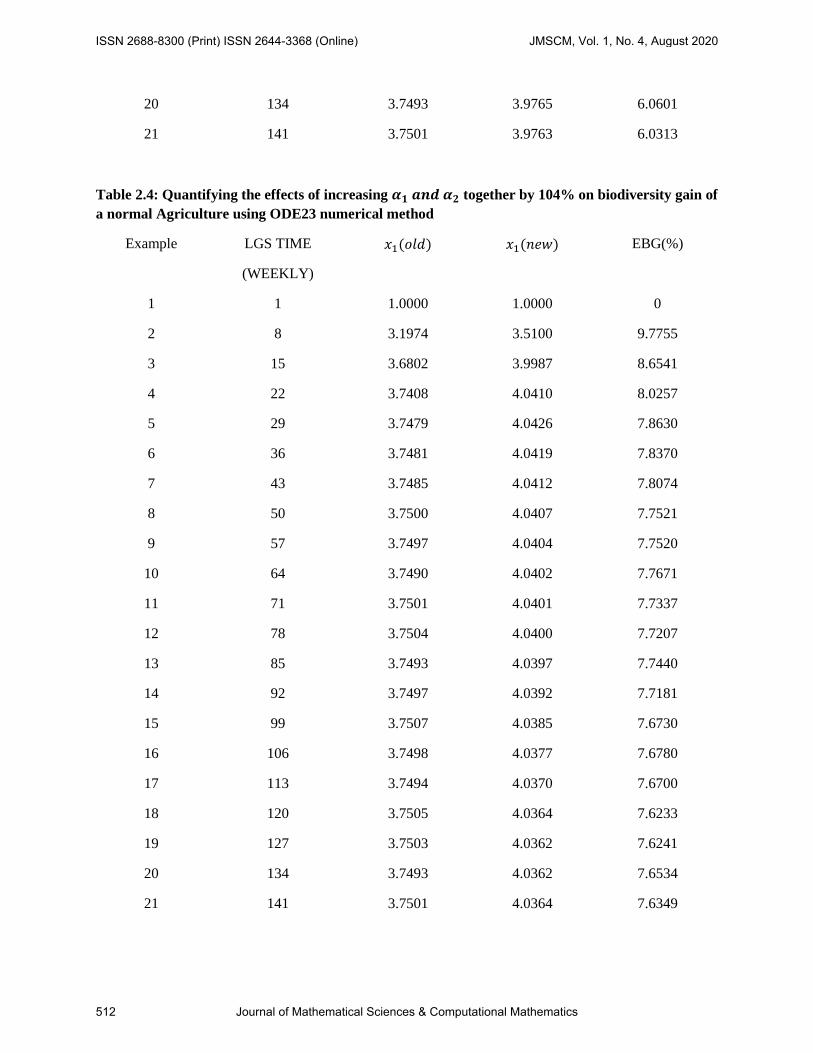
Table 2.4: Quantifying the effects of increasing 𝜶𝟏 𝒂𝒏𝒅 𝜶𝟐 together by 104% on biodiversity gain of

a normal Agriculture using ODE23 numerical method

Example LGS TIME

(WEEKLY)

𝑥1(𝑜𝑙𝑑) 𝑥1(𝑛𝑒𝑤) EBG(%)

1 1 1.0000 1.0000 0

2 8 3.1974 3.5100 9.7755

3 15 3.6802 3.9987 8.6541

4 22 3.7408 4.0410 8.0257

5 29 3.7479 4.0426 7.8630

6 36 3.7481 4.0419 7.8370

7 43 3.7485 4.0412 7.8074

8 50 3.7500 4.0407 7.7521

9 57 3.7497 4.0404 7.7520

10 64 3.7490 4.0402 7.7671

11 71 3.7501 4.0401 7.7337

12 78 3.7504 4.0400 7.7207

13 85 3.7493 4.0397 7.7440

14 92 3.7497 4.0392 7.7181

15 99 3.7507 4.0385 7.6730

16 106 3.7498 4.0377 7.6780

17 113 3.7494 4.0370 7.6700

18 120 3.7505 4.0364 7.6233

19 127 3.7503 4.0362 7.6241

20 134 3.7493 4.0362 7.6534

21 141 3.7501 4.0364 7.6349

ISSN 2688-8300 (Print) ISSN 2644-3368 (Online) JMSCM, Vol. 1, No. 4, August 2020

512 Journal of Mathematical Sciences & Computational Mathematics

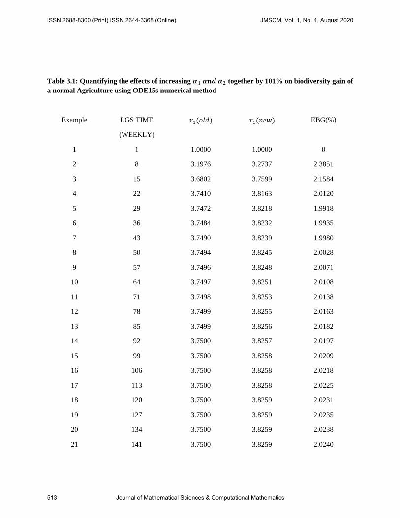
Table 3.1: Quantifying the effects of increasing 𝜶𝟏 𝒂𝒏𝒅 𝜶𝟐 together by 101% on biodiversity gain of

a normal Agriculture using ODE15s numerical method

Example LGS TIME

(WEEKLY)

𝑥1(𝑜𝑙𝑑) 𝑥1(𝑛𝑒𝑤) EBG(%)

1 1 1.0000 1.0000 0

2 8 3.1976 3.2737 2.3851

3 15 3.6802 3.7599 2.1584

4 22 3.7410 3.8163 2.0120

5 29 3.7472 3.8218 1.9918

6 36 3.7484 3.8232 1.9935

7 43 3.7490 3.8239 1.9980

8 50 3.7494 3.8245 2.0028

9 57 3.7496 3.8248 2.0071

10 64 3.7497 3.8251 2.0108

11 71 3.7498 3.8253 2.0138

12 78 3.7499 3.8255 2.0163

13 85 3.7499 3.8256 2.0182

14 92 3.7500 3.8257 2.0197

15 99 3.7500 3.8258 2.0209

16 106 3.7500 3.8258 2.0218

17 113 3.7500 3.8258 2.0225

18 120 3.7500 3.8259 2.0231

19 127 3.7500 3.8259 2.0235

20 134 3.7500 3.8259 2.0238

21 141 3.7500 3.8259 2.0240

ISSN 2688-8300 (Print) ISSN 2644-3368 (Online) JMSCM, Vol. 1, No. 4, August 2020

513 Journal of Mathematical Sciences & Computational Mathematics

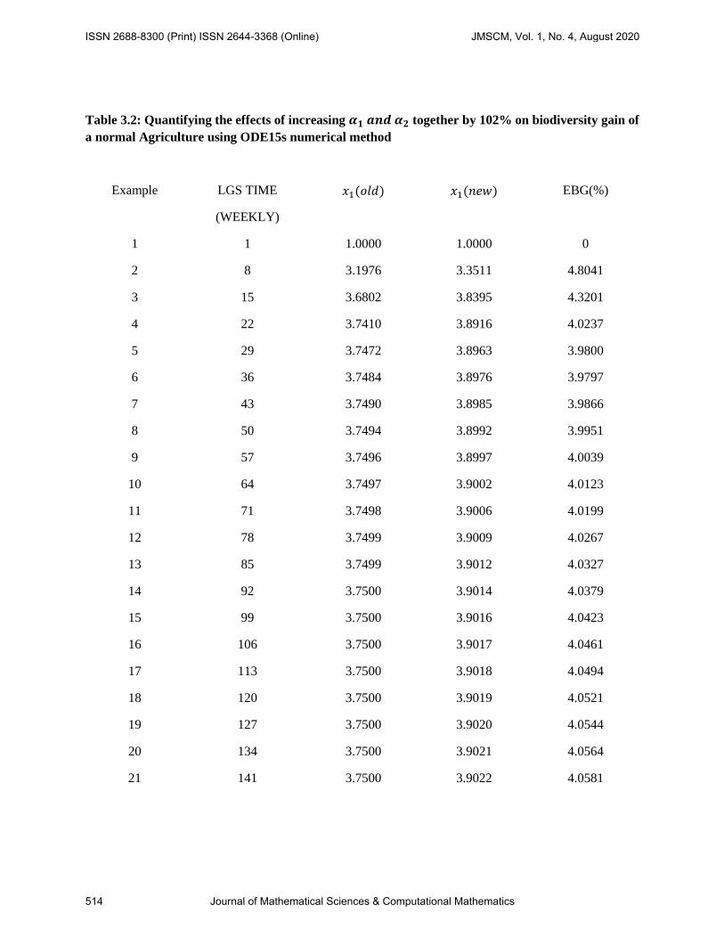
Table 3.2: Quantifying the effects of increasing 𝜶𝟏 𝒂𝒏𝒅 𝜶𝟐 together by 102% on biodiversity gain of

a normal Agriculture using ODE15s numerical method

Example LGS TIME

(WEEKLY)

𝑥1(𝑜𝑙𝑑) 𝑥1(𝑛𝑒𝑤) EBG(%)

1 1 1.0000 1.0000 0

2 8 3.1976 3.3511 4.8041

3 15 3.6802 3.8395 4.3201

4 22 3.7410 3.8916 4.0237

5 29 3.7472 3.8963 3.9800

6 36 3.7484 3.8976 3.9797

7 43 3.7490 3.8985 3.9866

8 50 3.7494 3.8992 3.9951

9 57 3.7496 3.8997 4.0039

10 64 3.7497 3.9002 4.0123

11 71 3.7498 3.9006 4.0199

12 78 3.7499 3.9009 4.0267

13 85 3.7499 3.9012 4.0327

14 92 3.7500 3.9014 4.0379

15 99 3.7500 3.9016 4.0423

16 106 3.7500 3.9017 4.0461

17 113 3.7500 3.9018 4.0494

18 120 3.7500 3.9019 4.0521

19 127 3.7500 3.9020 4.0544

20 134 3.7500 3.9021 4.0564

21 141 3.7500 3.9022 4.0581

ISSN 2688-8300 (Print) ISSN 2644-3368 (Online) JMSCM, Vol. 1, No. 4, August 2020

514 Journal of Mathematical Sciences & Computational Mathematics

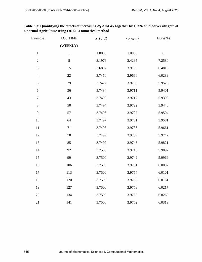
Table 3.3: Quantifying the effects of increasing 𝜶𝟏 𝒂𝒏𝒅 𝜶𝟐 together by 103% on biodiversity gain of

a normal Agriculture using ODE15s numerical method

Example LGS TIME

(WEEKLY)

𝑥1(𝑜𝑙𝑑) 𝑥1(𝑛𝑒𝑤) EBG(%)

1 1 1.0000 1.0000 0

2 8 3.1976 3.4295 7.2580

3 15 3.6802 3.9190 6.4816

4 22 3.7410 3.9666 6.0289

5 29 3.7472 3.9703 5.9526

6 36 3.7484 3.9711 5.9401

7 43 3.7490 3.9717 5.9398

8 50 3.7494 3.9722 5.9440

9 57 3.7496 3.9727 5.9504

10 64 3.7497 3.9731 5.9581

11 71 3.7498 3.9736 5.9661

12 78 3.7499 3.9739 5.9742

13 85 3.7499 3.9743 5.9821

14 92 3.7500 3.9746 5.9897

15 99 3.7500 3.9749 5.9969

16 106 3.7500 3.9751 6.0037

17 113 3.7500 3.9754 6.0101

18 120 3.7500 3.9756 6.0161

19 127 3.7500 3.9758 6.0217

20 134 3.7500 3.9760 6.0269

21 141 3.7500 3.9762 6.0319

ISSN 2688-8300 (Print) ISSN 2644-3368 (Online) JMSCM, Vol. 1, No. 4, August 2020

515 Journal of Mathematical Sciences & Computational Mathematics

Table 3.4: Quantifying the effects of increasing 𝜶𝟏 𝒂𝒏𝒅 𝜶𝟐 together by 104% on biodiversity gain of

a normal Agriculture using ODE15s numerical method

Example LGS TIME

(WEEKLY)

𝑥1(𝑜𝑙𝑑) 𝑥1(𝑛𝑒𝑤) EBG(%)

1 1 1.0000 1.0000 0

2 8 3.1976 3.5091 9.7467

3 15 3.6802 3.9985 8.6408

4 22 3.7410 4.0411 8.0196

5 29 3.7472 4.0430 7.8925

6 36 3.7484 4.0425 7.8454

7 43 3.7490 4.0420 7.8139

8 50 3.7494 4.0414 7.7892

9 57 3.7496 4.0409 7.7687

10 64 3.7497 4.0404 7.7511

11 71 3.7498 4.0399 7.7355

12 78 3.7499 4.0394 7.7216

13 85 3.7499 4.0390 7.7088

14 92 3.7500 4.0386 7.6971

15 99 3.7500 4.0382 7.6863

16 106 3.7500 4.0378 7.6762

17 113 3.7500 4.0375 7.6669

18 120 3.7500 4.0372 7.6582

19 127 3.7500 4.0369 7.6502

20 134 3.7500 4.0366 7.6428

21 141 3.7500 4.0363 7.6359

ISSN 2688-8300 (Print) ISSN 2644-3368 (Online) JMSCM, Vol. 1, No. 4, August 2020

516 Journal of Mathematical Sciences & Computational Mathematics

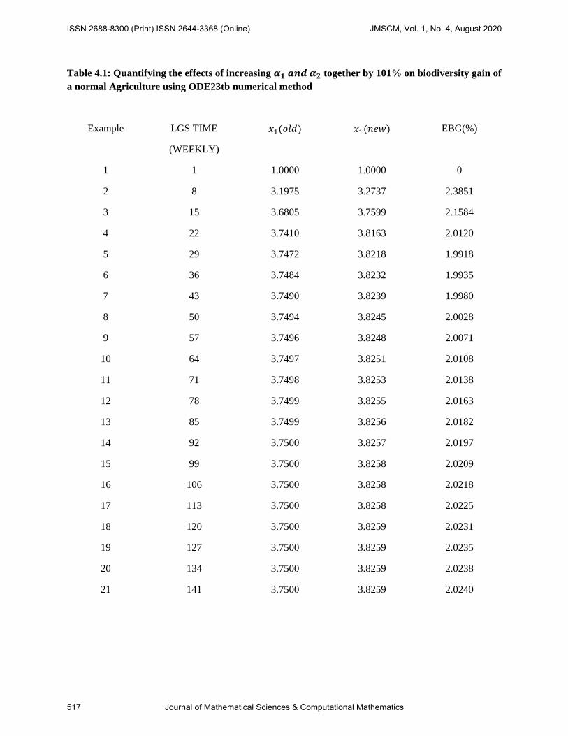
Table 4.1: Quantifying the effects of increasing 𝜶𝟏 𝒂𝒏𝒅 𝜶𝟐 together by 101% on biodiversity gain of

a normal Agriculture using ODE23tb numerical method

Example LGS TIME

(WEEKLY)

𝑥1(𝑜𝑙𝑑) 𝑥1(𝑛𝑒𝑤) EBG(%)

1 1 1.0000 1.0000 0

2 8 3.1975 3.2737 2.3851

3 15 3.6805 3.7599 2.1584

4 22 3.7410 3.8163 2.0120

5 29 3.7472 3.8218 1.9918

6 36 3.7484 3.8232 1.9935

7 43 3.7490 3.8239 1.9980

8 50 3.7494 3.8245 2.0028

9 57 3.7496 3.8248 2.0071

10 64 3.7497 3.8251 2.0108

11 71 3.7498 3.8253 2.0138

12 78 3.7499 3.8255 2.0163

13 85 3.7499 3.8256 2.0182

14 92 3.7500 3.8257 2.0197

15 99 3.7500 3.8258 2.0209

16 106 3.7500 3.8258 2.0218

17 113 3.7500 3.8258 2.0225

18 120 3.7500 3.8259 2.0231

19 127 3.7500 3.8259 2.0235

20 134 3.7500 3.8259 2.0238

21 141 3.7500 3.8259 2.0240

ISSN 2688-8300 (Print) ISSN 2644-3368 (Online) JMSCM, Vol. 1, No. 4, August 2020

517 Journal of Mathematical Sciences & Computational Mathematics

Table 4.2: Quantifying the effects of increasing 𝜶𝟏 𝒂𝒏𝒅 𝜶𝟐 together by 102% on biodiversity gain of

a normal Agriculture using ODE23tb numerical method

Example LGS TIME

(WEEKLY)

𝑥1(𝑜𝑙𝑑) 𝑥1(𝑛𝑒𝑤) EBG(%)

1 1 1.0000 1.0000 0

2 8 3.1975 3.3511 4.8041

3 15 3.6805 3.8395 4.3201

4 22 3.7410 3.8916 4.0237

5 29 3.7472 3.8963 3.9800

6 36 3.7484 3.8976 3.9797

7 43 3.7490 3.8985 3.9866

8 50 3.7494 3.8992 3.9951

9 57 3.7496 3.8997 4.0039

10 64 3.7497 3.9002 4.0123

11 71 3.7498 3.9006 4.0199

12 78 3.7499 3.9009 4.0267

13 85 3.7499 3.9012 4.0327

14 92 3.7500 3.9014 4.0379

15 99 3.7500 3.9016 4.0423

16 106 3.7500 3.9017 4.0461

17 113 3.7500 3.9018 4.0494

18 120 3.7500 3.9019 4.0521

19 127 3.7500 3.9020 4.0544

20 134 3.7500 3.9021 4.0564

21 141 3.7500 3.9022 4.0581

ISSN 2688-8300 (Print) ISSN 2644-3368 (Online) JMSCM, Vol. 1, No. 4, August 2020

518 Journal of Mathematical Sciences & Computational Mathematics

Table 4.3: Quantifying the effects of increasing 𝜶𝟏 𝒂𝒏𝒅 𝜶𝟐 together by 103% on biodiversity gain of

a normal Agriculture using ODE23 numerical method

Example LGS TIME

(WEEKLY)

𝑥1(𝑜𝑙𝑑) 𝑥1(𝑛𝑒𝑤) EBG(%)

1 1 1.0000 1.0000 0

2 8 3.1975 3.4295 7.2580

3 15 3.6805 3.9190 6.4816

4 22 3.7410 3.9666 6.0289

5 29 3.7472 3.9703 5.9526

6 36 3.7484 3.9711 5.9401

7 43 3.7490 3.9717 5.9398

8 50 3.7494 3.9722 5.9440

9 57 3.7496 3.9727 5.9504

10 64 3.7497 3.9731 5.9581

11 71 3.7498 3.9736 5.9661

12 78 3.7499 3.9739 5.9742

13 85 3.7499 3.9743 5.9821

14 92 3.7500 3.9746 5.9897

15 99 3.7500 3.9749 5.9969

16 106 3.7500 3.9751 6.0037

17 113 3.7500 3.9754 6.0101

18 120 3.7500 3.9756 6.0161

19 127 3.7500 3.9758 6.0217

20 134 3.7500 3.9760 6.0269

21 141 3.7500 3.9762 6.0319

ISSN 2688-8300 (Print) ISSN 2644-3368 (Online) JMSCM, Vol. 1, No. 4, August 2020

519 Journal of Mathematical Sciences & Computational Mathematics

Table 4.4: Quantifying the effects of increasing 𝜶𝟏 𝒂𝒏𝒅 𝜶𝟐 together by 104% on biodiversity gain of

a normal Agriculture using ODE23tb numerical method

Example LGS TIME

(WEEKLY)

𝑥1(𝑜𝑙𝑑) 𝑥1(𝑛𝑒𝑤) EBG(%)

1 1 1.0000 1.0000 0

2 8 3.1975 3.5091 9.7467

3 15 3.6805 3.9985 8.6408

4 22 3.7410 4.0411 8.0196

5 29 3.7472 4.0430 7.8925

6 36 3.7484 4.0425 7.8454

7 43 3.7490 4.0420 7.8139

8 50 3.7494 4.0414 7.7892

9 57 3.7496 4.0409 7.7687

10 64 3.7497 4.0404 7.7511

11 71 3.7498 4.0399 7.7355

12 78 3.7499 4.0394 7.7216

13 85 3.7499 4.0390 7.7088

14 92 3.7500 4.0386 7.6971

15 99 3.7500 4.0382 7.6863

16 106 3.7500 4.0378 7.6762

17 113 3.7500 4.0375 7.6669

18 120 3.7500 4.0372 7.6582

19 127 3.7500 4.0369 7.6502

20 134 3.7500 4.0366 7.6428

21 141 3.7500 4.0363 7.6359

ISSN 2688-8300 (Print) ISSN 2644-3368 (Online) JMSCM, Vol. 1, No. 4, August 2020

520 Journal of Mathematical Sciences & Computational Mathematics

6. RESULTS & DISCUSSION

In this paper, we have applied a mathematical model to discuss and predict the growth of normal

agricultural assets by comparing four differential methods of ordinary differential equation

(ODE45, ODE23, ODE15s, and ODE23tb). From the result obtained, we have seen that the growth

of normal agricultural assets depends on time and the normal agricultural assets changes

deterministically as the length of growing season changes where all the model parameter values

are fixed, however when the model value 𝛼1 𝑎𝑛𝑑 𝛼2 are increase 101%-104%, the normal

agricultural variable also changes. From the numerical prediction using four method of ODE which

are similar, ODE45 appears to be more efficient than the others. Applying these four methods, we

have seen that the pattern of growth of these two interacting normal agricultural data have finite

instance of biodiversity.

REFERENCES

[1] I. Agyemang, H.I. Freedman, J.W. Macki, An ecospheric recovery model for agriculture industry

interactions, Diff. Eqns. Dyn. Syst. 15 (2007) 185-208.

[2] I. Agyemang, H.I. Freedman, An environmental model for the interaction of industry with two

competing agricultural resource, Elsevier. 49(2009) 1618-16

[3] H. Amman, Ordinary Differential Equations: Introduction to Non-Linear Analysis, Walter de Gruyter,

Berlin, 1990.

[4] A.G Eleki, R.E Akpodee and E.N Ekakaa, The differential effects of a scenario of a non-additive

environmental perturbation on biodiversity ecospheric assets: Kalabari kingdom of ecospheric assets,

African Publication and research international, 2019 1-15

[5] A.G Eleki and E.N Ekakaa, Computational Modelling of ecosperic assets: alternative numerical

approach, African Scholar publications and research international, 15(2), 2019, 160-165

[6] L.P. Apedaile, H.I. Freedman, S.G.M. Schilizzi, M. Solomonovich, Equilibria and dynamics in an

economic predator prey model of agriculture, Math. Comput. Model. 19 (1994) 1 -15.

[7] G.J. Butler, H.I. Freedman, P.E. Waltman, Uniformly persistent systems, Proc. Amer. Math. Soc. 96

(1986) 425 430.

[8] Michael A. Obe, Godspower C. Abanum, Innocent C. Eli, Variational Iteration Method for first and

second ordinary differential equation using first kind chebychev polynomials, IJASRE. 4(2018) 126-130

[9] Godspower C.A, Charles O and Ekakaa E.N, Numerical Simulation of biodiversity Loss: Comparison

of numerical methods,IJMTT. 66(2020) 53-64

ISSN 2688-8300 (Print) ISSN 2644-3368 (Online) JMSCM, Vol. 1, No. 4, August 2020

521 Journal of Mathematical Sciences & Computational Mathematics

[10] G.J. Butler, P. Waltman, Persistence in three-dimensional Lotka Volterra systems, Math. Comput.

Model. 10 (1988) 13 16.

[11] C.W. Clark, Mathematical Bioeconomics: The Optimal Management of Renewable Resources, Wiley,

New York, 1990.

[12] G.C. Daily, Natures Services: Societal Dependence on Natural Ecosystem, Island Press, Washington,

DC, 1997.

[13] G.C. Daily, K. Ellison, The New Economy of Nature: The Quest to Make Conservation Profitable,

Island Press, Washington, DC, 2002.

[14] G.C. Daily, P.A. Matson, P.M. Vitousek, Ecosystem services supplied by soil, in: Natures Services:

Societal Dependence on Natural Ecosystem, Island Press, Washington, DC, 1997.

[15] L. Edelstein-Keshet, Mathematical Models in Biology, Random House, New York, 1988.

[16] H.W. Eves, Foundations and Fundamental Concepts of Mathematics, PWS-Kent, Boston, 1990.

[17] H.I. Freedman, Deterministic Mathematical Models in Population Ecology, Marcel Dekker Inc., New

York, 1980.

[18] H.I. Freedman, P. Moson, Persistence definitions and their connections, Proc. Amer. Math. Soc. 109

(1990) 1025 1033.

[19] H.I. Freedman, J.W.-H. So, Global stability and persistence of simple food chains, Math. Biosci. 73

(1985) 89 91.

[20] H.I. Freedman, M. Solomonovich, L.P. Apedaile, A. Hailu, Stability in models of agricultural-industry-

environment interactions, in: Advances in Stability Theory, vol. 13, Taylor and Francis, London, 2003, pp.

255 265.

[21] H.I. Freedman, P. Waltman, Persistence in a model of three competitive populations, Math. Biosci. 73

(1985) 89 91.

[22] H.I. Freedman, P. Waltman, Persistence in a model of three interacting predator-prey populations,

Math. Biosci. 68 (1984) 213 231.

[23] G. Heal, Nature and the Marketplace: Capturing the Value of Ecosystem Services, Island Press,

Washington, DC, 2000.

[24] L. Horrigan, R.S. Lawrence, P. Walker, How sustainable agriculture can address the environmental

and human health harms of industrial agriculture, Environ. Health Persp. 110: 445 456.

ISSN 2688-8300 (Print) ISSN 2644-3368 (Online) JMSCM, Vol. 1, No. 4, August 2020

522 Journal of Mathematical Sciences & Computational Mathematics

[25] J. Ikerd, The ecology of sustainability, University of Missouri, MO, USA.

[26] J. Ikerd, Sustaining the profitability of agriculture, Paper presented at extension pre-conference, The

economists role in the agricultural sustainability paradigm, San Antonio, TX, 1996.

[27] M. Solomonovich, L.P. Apedaile, H.I. Freedman, A.H. Gebremedihen, S.M.G. Belostotski, Dynamical

economic model of sustainable agriculture and the ecosphere, Appl. Math. Comput. 84 (1997) 221 246.

[28] M. Solomonovich, L.P. Apedaile, H.I. Freedman, Predictability and trapping under conditions of

globalization of agricultural trade: An application of the CGS approach, Math. Comput. Model. 33 (2001)

495 516.

[29] M. Solomonovich, H.I. Freedman, L.P. Apedaile, S.G.M. Schilizzi, L. Belostotski, Stability and

bifurcations in an environmental recovery model of economic agriculture-industry interactions, Natur.

Resource Modeling 11 (1998) 35 79.

[30] M.L Jhingan, The economics of development and planning, 39th revised and enlarged edition

[31] M. Donatelli, R.D Magarey, S Bregagho, L. Willocquet, J.P.M Whish and S. Savary, Modelling the

impacts of pests and diseases on agricultural systems, Elseavier, agricultural system, 155(2017) 213-224

ISSN 2688-8300 (Print) ISSN 2644-3368 (Online) JMSCM, Vol. 1, No. 4, August 2020

523 Journal of Mathematical Sciences & Computational Mathematics