COMBINATORIAL HARMONIC MAPS AND CONVERGENCE TO

CONFORMAL MAPS, I: A HARMONIC CONJUGATE.

SA’AR HERSONSKY

Abstract. In this paper, we provide new discrete uniformization theorems for bounded,m-connected planar domains. To this end, we consider a planar, bounded, m-connecteddomain Ω, and let ∂Ω be its boundary. Let T denote a triangulation of Ω ∪ ∂Ω. Weconstruct a new decomposition of Ω ∪ ∂Ω into a finite union of quadrilaterals with disjointinteriors. The construction is based on utilizing a pair of harmonic functions on T (0) andproperties of their level curves. In the sequel [26], it will be proved that a particular discretescheme based on these theorems converges to a conformal map, thus providing an affirmativeanswer to a question raised by Stephenson [40, Section 11].

0. Introduction

0.1. Perspective. The Uniformization Theorem for surfaces says that any simply connectedRiemann surface is conformally equivalent to one of three known Riemann surfaces: theopen unit disk, the complex plane or the Riemann sphere. This remarkable theorem isa vast generalization of the celebrated Riemann Mapping Theorem asserting that a non-empty simply connected open subset of the complex plane (which is not the whole of it) isconformally equivalent to the open unit disk.

Our work in this paper is motivated by the following fundamental questions:

Given a topological surface endowed with some combinatorial data, such as a triangulation,can one use the combinatorics and the topology to obtain an effective version of uniformiza-tion theorems, or other types of uniformization theorems?

The nature of the input suggests that one should first prove discrete uniformization theo-rems, i.e., first provide a rough approximation to the desired uniformization map and target.Experience shows that this step is not easy to establish, since the input is coarse in nature(such as a triangulation of the domain), and the output should consist of a map from thedomain to a surface endowed with some kind of a geometric structure.

Ideally, the approximating maps should have nice properties and if this step is successfullycompleted, one then tries to prove convergence of these maps and the output objects attained,under suitable conditions, to concrete geometric objects.

Let us describe two examples exploiting the usefulness of such an approach (see for instance[32] and [20] for other important results). A beautiful and classical result which was firstproved by Koebe [30], The Discrete Circle Packing Theorem, states:

Date: March 14, 2014.2000 Mathematics Subject Classification. Primary: 53C43; Secondary: 57M50, 39A12, 30G25.Key words and phrases. planar networks, harmonic functions on graphs, flat surfaces with conical singu-

larities, discrete uniformization theorems.1

2 SA’AR HERSONSKY

Given a finite planar graph (without multiple edges or loops), there exists a packing ofEuclidean disks in the plane, enumerated by the vertices of the graph, such that the contactgraph of the packing looks exactly like the given graph, that is, the two graphs are isomorphic.

This theorem was later rediscovered by Thurston [42, Chapter 13] as a consequence of An-dreev’s Theorem [2, 3] concerning hyperbolic polyhedra in terms of circles on the Riemannsphere. Thurston envisioned [41] a remarkable application to the theory of conformal map-ping of the complex plane and the Riemann sphere. Thurston conjectured that a discretescheme based on the Discrete Circle Packing Theorem converges to the Riemann mapping.The conjecture which was proved in 1987 by Rodin and Sullivan [35] provides a refreshinggeometric view on Riemann’s Mapping Theorem.

Thurston suggested to Schramm to study the case where the sets in the plane that formthe tiles in the packing are squares. This resulted in The Finite Riemann Mapping Theoremwhich was proved by Schramm [37] and independently by Cannon, Floyd and Parry [13], inthe period 1986–1991:

Let T be a triangulation of a topological planar quadrilateral. Then there is a tiling of arectangle by squares, indexed by the vertices of T , such that the contact graph of the packinglooks exactly like the given graph, that is, the two graphs are isomorphic.

The problem of tiling a rectangle by squares, as provided by the theorem above, is insome sense a discrete analogue of finding a conformal map from a given quadrilateral to arectangle (taking corners to corners and boundary to boundary). In this scheme, each vertexis expanded to a square, the width of the square is a rough estimate to the magnitude ofthe derivative of the uniformizing analytic map at that vertex. In [13] and in [37], it wasproved that all the information which is required to get the square tiling above, is given by asolution of an extremal problem which is a discrete analogue of the notion of extremal lengthfrom complex analysis.

The actual theorem proved by Cannon, Floyd and Parry ([13, Theorem 3.0.1]) is a bitdifferent and slightly more general than the one stated above. Their solution is also basedon discrete extremal length arguments. Another proof of an interesting generalization of [37]was given by Benjamini and Schramm [9] (see also [10] for a related study).

The theme of realizing a given combinatorial object by a packing of concrete geometricobjects has a fascinating history which pre-dated Koebe. In 1903, Dehn [17] showed a relationbetween square tilings and electrical networks. Later on, in the 1940’s, Brooks, Smith, Stoneand Tutte explored a foundational correspondence between a square tiling of a rectangle anda planar multigraph with two poles, a source and a sink [11]. In 1996, Kenyon generalizedDehn’s construction and established a correspondence between certain planar non-reversibleMarkov chains and trapezoid tilings of a rectangle [28].

In [24] and [25], we addressed (using methods that transcend Dehn’s idea) the case wherethe domain has higher connectivity. These papers provide the first step towards an approxi-mation of conformal maps from such domains onto a certain class of flat surfaces with conicalsingularities.

0.2. Motivation and the main ideas of this paper. In his attempts to prove uniformiza-tion, Riemann suggested considering a planar annulus as made of a uniform conducting metalplate. When one applies voltage to the plate, keeping one boundary component at voltage k

A HARMONIC CONJUGATE 3

and the other at voltage 0, electrical current will flow through the annulus. The equipoten-tial lines form a family of disjoint simple closed curves foliating the annulus and separatingthe boundary curves. The current flow lines consist of simple disjoint arcs connecting theboundary components, and they foliate the annulus as well. Together, the two families pro-vide “rectangular” coordinates on the annulus that turn it into a right circular cylinder, ora (conformally equivalent) circular concentric annulus.

In this paper, we will follow Riemann’s perspective on uniformization by constructing“rectangular” coordinates from given combinatorial data. The foundational modern theoryof boundary value problems on graphs enables us to provide a unified framework to thediscrete uniformization theorems mentioned above, as well as to more general situations.The important work of Bendito, Carmona and Encinas (see for instance [6],[7] and [8]) isessential for our applications, and parts of it were utilized quite frequently in [23], [24], [25],this paper, and its sequel [26].

Consider a planar, bounded, m-connected domain Ω, and let ∂Ω be its boundary whichcomprises Jordan curves. Henceforth, let T denote a triangulation of Ω ∪ ∂Ω. We will con-struct a new decomposition of Ω∪∂Ω into R, a finite union of piecewise-linear quadrilateralswith disjoint interiors. We will show that the set of quadrilaterals can be endowed with afinite measure thought of as a combinatorial analogue of the Euclidean planar area measure.

Next, we construct a pair (SΩ, f) where SΩ is a special type of a genus 0, singular flatsurface, having m boundary components, which is tiled by rectangles and is endowed withµ, the canonical area measure induced by the singular flat structure. The map f is ahomeomorphism from (Ω, ∂Ω) onto SΩ. Furthermore, each quadrilateral is mapped to asingle rectangle, and its measure is preserved.

The proof that f is a homeomorphism, as well as the construction of a measure on thespace of quadrilaterals, depends in a crucial way on the existence of a pair of harmonicfunctions on T (0), and a few properties of their level curves.

The motivation for this paper is two fold. First, recall that in the theorems proved in [24](as well as in [25]), the analogous mapping to f was proved to be an energy-preserving map(in a discrete sense) from T (1) onto a particular singular flat surface. Hence, it is not possibleto extend that map to a homeomorphism defined on the domain. Furthermore, the naturalinvariant measure considered there is one-dimensional (being concentrated on edges). Sothat measure is not the one which we expect to converge, as the triangulations get finer, tothe planar Lebesgue measure.

Second, it is shown in [37, page 117] that if one attempts to use the combinatorics ofthe hexagonal lattice, square tilings (as provided by Schramm’s method) cannot be used asdiscrete approximations for the Riemann mapping. There is still much effort by Cannon,Floyd and Parry to provide sufficient conditions under which their method will converge toa conformal map in the cases of an annulus or a quadrilateral.

Thus, the outcome of this paper is the construction of one approximating map to a con-formal map from Ω. In [26], which heavily relies on our work in this paper, we will showthat a scheme of refining the triangulation, coupled with a particular choice of a conduc-tance function in each step (see Section 1.1 for the definition), leads to convergence of themappings constructed in each step, to a canonical conformal mapping from the domain onto

4 SA’AR HERSONSKY

a particular flat surface with conical singularities. This will, in particular, answer a questionraised by Stephenson in 1996 [40, Section 11].

0.3. The results in this paper. We now turn to a more detailed description of this paper.In order to ease the notation and to follow the logic of the various constructions, let usfocus on the case of an annulus. A slit in an annulus is a fixed, simple, combinatorial pathin T (1), along which g is monotone increasing which joins the two boundary components(Definition 2.1).

Let g denote the solution of a discrete Dirichlet boundary value problem defined on T (0)

(see Definition 1.6). We will start by extending g to the interior of the domain: affinely overedges in T (1) and over triangles T (2). We will often abuse notation and will not distinguishbetween a function defined on T (0) and its extension over |T |.

For the applications of this paper and its sequel [26], first in creating “rectangular” coordi-nates in a topological sense, and second in [26] to prove convergence of the maps constructedin Theorem 0.5 and Theorem 5.4 to conformal maps, it is necessary to introduce a newfunction denoted by h on T (0). This function will be defined on an annulus minus a slit (i.e,a quadrilateral) and will be called the harmonic conjugate function; h is the solution of aparticular Dirichlet-Neumann boundary value problem.

In fact, another function g∗ must first be constructed. This function will have the samedomain as h and will be called the conjugate function of g. It is obtained by integrating (ina discrete sense) the normal derivative of g along its level curves (Definition 1.1). Whereasthe normal derivative of g is initially defined only at vertices that belong to ∂Ω, the simpletopological structure of the level curves of g permits the extension of the normal derivativeto the interior, and thereafter its integration. These level curves are simple, piecewise-linear, closed curves that separate the two boundary components and foliate the annulus.Definition 2.6 will formalize this discussion.

There is a technical difficulty in this construction (and others appearing in this paper) if apair of adjacent vertices of T (0) has the same g-values. One may generalize the definitions andthe appropriate constructions, as one solution. For a discussion of this approach and others,see [28, Section 5]. Experimental evidence shows that in the case that the triangulation iscomplicated enough such equality rarely happens. Henceforth in this paper, we will assumethat no pair of adjacent vertices has the same g-values (unless they belong to the sameboundary component).

The analysis of the level curves of g∗ is the subject of Proposition 2.21. Their interactionwith the level curves of g is described in Proposition 2.22. The level curves of g form apiecewise-linear analogue of the level curves of the smooth harmonic function u(r, φ) = r,and those of h form a piecewise-linear analogue of the level curves of the smooth harmonicfunction v(r, φ) = φ.

For any function defined on T (0), and any t ∈ R, we let lt denote the level curve of itsaffine extension corresponding to the value t.

Definition 0.1 (Combinatorial orthogonal filling pair of functions). Let (Ω, ∂Ω, T ) be given,where Ω is an annulus minus a slit. A pair of non-negative functions φ and ψ defined onT (0) will be called combinatorially orthogonal filling, if for any two level curves lα and lβ of

A HARMONIC CONJUGATE 5

φ and ψ, respectively, one has

(0.2) |lα ∩ lβ| = 1,

where | · | denotes the number of intersection points between lα and lβ. Furthermore, it isrequired that each one of the families of level curves is a non-singular foliation of (Ω, ∂Ω, T ).

Note that level curves are computed with respect to the affine extensions of φ and ψ,respectively.

By a simple quadrilateral, we will mean a triangulated, closed topological disk with achoice of four distinct vertices on its boundary. It follows that a combinatorial orthogonalfilling pair of functions induces a cellular decomposition R of Ω ∪ ∂Ω such that each 2-cellis a simple quadrilateral, and each 1-cell is included in a level curve of φ or of ψ. Such adecomposition will be called a rectangular combinatorial net.

We now record the essential properties of the pair g, h in Ω, an annulus minus a slit.

Theorem 0.3. Assume that for every ǫ > 0, every leaf of g is ǫ-close to a leaf of h∗, whereh∗ is the conjugate function of h (Definition 3.4). Then the pair g, h is combinatoriallyorthogonal filling.

Remark 0.4. The metric which we consider is the Gromov-Hausdorff metric. The assumptionwill make the construction of the rectangular net described below easier to carry. In [26], wewill show how to modify our construction once this assumption is removed.

We now turn to stating one of our main discrete uniformization theorems. In the courseof the proofs of our main theorems, we will first construct a new decomposition of Ω into arectangular net, R (Definition 3.15), it is induced by the pair g, h; then a model surfacewhich is, when m > 2, a singular flat surface tiled by rectangles. Finally, we will constructa map between the domain and the model surface and describe its properties.

Let us start with the fundamental case, an annulus. Given two positive real numbers r1and r2, and two angles φ1, φ2 ∈ [0, 2π), the bounded domain in the complex plane whoseboundary is determined by the two circles, u(r, φ) = r1, and u(r, φ) = r2, and the two radialcurves v(r, φ) = φ1, and v(r, φ) = φ2, will be called an annular shell. Let µ denote Lebesguemeasure in the plane. In the statement of the next theorem, the measure ν which is describedin Definition 4.1 is determined by g, g∗ and h. The quantity period(g∗) is an invariant ofg∗ which encapsulates integration of the normal derivative of g along its level curves (seeDefinition 2.19).

Our first discrete uniformization theorem is:

Theorem 0.5 (A discrete Dirichlet problem on an annulus). Let A be a planar annulusendowed with a triangulation T , and let ∂A = E1 ⊔ E2. Let k be a positive constant andlet g be the solution of the discrete Dirichlet boundary value problem defined on (A, ∂A, T )(Definition 1.6).

Let SA be the concentric Euclidean annulus with its inner and outer radii satisfying

(0.6) r1, r2 = 1, 2π exp( 2π

period(g∗)k)

.

Then there exist

6 SA’AR HERSONSKY

(1) a tiling T of SA by annular shells,(2) a homeomorphism

f : (A, ∂A,R) → (SA, ∂SA, T ),

such that f is boundary preserving, it maps each quadrilateral in R(2) onto a singleannular shell in SA; furthermore, f preserves the measure of each quadrilateral, i.e.,

ν(R) = µ(f(R)), for all R ∈ R(2).

The dimensions of each annular shell in the tiling are determined by the boundary valueproblem (in a way that will be described later). In our setting, boundary preserving meansthat the annular shell associated to a quadrilateral in R with an edge on ∂Ω will have anedge on a corresponding boundary component of SA.

Our second discrete uniformization theorem is Theorem 5.4 which provides a geometricmapping and a model for the case m > 2. The model surface that generalizes the concentricannulus in the previous theorem first appeared in [24]. It is a singular flat, genus 0, compactsurface with m > 2 boundary components endowed with finitely many conical singularities.Each cone singularity is an integer multiple of π/2. Such a surface is called a ladder ofsingular pairs of pants.

In order to prove this theorem, we first construct a topological decomposition of Ω intosimpler components; these are annuli and annuli with one singular boundary component, forwhich the previous theorem and a slight generalization of it may be applied. The secondstep of the proof is geometric. We show that it is possible to glue the different componentswhich share a common boundary in a length preserving way. This step entails a new notionof length which is the subject of Definition 3.19.

0.4. Organization of the paper. From [24], we use the description of the topological prop-erties of singular level curves of the Dirichlet boundary value problem. The most significantone is a description of the topological structure of the connected components of any singularlevel curve of the solution. A study of the topology and geometry of the associated levelcurves and their complements is carried out in [24, Section 2]. From [25], we use the descrip-tion of the topological properties of level curves of the Dirichlet-Neumann boundary valueproblem on a quadrilateral. A modest familiarity with [24, 25] will be useful for reading thispaper.

For the purpose of making this paper self-contained, a few basic definitions and some no-tations are recalled in Section 1, and results from [24, 25] are quoted as needed. In Section 2,the first main tool of this paper, a conjugate function to g is defined. In Section 3, the secondmain tool of this paper, a harmonic conjugate function and thereafter a rectangular net, areconstructed on an annulus minus a slit. In Section 4, the cases of an annulus and an annuluswith one singular boundary component are treated, respectively, by Theorem 0.5 and Propo-sition 4.22. Due to the reasons we mentioned in the paragraph preceding this subsection,these are foundational for the applications of this paper and of [26] as well. Section 5 isdevoted to the proof of Theorem 5.4.

Convention. In this paper, we will assume that a fixed affine structure is imposed on(Ω, ∂Ω, T ). The existence of such a structure is obtained by using normal coordinates on

A HARMONIC CONJUGATE 7

(Ω, ∂Ω, T ) (see [39, Theorem 5-7]). Since our methods depend on the combinatorics of thetriangulation, the actual chosen affine structure is not important.

Acknowledgement. It is a pleasure to thank Ted Shifrin and Robert Varley for enjoyableand inspiring discussions related to the subject of this paper. Rich Schwartz graciouslyhelped in formulating the assumption in Theorem 0.3 and in showing its importance. Weare indebted to Bill Floyd and the referee, for their careful reading, comments, corrections,and questions leading to significant improvements on earlier versions of this paper.

1. Finite networks and boundary value problems

In this section, we briefly review classical notions from harmonic analysis on graphsthrough the framework of finite networks. We then describe a procedure to modify a givenboundary problem and T . The reader who is familiar with [24] or [25] may skip to the nextsection.

1.1. Finite networks. In this paragraph, we will mostly be using the notation of Section2 in [5]. Let Γ = (V,E, c) be a planar finite network; that is, a planar, simple, and finiteconnected graph with vertex set V and edge set E, where each edge (x, y) ∈ E is assigned aconductance c(x, y) = c(y, x) > 0. Let P(V ) denote the set of non-negative functions on V .Given F ⊂ V , we denote by F c its complement in V . Set P(F ) = u ∈ P(V ) : S(u) ⊂ F,where S(u) = x ∈ V : u(x) 6= 0. The set δF = x ∈ F c : (x, y) ∈ E for some y ∈ F iscalled the vertex boundary of F . Let F = F ∪ δF , and let E = (x, y) ∈ E : x ∈ F. LetΓ(F ) = (F , E, c) be the network such that c is the restriction of c to E. We write x ∼ y if(x, y) ∈ E.

The following operators are discrete analogues of classical notions in continuous potentialtheory (see for instance [19] and [15]).

Definition 1.1. Let u ∈ P(F ). Then for x ∈ F , the function

(1.2) ∆u(x) =∑

y∼x

c(x, y) (u(x)− u(y))

is called the Laplacian of u at x. For x ∈ δ(F ), let y1, y2, . . . , ym ∈ F be its neighborsenumerated clockwise. The normal derivative of u at a point x ∈ δF with respect to a setF is

(1.3)∂u

∂n(F )(x) =

∑

y∼x, y∈F

c(x, y)(u(x)− u(y)).

Finally, u ∈ P(F ) is called harmonic in F ⊂ V if ∆u(x) = 0, for all x ∈ F .

1.2. Harmonic analysis and boundary value problems on graphs. Consider a pla-nar, bounded, m-connected region Ω, and let ∂Ω be its boundary (m > 1). Let T be atriangulation of Ω ∪ ∂Ω. Let ∂Ω = E1 ∪ E2, where E1 and E2 are disjoint, and E1 is theoutermost component of ∂Ω. Invoke a conductance function C on T (1), thus making it afinite network, and use it to define the Laplacian on T (0).

Notation 1.4. Henceforth, for any F ⊂ V and g : F → R, we let∫

v∈Fg(v) denote

∑

v∈F g(v).

Similarly, for any X ⊂ E and h : X → R, we let∫

e∈Xh(e) denote

∑

e∈X h(e).

8 SA’AR HERSONSKY

We need to fix some additional data before describing the discrete boundary value problemsthat will be employed in this paper. To this end, let α1, . . . , αl be a collection of closeddisjoint arcs contained in E1, and let β1, . . . , βs be a collection of closed disjoint arcscontained in E2; let k be a positive constant.

Definition 1.5. The Discrete Dirichlet-Neumann Boundary Value Problem is determinedby requiring that

(1) g(T (0) ∩ αi) = k, for all i = 1, . . . , l, and g(T (0) ∩ βj) = 0, for all j = 1 . . . s,

(2)∂g

∂n(T (0) ∩ (E1 \ (α1 ∪ . . . ∪ αl))) =

∂g

∂n(T (0) ∩ (E2 \ (β1 ∪ . . . ∪ βs))) = 0, for all

i=1,. . . ,l and j = 1, . . . , s,

(3) ∆g = 0 at every interior vertex of T (0), i.e. g is combinatorially harmonic, and

(4)∫

x∈T (0)∩∂Ω∂g

∂n(∂Ω)(x) = 0, where (4) is a necessary consistent condition.

Definition 1.6. The Discrete Dirichlet Boundary Value Problem is determined by requiringthat

(1) g(T (0) ∩ E1) = k, g(T (0) ∩ E2) = 0, and

(2) ∆g = 0 at every interior vertex of T (0).

These data will be called a Dirichlet data for Ω.

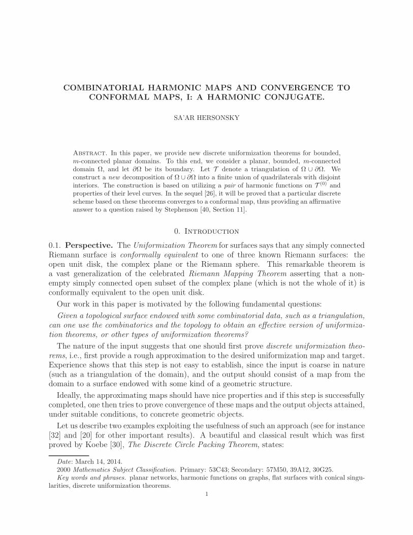
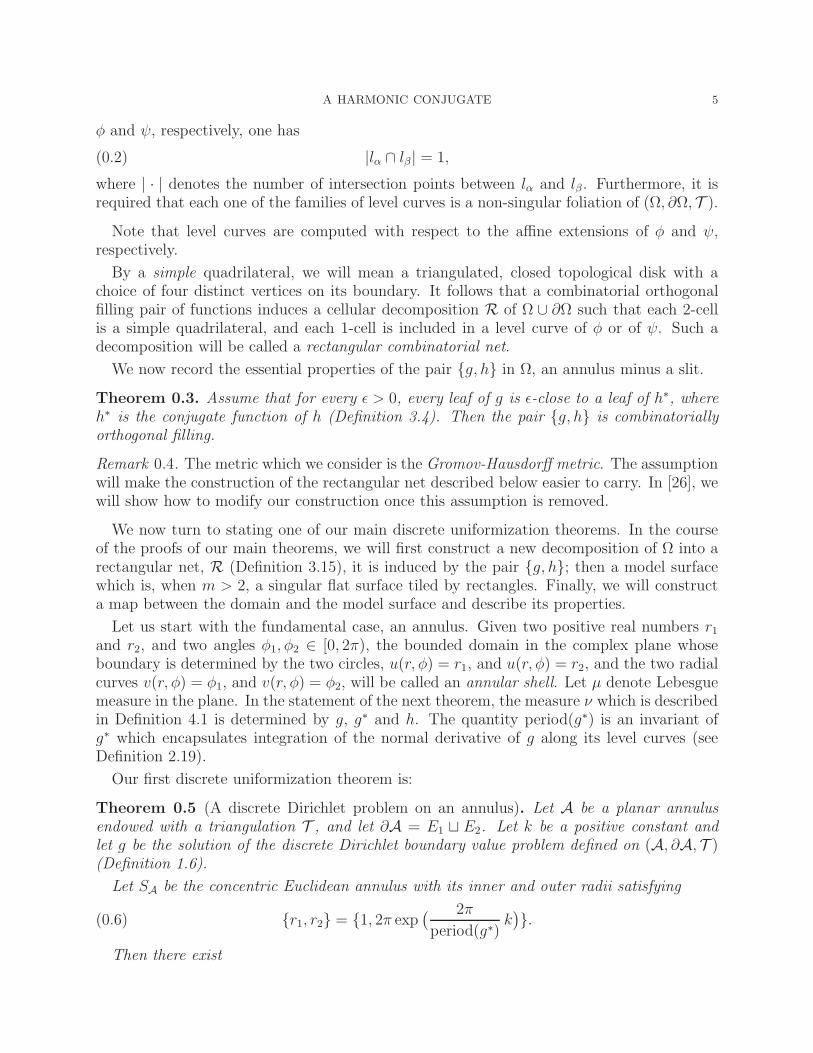
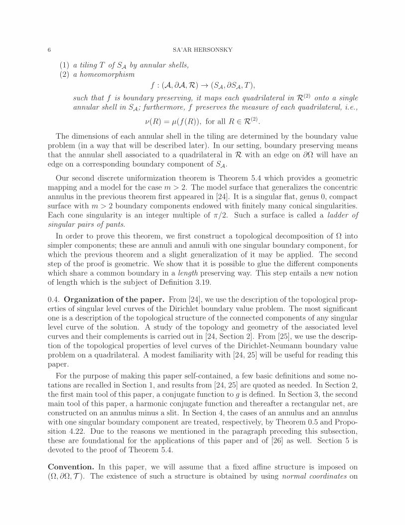
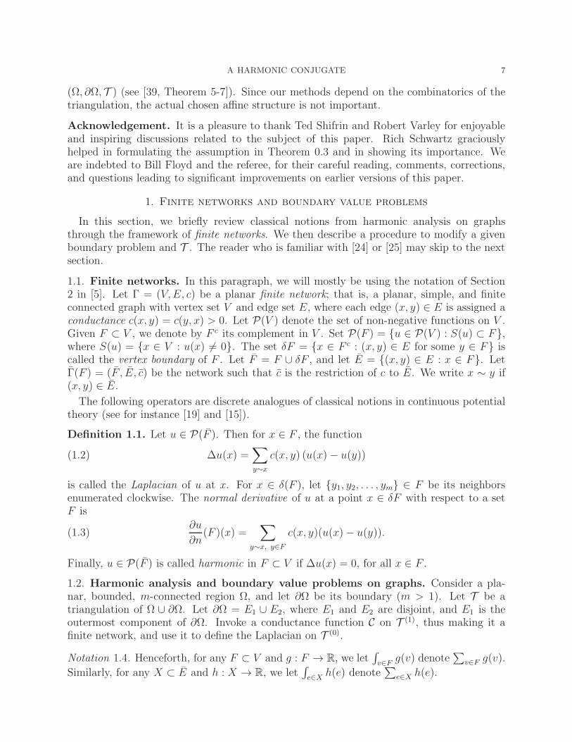
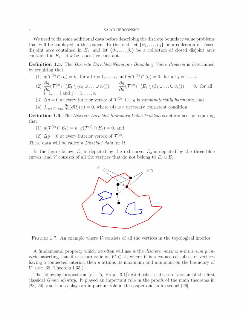
In the figure below, E1 is depicted by the red curve, E2 is depicted by the three bluecurves, and V consists of all the vertices that do not belong to E1 ∪ E2.

Eδ(V )

Figure 1.7. An example where V consists of all the vertices in the topological interior.

A fundamental property which we often will use is the discrete maximum-minimum prin-ciple, asserting that if u is harmonic on V ′ ⊂ V , where V is a connected subset of verticeshaving a connected interior, then u attains its maximum and minimum on the boundary ofV ′ (see [38, Theorem I.35]).

The following proposition (cf. [5, Prop. 3.1]) establishes a discrete version of the firstclassical Green identity. It played an important role in the proofs of the main theorems in[23, 24], and it also plays an important role in this paper and in its sequel [26].

A HARMONIC CONJUGATE 9

Proposition 1.8 (The first Green identity). Let F ⊂ V and u, v ∈ P(F ). Then we havethat

(1.9)

∫

(x,y)∈E

c(x, y)(u(x)− u(y))(v(x)− v(y)) =

∫

x∈F

∆u(x)v(x) +

∫

x∈δ(F )

∂u

∂n(F )(x)v(x).

1.3. Piecewise-linear modifications of a boundary value problem. We will often needto modify a given cellular decomposition, and thereafter to modify the initial boundary valueproblem. The need to do this is twofold. First assume, for example, that L is a fixed, simple,closed level curve of the initial boundary value problem. Since L ∩ T (1) is not (generically)a subset of T (0), Definition 3.19 may not be employed directly to provide a notion of lengthto L. Therefore, we will add vertices and edges according to the following procedure. Suchnew vertices will be called type I vertices.

Let O1,O2 be the two distinct connected components of the complement of L in Ω, with Lbeing the boundary of both (these properties follow by employing the Jordan curve theorem).We will call O1 an interior domain if all the vertices which belong to it have g-values that aresmaller than the g-value of L. The other domain will be called the exterior domain. Notethat by the maximum principle, one of O1,O2 must have all of its vertices with g-valuessmaller than the g-value of L.

Let e ∈ T (1), and assume that x = e ∩ L is a vertex of type I. Thus, two new edges (x, v)and (u, x) are created. We may assume that v ∈ O1 and u ∈ O2. Next, define conductanceconstants c(v, x) = c(x, v) and c(x, u) = c(u, x) by

(1.10) c(v, x) =c(v, u)(g(v)− g(u))

g(v)− g(x)and c(u, x) =

c(v, u)(g(u)− g(v))

g(u)− g(x).

By adding to T all such new vertices and edges, as well as the piecewise arcs of L deter-mined by the new vertices, we obtain two cellular decompositions, TO1 of O1 and TO2 of O2.Note that in general, new two cells that are quadrilaterals are introduced.

Two conductance functions, CO1 and CO2 , are now defined on the one-skeleton of these cel-lular decompositions, by modifying according to Equation (1.10) the conductance constantsthat were used in the Dirichlet data for g (i.e., changes are occurring only on new edges, andon L the conductance is defined to be identically zero). One then defines (see [24, Definition2.7]) a natural modification of the given boundary value problem, the solution of which iseasy to control by using the existence and uniqueness theorems in [5]. In particular, it isequal to the restriction of g to Oi, for i = 1, 2.

Another technical point which motivates the modification described above will manifestitself in Subsection 3.3. Proposition 1.8 will be frequently used in this paper, and it maynot be directly applied to a modified cellular decomposition, and the modified boundaryvalue problem defined on it. Formally, in order to apply Proposition 1.8 to a meaningfulboundary value problem, the modified graph of the network needs to have its vertex boundarycomponents separated enough in terms of the combinatorial distance. Whenever necessary,we will add new vertices along edges and change the conductance constants along new edgesin such a way that the solution of the modified boundary value problem will still be harmonicat each new vertex, and will preserve the values of the solution of the initial boundary value

10 SA’AR HERSONSKY

problem at the two vertices along the original edge. Such vertices will be called type IIvertices.

Formally, once such changes occur, a new Dirichlet boundary value problem is defined.The existence and uniqueness of the solution of a Dirichlet boundary value problem (see [5])allows us to abuse notation and keep denoting the new solution by g. We will also keepdenoting by T any new cellular decomposition obtained as described above.

2. constructing a conjugate function on an annulus with a slit

This section has two subsections. The first subsection contains the construction of theconjugate function g∗ to the solution of the initial Dirichlet boundary value problem definedon an annulus. The second subsection is devoted to the study of the level curve of theconjugate function. In particular, to the interaction between these and the level sets of g.

2.1. Constructing the conjugate function g∗. In this subsection, we will construct afunction, g∗, which is conjugate in a combinatorial sense to g (the solution of a Dirichletboundary value problem defined on an annulus). The conjugate function will be singlevalued on the annulus minus a chosen slit.

Keeping the notation of the previous section and the introduction, let (A, ∂Ω = E1∪E2, T )be an annulus endowed with a cellular decomposition in which each 2-cell is either a triangleor a quadrilateral. Let k be a positive constant, and let g be the solution of a Dirichletboundary value problem as described in Definition 1.6. Note that all the level curves of g arepiecewise, simple, closed curves separating E1 and E2 (see Lemma 2.8 in [24] for the analysisin this case and the case of higher connectivity) which foliate A.

Before providing the definition of the conjugate function, we need to make a choice of apiecewise linear path in A.

Definition 2.1. Let slit(A) denote a fixed, simple, combinatorial path in T (1) which joinsE1 to E2. Furthermore, we require that the restriction of the solution of the discrete Dirichletboundary value problem to it is monotone decreasing.

Remark 2.2. The existence of such a path is guaranteed by the discrete maximum principle.

Let

(2.3) L = L(v0), . . . , L(vk)

be the collection of level curves of g that contain all the vertices in T (0) arranged accordingto increasing values of g. It follows from Definition 1.6 that L(v0) = E2 and L(vk) = E1. Wealso add vertices of Type II so that any two level sets in L are at (combinatorial) distanceequal to two. This can be done in various ways, henceforth, we will assume that one of theseis chosen.

We wish to construct a single valued function on A. In order to do so, we will start with apreliminary case. To this end, let Qslit denote the quadrilateral obtained by cutting open Aalong slit(A) and having two copies of slit(A) attached, keeping the conductance constantsalong the split edges. Since an A orientation is well defined, we will denote one of the twocopies by ∂Qbase, and the other by ∂Qtop. In other words, from the point of view of A, pointson slit(A) may be endowed with two labels, recording whether they are the starting point of

A HARMONIC CONJUGATE 11

a level curve (with winding number equal to one) or its endpoint. We keep the values of gat the vertices unchanged. Thus, corresponding vertices in ∂Qbase and ∂Qtop have identicalg-values. By abuse of notation, we will keep denoting by T (0) the 0-skeleton of Qslit.

L(v)

A

E2

E1

v

slit(A)

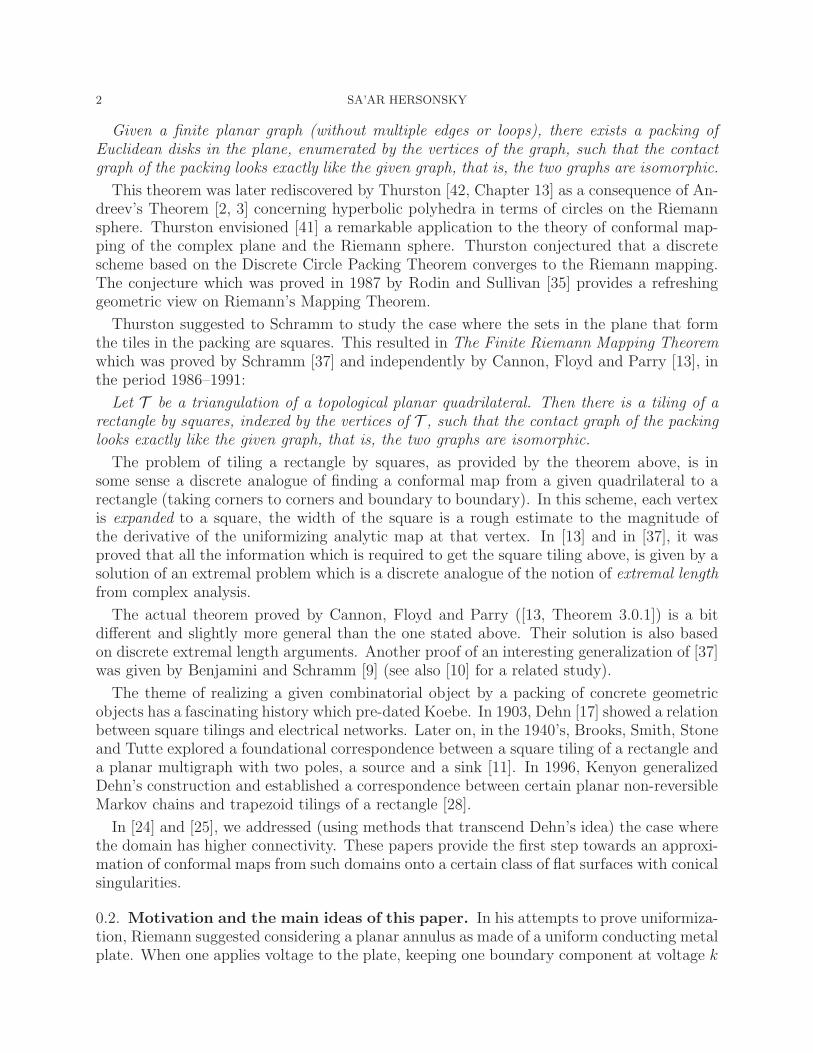
Qvπ(v)

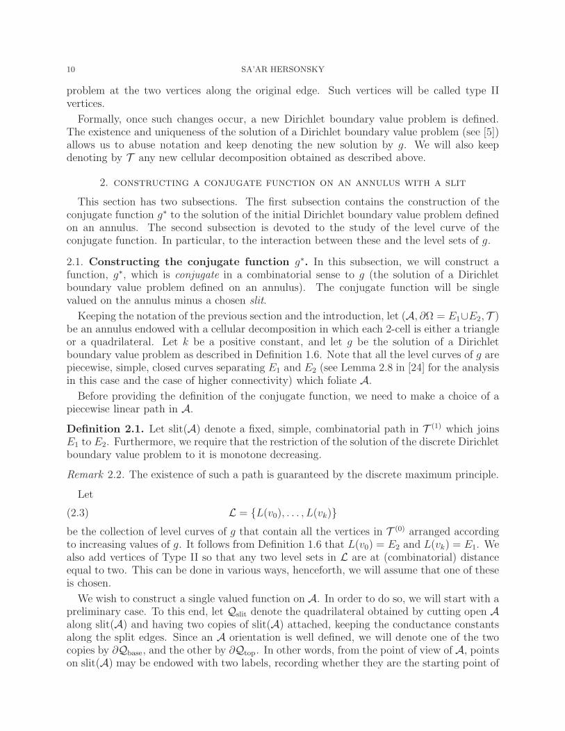
Figure 2.4. An example of a quadrilateral Qv.

For v ∈ A \ E2, which is in T (0) or a vertex of type I, let L(v) denote the unique levelcurve of g which contains v. Let Qv be the interior of the piecewise-linear quadrilateralwhose boundary is defined by ∂Qbase, ∂Qtop, L(v) and E2. For v ∈ E2, which is in T (0) or avertex of type I, Qv is defined to be (the interior of) Qslit.

Remark 2.5. Recall that a vertex of type I is introduced whenever the intersection betweenan edge and the level curve does not belong to T (0).

We now make

Definition 2.6 (The Conjugate function of g). Let v be a vertex in T (0) or a vertex of typeI. Let

(2.7) π(v) = L(v) ∩ ∂Qbase.

We define g∗(v), the conjugate function of g, as follows.

First case: Suppose that v 6∈ E2 ∪ ∂Qtop. Then

(2.8) g∗(v) =

∫ v

π(v)

∂g

∂n(Qv)(u),

where the integration is carried along (the vertices of) L(v) in the counter-clockwisedirection.

12 SA’AR HERSONSKY

Second case: Suppose that v ∈ E2 \ ∂Qtop. Then we define g∗(v) by

(2.9) g∗(v) =

∫ v

π(v)

−∂g

∂n(Qv)(u) =

∫ v

π(v)

∣

∣

∂g

∂n(Qv)(u)

∣

∣,

where the integration is carried along (the vertices of) E2 in the counter-clockwise direction.

On edges in ∂Qtop, we record the conductance constants induced byA. In order to define g∗

on ∂Qtop, we consider the vertices on ∂Qtop as vertices in A. For the single vertex ∂Qtop∩E2,the integration above is modified to include the contribution of its normal derivative fromits rightmost neighbor in ∂Qtop. For any other vertex in ∂Qtop, the integration above ismodified to include the contribution of its normal derivative from its leftmost neighbor in∂Qtop. Finally, for a point z ∈ Qslit which is not a vertex, g∗(z) is defined by extending g∗

affinely over edges and triangles, and bi-linearly over quadrilaterals.

Remark 2.10. The absolute value of the normal derivative of g at a vertex which appears inEquation (2.9), is due to the maximum principle. The continuity of g∗ from the right on E2

follows from similar arguments to those appearing in the proof of Proposition 2.12 below.

Remark 2.11. Henceforth, we will denote by Q(E1), and by Q(E2), the two boundary com-ponents of Qslit, which correspond to their counterparts E1, and E2, respectively, in A.

We now turn to studying topological properties of the level curves of g∗.

By definition, ∂Qbase is the level curve of g∗ which corresponds to g∗ = 0. We will provethat ∂Qtop is also a level curve of g∗. In other words, computing the value of g∗ at theendpoint of a level curve emanating from ∂Qbase is independent of the level curve chosen.The proof is an application of the first Green identity (see Proposition 1.8).

Proposition 2.12. The curve ∂Qtop is a level curve of g∗.

Proof. Let L1 and L2 be any two level curves of g which start at ∂Qbase and have theirendpoints x1, and x2, on ∂Qtop, respectively. Let A(L1,L2) denote the (interior of) the annuluswhose boundary components are L1, and L2, respectively. Without loss of generality, assumethat the g-value of L1 is bigger than the g-value of L2. We must show that

(2.13) g∗(x1) = g∗(x2).

We now add vertices of type I and II according to the procedure defined in Subsection 1.3,so that the first Green identity, Proposition 1.8, may be applied to a Dirichlet boundaryvalue problem on the network induced on A(L1,L2).

Let w ≡ 1 be the constant function defined in A(L1,L2). The assertion of Proposition 1.8,applied with the functions w and g on the induced network in A(L1,L2), yields

(2.14)

∫

x∈T (0)∩∂A(L1,L2)

∂g

∂n(A(L1,L2))(x) = 0.

Hence, it follows that

(2.15)

∫

x∈T (0)∩L2

∂g

∂n(A(L1,L2))(x) +

∫

y∈T (0)∩L1

∂g

∂n(A(L1,L2))(y) = 0.

A HARMONIC CONJUGATE 13

(Note that vertices of type I appear in both of the integrals, so one must apply Equation (1.10)and the discussion preceding it to justify this equality.) It follows from Definition 2.6 thatthe second term in the above equations is equal to g∗(x1). Furthermore, since g is harmonicin T (0) ∩A, and since L2 is a level curve of g, it follows that

(2.16)

∫

x∈T (0)∩L2

∂g

∂n(A(L1,L2))(x) +

∫

x∈T (0)∩L2

∂g

∂n(A(E2,L2))(x) = 0.

As above, it follows from Definition 2.6 that the second term in the above equations isequal to −g∗(x2). Therefore, Equations (2.15) and (2.16) imply that

(2.17) g∗(x1) = g∗(x2).

This ends the proof of the Proposition.

Remark 2.18. With easy modifications, the proof goes through when L2 = E2.

We now make

Definition 2.19. The period of g∗ is defined to be the g∗ value on ∂Qtop, that is,

(2.20) period(g∗) = g∗(∂Qtop ∩ T (0)) =

∫

u∈T (0)∩E1

∂g

∂n(A(E2,E1))(u).

Following similar arguments to these in the proof above, it is easy to check that period(g∗)is independent of the choice of the added vertices of type II. Also, note that period(g∗) isindependent of the choice of the level curve chosen or the slit chosen. Indeed, it follows fromProposition 2.12 that for a fixed slit the computation of the period is independent of thepoints chosen on the slit.

Assume now that a different slit is chosen, and let η be the conjugate function correspond-ing to the new slit. It readily follows that period(η) = period(g∗).

Indeed, start with any point x on any of the two slits, let lx, the (unique) level curveof g passing through x. The computation of both periods is done by summing the normalderivative of g along (the whole of) lx, hence, they are equal. In fact, their common value isthe integral of the normal derivative of g along E2 (unless E1 is chosen so an absolute valueneeds to be applied to the end result).

We now continue the study of the level curves of g∗. Note that by the maximum principle(applied to g), and its definition, g∗ is monotone strictly increasing along level curves of g.This property will now be used in the following

Proposition 2.21. Each level curve of g∗ has no endpoint in the interior of Qslit, is simple,and joins Q(E1) to Q(E2). Furthermore, any two level curves of g∗ are disjoint.

Proof. Suppose that a level curve of g∗ which starts at s ∈ Q(E2) has an endpoint ξ inT ∈ T (2), where T lies in the interior of A. Let [s, ξ] be the intersection of this level curvewith the interior of A. Let Lξ denote the level curve of g that passes through ξ. Since thelevel curves of g foliate A, there exists a level curve Lψ of g, which is as close as we wish toLξ, and such that its intersection with [s, ξ] is empty. Since g∗ is monotone increasing and

14 SA’AR HERSONSKY

continuous along Lψ, it assumes all values between 0 and period(g∗). Hence, it will assumethe value g∗(ξ). This shows that no level curve of g∗ can have an interior endpoint.

Assume that one of the level curves of g∗ is not simple. Let D be any domain which isbounded by it. Since the level curves of g foliate the annulus, one of these intersects theboundary of D in at least two points. The monotonicity of g∗ along the level curves of grenders this impossible.

Assume that there exists a level curve of g∗, L(g∗), which does not join Q(E1) to Q(E2).By construction, each level curve of g∗ does not have an endpoint inside A and its intersectionwith each 2-cell is a segment (or a point). Hence, both endpoints of L(g∗) must lie on Q(E1)or on Q(E2). Without loss of generality, assume that both endpoints are on Q(E1). Hence,there must be a level curve of g that intersects L(g∗) in at least two points. Reasoning in asimilar way to the paragraph above, this easily leads to a contradiction.

The fact that level curves of g∗ that correspond to the same value may not intersect eachother follows from similar arguments to those appearing in the first parts of the proof.

Of special importance is the interaction between the level curves of g∗ and the level curvesof g. The following proposition states that, from a topological point of view, the union ofthe two families of level curves resembles a planar coordinate system. This proposition isone topological prerequisite for the proof of Theorem 0.3, which will appear in the nextsubsection.

Proposition 2.22. The number of intersections between any level curve of g∗ and any levelcurve of g is equal to 1.

Proof. It readily follows from the proof of Proposition 2.21 that the number of intersectionsof any level curve of g with any level curve of g∗ is at most equal to one. Since both familiesof level curves foliate Qslit, this number is equal to one.

3. Constructing a harmonic conjugate and the proof of theorem 0.3

This section has three subsections. In the first, we define the harmonic conjugate functionh and study its immediate properties. In the second, we provide the proof of Theorem 0.3.In the third, we define the pair-flux metric and its induced length. These notions will beessential to the proof of Theorem 5.4 in which gluing two components of the complement ofa singular level curve of the solution takes place.

3.1. A harmonic conjugate function. We keep the notation of the previous section andmodify Definition 1.5 to the case of Qslit.

Definition 3.1. The harmonic conjugate function h is the solution of the discrete Dirichlet-Neumann boundary value problem defined by

(1) h(T (0) ∩ ∂Qtop) = period(g∗), and h(T (0) ∩ ∂Qbase) = 0,

(2)∂h

∂n(T (0) ∩Q(E1)) =

∂h

∂n(T (0) ∩Q(E2)) = 0 (other than at the four corners of Qslit),

(3) ∆h = 0 at every (interior) vertex of T (0) ∩Qslit, and

A HARMONIC CONJUGATE 15

(4)∫

x∈T (0)∩∂Qslit

∂h∂n(∂Ω)(x) = 0, where (4) is a necessary consistent condition.

Consider now

(3.2) M = M(v0), . . . ,M(vp),

the collection of level curves of h, that contain all the vertices in T (0) arranged according toincreasing values of h. It follows from the definition of h that M(v0) = Qbase and M(vp) =Qtop.

We will now define the conjugate function of h, which will be denoted by h∗, to thecase of the quadrilateral Qslit; it is a straightforward modification of the definition of g∗

(Definition 2.6).

Indeed, one recalls that by [25, Proposition 2.1] the level curves of h are disjoint, piecewise-linear simple curves that foliate Qslit and join Q(E1) to Q(E2).

For v ∈ Qslit\Qbase, which is in T (0) or a vertex of type I, letM(v) denote the unique levelcurve of h which contains v. Let Pv be the piecewise-linear quadrilateral whose boundary isdefined by Q(E1),M(v), Q(E2) and Qbase. For v ∈ Qbase, recall that Qbase = M(v0) is theunique level curve of h which contains v. Let Pv be equal to Qslit.

Remark 3.3. Note that a vertex of type I is introduced whenever the intersection betweenan edge and the level curve does not belong to T (0).

Definition 3.4 (The conjugate function of h). Let v be a vertex in T (0) ∩ Qslit or a vertexof type I. Let

(3.5) π(v) =M(v) ∩Q(E1).

We define h∗(v), the conjugate function of h, as follows.

First case: Suppose that v 6∈ Qbase. Then

(3.6) h∗(v) =

∫ v

π(v)

∂h

∂n(Pv)(u),

where the integration is carried along (the vertices of) M(v) (from π(v) to v).

Second case: Suppose that v ∈ Qbase. Then we define h∗(v) by

(3.7) h∗(v) =

∫ v

π(v)

∣

∣

∂h

∂n(Pv)(u)

∣

∣,

where the integration is carried along (the vertices of) Qbase (from π(v) to v).

For a point z ∈ Qslit, which is not a vertex as above, h∗(z) is defined by extending h∗

affinely over edges and triangles, and bi-linearly over quadrilaterals.

We now turn to studying a few topological properties of the level curves of h∗ and theirinteraction with the level curves of h. The statements and the proofs are immediate general-izations of their counterparts in Section 2, and therefore we omit the proofs. The interactionbetween the level curves of g and those of h is subtle and will be treated in the next subsec-tion.

16 SA’AR HERSONSKY

By definition, Q(E1) is the level curve of h∗ which corresponds to h∗ = 0. It will followthat Q(E2) is also a level curve of h∗. In other words, computing the value of h∗ at theendpoint of a level curve emanating from Q(E1) is independent of the level curve chosen.We recall this property in

Proposition 3.8. The curve Q(E2) is a level curve of h∗ in Qslit.

The proof is an application of the first Green identity (see Proposition 1.8) and is a directgeneralization of the method of proof of Proposition 2.12 applied to Pv where v ∈ E2.Although not used in this paper, as a consequence of this proposition, we can now make

Definition 3.9. The width of h∗ is defined to be the h∗ value on Q(E2), that is,

(3.10) width(h∗) = h∗(Q(E2) ∩ T (0)).

Note that by the maximum principle (applied to h), and by its definition, h∗ is monotonestrictly increasing along level curves of h. This property is used in proving the followingproposition in exactly the same way that the analogous property for the pair g, g∗ wasused in the proof of Proposition 2.21.

Proposition 3.11. Each level curve of h∗ has no endpoint in the interior of Qslit, is simple,and joins Qbase to Qtop. Furthermore, any two level curves of h∗ are disjoint.

Of special importance is the interaction between the level curves of h∗ and the levelcurves of h. The following proposition will show that, from a topological point of view, theunion of the two families of level curves of h, h∗ resembles a planar coordinate system.This proposition is another topological prerequisite for the proof of Theorem 0.3, which willappear in the next subsection.

Proposition 3.12. The number of intersections between any level curve of h∗ and any levelcurve of h is equal to 1.

The proof is an immediate modification of the proof of Propostion 2.22 to the case of thepair h, h∗.

3.1.1. Viewing h from a PDE perspective. The term “harmonic conjugate” associatedwith h is motivated by the first three properties used to define h (Definition 3.1). Hence, hsatisfies the combinatorial analogues of the analytical properties of the polar angle functionv(r, φ) = φ in the complex plane, which is known to be, when it is single-value defined, theharmonic conjugate function of v(r, φ) = r.

3.1.2. Related work. Our definition of the harmonic conjugate function is motivated by thefact that, in the smooth category, a conformal map is determined by its real and imaginaryparts, which are known to be harmonic conjugates. The search for discrete approximation ofconformal maps has a long and rich history. We refer to [33] and [14, Section 2] as excellentrecent accounts.

We should also mention that a search for a combinatorial Hodge star operator has recentlygained much attention and is closely related to the construction of a harmonic conjugatefunction. We refer the reader to [27] and to [34] for further details and examples for suchcombinatorial operators.

A HARMONIC CONJUGATE 17

3.2. The proof of Theorem 0.3. Each vertex in T (0) (which is now a modification of theoriginal one by adding all the vertices of type I in Qslit) belongs to one and only one of thelevel curves of h. Let

(3.13) M = M(v0), . . . ,M(vp)

be defined according to Equation (3.2); this is the set of level curves of h, arranged accordingto increasing values of h, which contain all of the vertices mentioned above. Recall thatM(v0) = Qbase and M(vp) = Qtop. Let

(3.14) L = L(v0), . . . , L(vk)

be defined according to Equation (2.3); this is the set of level curves of g, arranged accordingto increasing values of g, which contain all of the vertices mentioned above. Recall thatQ(E2) ⊂ L(v0) and Q(E1) ⊂ L(vk).

We will now study the following decomposition of Ω ∪ ∂Ω.

Definition 3.15. Let R be the decomposition of Ω∪ ∂Ω induced by the intersection of thesets M,L.

Since each one of the sets of level curves of g, h, respectively, is clearly dense in Ω ∪ ∂Ω,in order to prove Theorem 0.3 it suffices to establish

Proposition 3.16 (A rectangular net). The number of intersections between any level curveof g and any level curve of h is equal to 1.

Once this proof is furnished, it will follow that the each 2-cell in R is a quadrilateral, whereeach pair of opposite boundaries is contained in successive level sets of h or in successivelevel sets of g. Note that a vertex is formed in R(0), whenever a level set of g and a level setof h intersect.

Proof of Proposition 3.16. We argue by contradiction. It follows from [24, Lemma 2.8] and[25, Proposition 2.1] that the level curves of g as well as the level curves of h foliate Qslit;hence, the number of intersections between a level curve of g and a level curve of h is atleast one.

By Proposition 3.12, the number of intersections between any level curve of h and anylevel curve of h∗ is exactly one. Hence, the proof of the Proposition will readily follow fromthe following lemma, where the level curves of g∗ and h∗ play an important role.

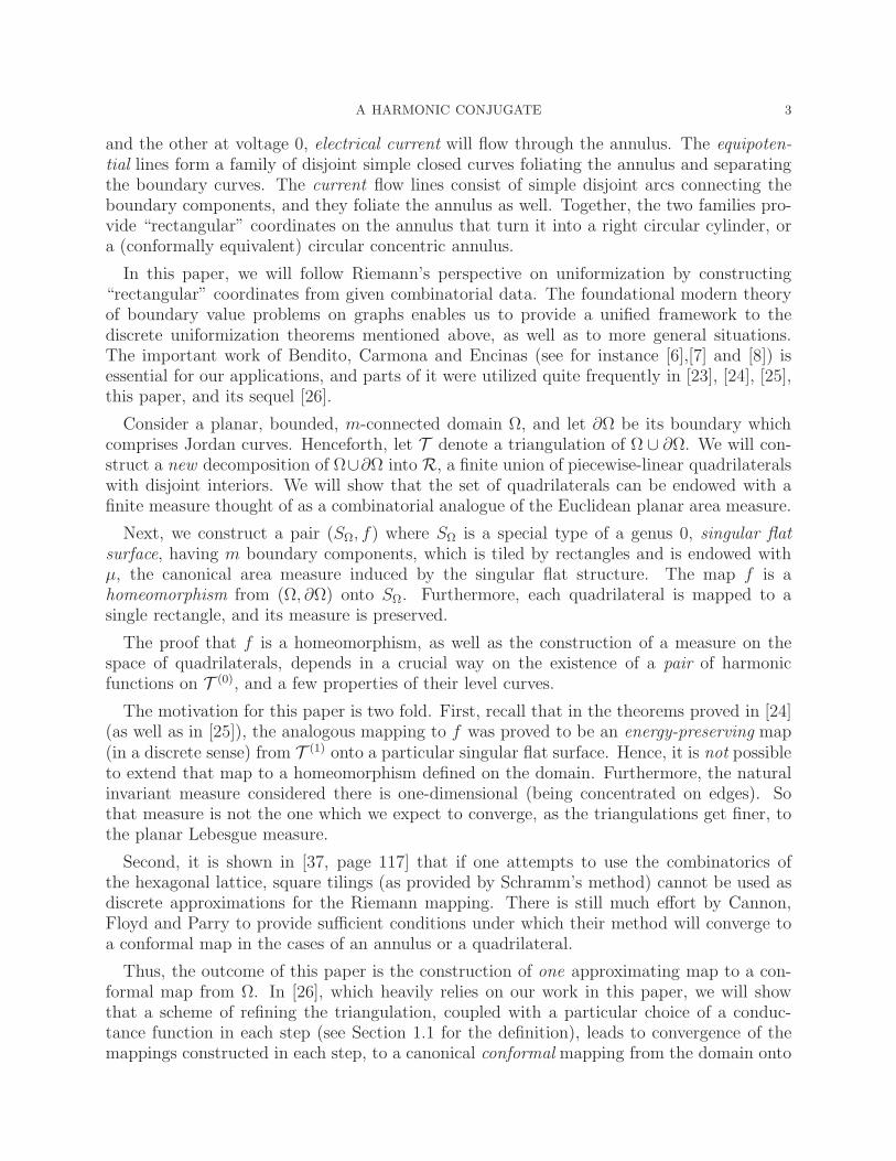
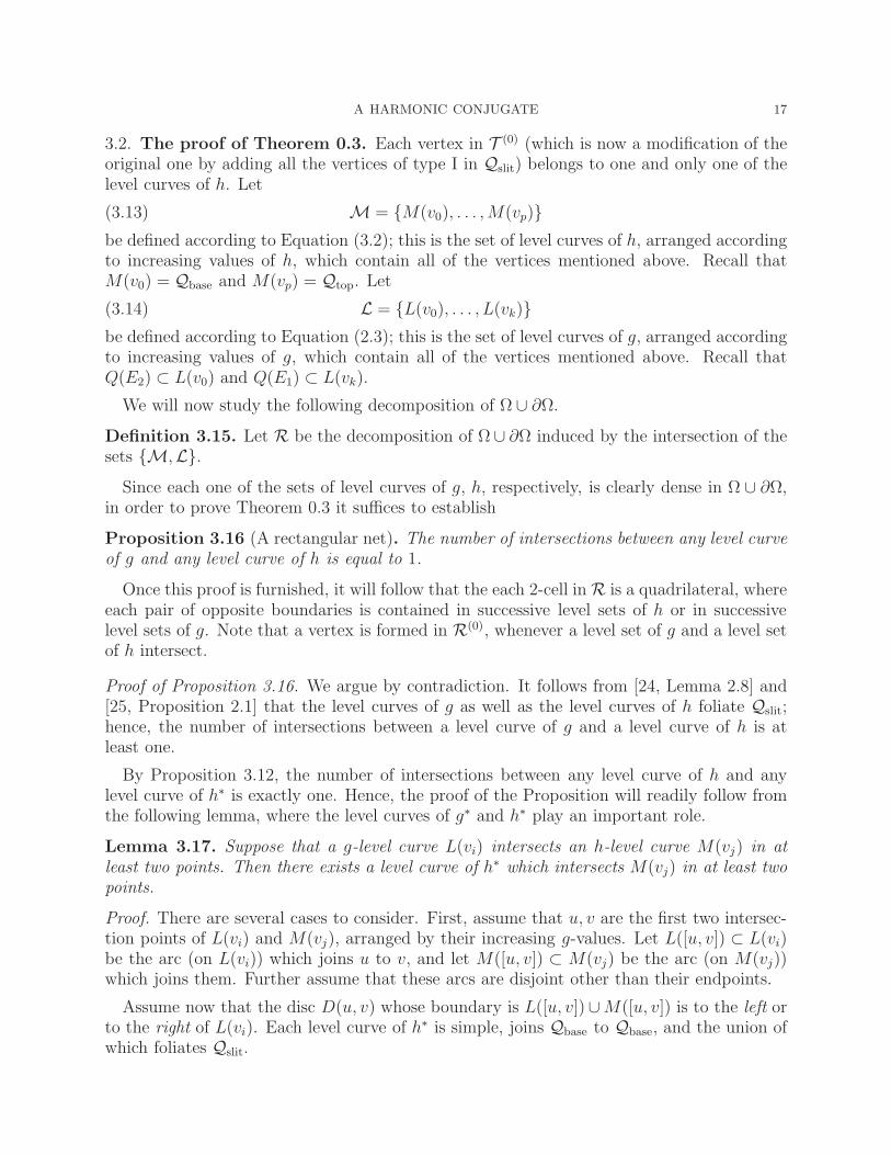
Lemma 3.17. Suppose that a g-level curve L(vi) intersects an h-level curve M(vj) in atleast two points. Then there exists a level curve of h∗ which intersects M(vj) in at least twopoints.

Proof. There are several cases to consider. First, assume that u, v are the first two intersec-tion points of L(vi) and M(vj), arranged by their increasing g-values. Let L([u, v]) ⊂ L(vi)be the arc (on L(vi)) which joins u to v, and let M([u, v]) ⊂ M(vj) be the arc (on M(vj))which joins them. Further assume that these arcs are disjoint other than their endpoints.

Assume now that the disc D(u, v) whose boundary is L([u, v])∪M([u, v]) is to the left orto the right of L(vi). Each level curve of h∗ is simple, joins Qbase to Qbase, and the union ofwhich foliates Qslit.

18 SA’AR HERSONSKY

L(vi)

Q(E1)

Qtop

L∗h(vi)

u

D(u, v)

v

M(vj)

Qbase

Q(E2)

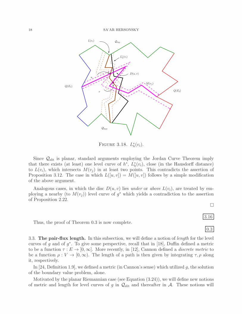
Figure 3.18. L∗h(vi).

Since Qslit is planar, standard arguments employing the Jordan Curve Theorem implythat there exists (at least) one level curve of h∗, L∗

h(vi), close (in the Hausdorff distance)to L(vi), which intersects M(vj) in at least two points. This contradicts the assertion ofProposition 3.12. The case in which L([u, v]) = M([u, v]) follows by a simple modificationof the above argument.

Analogous cases, in which the disc D(u, v) lies under or above L(vi), are treated by em-ploying a nearby (to M(vj)) level curve of g∗ which yields a contradiction to the assertionof Proposition 2.22.

3.16Thus, the proof of Theorem 0.3 is now complete.

0.3

3.3. The pair-flux length. In this subsection, we will define a notion of length for the levelcurves of g and of g∗. To give some perspective, recall that in [18], Duffin defined a metricto be a function τ : E → [0,∞]. More recently, in [12], Cannon defined a discrete metric tobe a function ρ : V → [0,∞). The length of a path is then given by integrating τ, ρ alongit, respectively.

In [24, Definition 1.9], we defined a metric (in Cannon’s sense) which utilized g, the solutionof the boundary value problem, alone.

Motivated by the planar Riemannian case (see Equation (3.24)), we will define new notionsof metric and length for level curves of g in Qslit and thereafter in A. These notions will

A HARMONIC CONJUGATE 19

incorporate both g and g∗. (We will of course consider these notions for level curves thatare given in their minimal form.)

Definition 3.19. With the notation of the previous sections, we define the following:

(1) For e = [e−, e+], let ψ(e) = e− be the map which associates to an edge its initialvertex. The pair-flux weight of e is defined by

(3.20)

ρ(e) =2π

period(g∗)exp

( 2π

period(g∗)g(ψ(e))

)

|dh(e)| =2π

period(g∗)exp

( 2π

period(g∗)g(e−))

)

|dh(e)|,

where dh(e) = h(e+)− h(e−).

(2) Let L be any path in R; then its length with respect to the pair-flux weight is givenby integrating ρ along it,

(3.21) Length(L) =

∫

e∈L

ρ(e).

In the applications of this paper, we will use the pair-flux weight to provide a notion oflength to level curves of g. Thus, by the assertion of Proposition 2.12, we may now deduce

Corollary 3.22. Let L(v) be a closed level curve of g (oriented counter-clockwise), and let0 ≤ m = g(L(v)) ≤ k; then we have

(3.23) Length(L(v)) = 2π exp( 2π

period(g∗)m)

.

The definition of the pair-flux length is one of the new advances of this paper. Whereasin [24, 25, 26] other notions of lengths utilizing only the solution g were introduced, thepair-flux length incorporates the pair g, h. This appealing feature is motivated by the casein the smooth category, i.e., for z = r exp (iθ) in the complex plane, we have

(3.24) dz = ir exp (iθ)dθ + exp (iθ)dr.

We will now provide a notion of length to the level curves of h in Qslit, and thereafter inA. Keeping the analogy with the planar Riemannian case, the restriction of the Euclideanlength element to level curves of the function v(r, φ) = φ0, has the form

(3.25) |dz| = dr.

Definition 3.26. Let L(h) = (v0, . . . , vk) be a level curve of h with v0 ∈ E2 and vk ∈ E1,then its length is given by

(3.27) Length(L(h)) = exp(g(vk))− exp(g(v0)) = exp(k)− 1.

Remark 3.28. It is a consequence of Proposition 3.8 that any two level curves of h have thesame length.

20 SA’AR HERSONSKY

4. The cases of an annulus and an annulus with one singular boundary

component

4.1. The case of an annulus. In this subsection, we study the important case of an an-nulus. It is the first case, in terms of the connectivity of the domain Ω, of the one describedin Definition 1.6 (Subsection 1.2). Let R be the rectangular net associated with the combi-natorial orthogonal filling pair g, h which was constructed in the proof of Theorem 0.3.

We use the term measure on the space of quadrilaterals in R(2) to denote a non-negativeset function defined on R(2). An example of such, which will be used in Theorem 0.5, isprovided in

Definition 4.1. For any R ∈ R(2), let Rtop, Rbase be the pair of its opposite boundariesthat are contained in successive level sets of g; we will denote them by the top and baseboundaries of R, respectively (where the top boundary corresponds to a larger value of g).

Let t ∈ R(0)top and b ∈ R

(0)base be any two vertices. Then we let

(4.2) ν(R) =1

2

(

exp2(2π

period(g∗)g(t))− exp2(

2π

period(g∗)g(b))

)2π dh(Rbase)

period(g∗).

Remark 4.3. By the construction of R, all the vertices in Rtop (Rbase) have the same g valuesand dh(Rbase) = dh(Rtop).

We now turn to the

Proof of Theorem 0.5. Recall (see the discussion preceding the proof of Theorem 3.16)that the vertices in R(0) are comprised of all the intersections of the level curves of g (thefamily L) and the level curves of h (the family M). Thus, the vertex (i, j) will denotethe unique vertex determined by the intersection of L(vi) and M(vj); the existence anduniqueness of this intersection are consequences of Theorem 3.16.

The harmonic conjugate function h is single-valued onQslit, and multi-valued with a periodwhich is equal to period(g∗), when extended to A. This means that

(4.4) h(z1) = h(z0) + period(g∗),

whenever z1 ∈ L(z0) is obtained from z0 ∈ slit(A) by traveling one full cycle along the g-level curve L(z0). Hence, the function

(4.5)2π

period(g∗)

(

g(v) + ih(v)), v ∈ A ∩R(0)

has period 2πi when defined on A. Therefore,

(4.6) exp( 2π

period(g∗)

(

g(v) + ih(v)))

, v ∈ A ∩R(0)

is single-valued on A.

We now turn to the construction of the tiling T .

A HARMONIC CONJUGATE 21

The tiling T of SA is determined by all the intersections of the family of concentric circles,C, defined by

(4.7) ri = exp( 2π

period(g∗)g(vi)

)

, for i = 0, . . . , k,

with the family of radial lines Γ, defined by

(4.8) φj =2π

period(g∗)h(vj), for j = 0, . . . , p,

where each annular shell in the tiling is uniquely defined by four vertices that lie on twoconsecutive members of the families above.

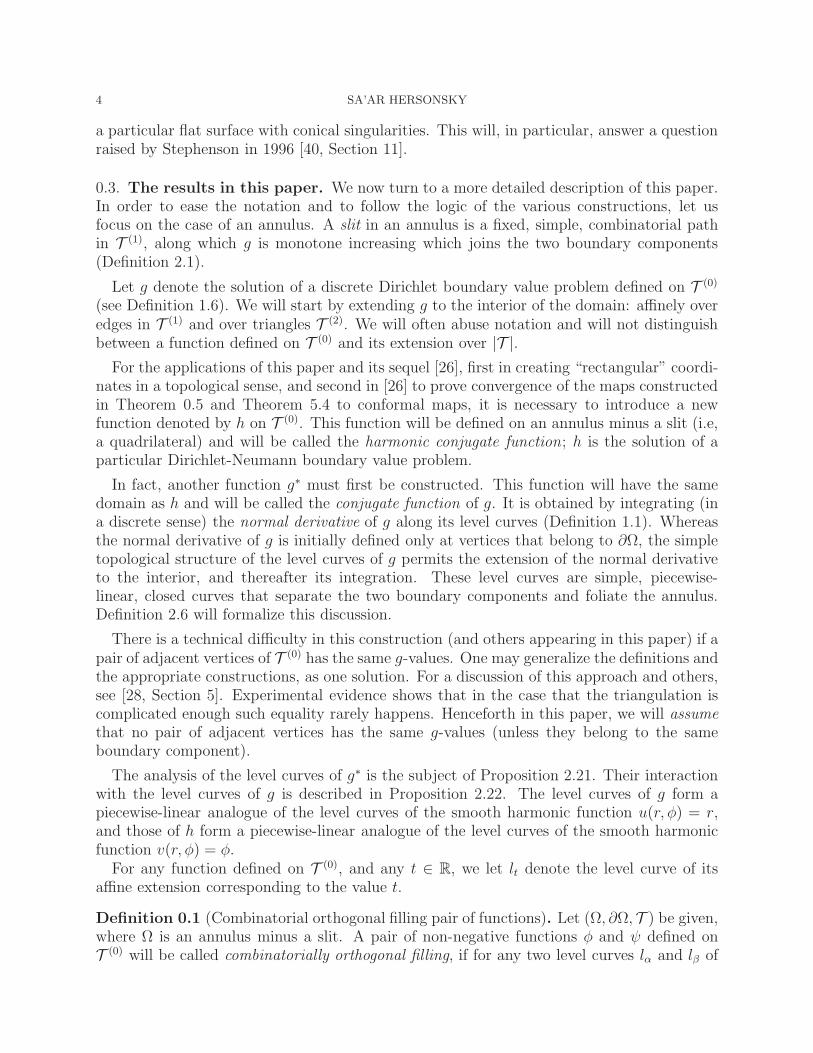
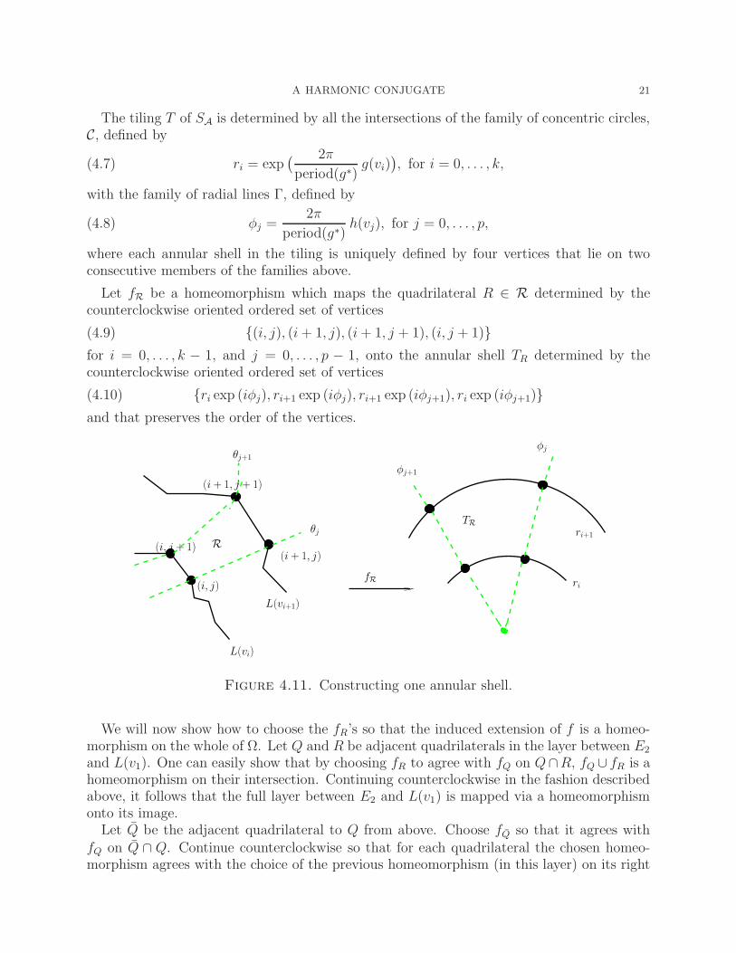
Let fR be a homeomorphism which maps the quadrilateral R ∈ R determined by thecounterclockwise oriented ordered set of vertices

(4.9) (i, j), (i+ 1, j), (i+ 1, j + 1), (i, j + 1)

for i = 0, . . . , k − 1, and j = 0, . . . , p − 1, onto the annular shell TR determined by thecounterclockwise oriented ordered set of vertices

(4.10) ri exp (iφj), ri+1 exp (iφj), ri+1 exp (iφj+1), ri exp (iφj+1)

and that preserves the order of the vertices.

fR

(i + 1, j + 1)

(i + 1, j)

(i, j)

(i, j + 1)

TR

R

L(vi)

L(vi+1)

φj

φj+1

θj+1

θj ri+1

ri

Figure 4.11. Constructing one annular shell.

We will now show how to choose the fR’s so that the induced extension of f is a homeo-morphism on the whole of Ω. Let Q and R be adjacent quadrilaterals in the layer between E2

and L(v1). One can easily show that by choosing fR to agree with fQ on Q∩R, fQ ∪ fR is ahomeomorphism on their intersection. Continuing counterclockwise in the fashion describedabove, it follows that the full layer between E2 and L(v1) is mapped via a homeomorphismonto its image.

Let Q be the adjacent quadrilateral to Q from above. Choose fQ so that it agrees withfQ on Q ∩ Q. Continue counterclockwise so that for each quadrilateral the chosen homeo-morphism agrees with the choice of the previous homeomorphism (in this layer) on its right

22 SA’AR HERSONSKY

edge, and also agrees on its base, with the choice of the homeomorphism for the quadrilateralunder it (on its top).

For the last quadrilateral in this layer, a homeomorphism can be chosen to agree with thefirst chosen homeomorphism (in this layer) on its left side, with the homeomorphism chosenbefore it on its right side, and agrees (on its base) with the homeomorphism chosen for thequadrilateral lying under it. We continue this process, a layer by layer, until the domain isexhausted.

Let

(4.12) f =⋃

R∈R(2)

fR.

It is clear from (4.9) and (4.10) that f maps any edge in R(1)∩∂Ω homeomorphically ontoan arc in ∂SA. Therefore, f is indeed boundary preserving.

It remains to prove that the map f = ∪RfR which is assembled from the individual maps asdefined above is a homeomorphism onto SA. To this end, first observe that by the maximumprinciple, the map f is into SA.

By the definitions of ν, µ and TR, we have for all R ∈ R(2) that

(4.13) ν(R) = µ(TR).

It is clear from the construction of R that any two quadrilaterals in R(2) have disjointinteriors and that their intersection is either a single vertex or a common edge. Also recallthat by definition each quadrilateral has its top and bottom edges situated on two successivelevel curves in L, and its right and left edges situated on two successive level curves in M.

Since the union of the quadrilaterals in R(2) tile A, the total ν-measure of their union,which we define to be ν(A), satisfies the following

(4.14) ν(A) ≡ ν(∪R∈R(2)R) =∑

R∈R(2)

ν(R).

Starting from the quadrilaterals that lie between L(v0) and L(v1), we sum the ν-measureof all the quadrilaterals in the layer defined in between successive level curves of g, until wereach L(vk). By employing Definition 4.1 an easy computation shows that

(4.15) ν(A) = π(

exp2( 2π

period(g∗)k)

− 1)

.

By the construction of the annular shells and the definition of the map f , each quadrilateralR is mapped onto a unique annular shell TR. No two different quadrilaterals are mappedonto the same annular shell, and the collection of their images tiles a subset of SA.

Hence, by applying the above paragraph, (4.14), (4.13), (4.15) and the definition of SA,we obtain that

(4.16) ν(A) =∑

R∈R(2)

µ(TR) = µ(⋃

R∈R(2)

TR) = µ(SA).

A HARMONIC CONJUGATE 23

Hence, there are no gaps nor overlaps in the tiling of SA and therefore f is onto.

This concludes the proof of the theorem.

Remark 4.17. The proof shows that each curve in set L is mapped homemorphically onto a(unique) level curve in the family u(r, φ) = ri, and that each curve in the set M is mappedhomeomorphically onto a (unique) level curve in the family v(r, φ) = φj . Also, the discussionfollowing Definiton 2.19 guarantees that the dimensions of SA are independent of the choiceof the slit chosen.

4.1.1. Relation of Theorem 0.5 to works by Schramm and Cannon-Floyd-Parry.

It is imperative to relate this theorem to Theorem 1.3 in [37], and Theorem 3.0.1 in [13].While Schramm, and Cannon, Floyd, and Parry used discrete extremal lengths argumentsin their proofs, their arguments as well as their results are different. Schramm’s proof seemsto work for a quadrilateral but not directly for an annulus. The methods of Cannon, Floydand Parry work for both a quadrilateral and an annulus. Furthermore, Schramm’s inputis a triangulation with a contact graph that will (more or less) be preserved. The inputfor Cannon, Floyd and Parry is more flexible. They consider a covering of a topologicalquadrilateral (annulus) by topological disks. We refer the reader to the papers above fordetails. Upon applying a Dirichlet-Neumann boundary value problem, our methods of theproof of Theorem 0.5 may be adapted to work for the quadrilateral case as well.

While our proof of Theorem 0.5 does not use the machinery of extremal length arguments,it is worth recalling that in the smooth category there are celebrated connections betweenboundary value problems and extremal length (see for instance [1, Theorem 4.5]).

The common theme of our methods and those of Cannon, Floyd and Parry in [13] isthe construction of a new coordinate system on a topological annulus. As stated in theintroduction, this powerful idea goes back to Riemann.

4.2. The case of an annulus with one singular boundary component. In this subsec-tion, we will generalize Theorem 0.5 by providing a geometric model for an annulus with onesingular boundary component. The singular boundary component is of a special type. It isdetermined by the topological structure of a singular level curve of the solution of a Dirichletboundary value problem imposed on a planar embedded m-connected domain, where m > 1.

We start with two definitions; the first one appeared in [24, page 9].

Definition 4.18. A generalized bouquet of circles will denote a union of bouquets ofpiecewise-linear circles where the intersection of any two circles is at most a vertex. More-over, all such tangencies are required to be exterior, i.e., no circle is contained in the interiorof the bounded component of another.

Recall that Theorem 2.15, which was proved in [24], asserts the following.

Theorem 4.19 (The topology of a level curve). Let L be a level curve for g. Then eachconnected component of L is a generalized bouquet of circles.

24 SA’AR HERSONSKY

It is convenient to present the singular boundary component as a quotient space. In thefollowing definition, a circle will mean either a round circle or a piecewise linear circle.

We are now ready to make

Definition 4.20. An embedded planar circle with finitely many distinguished points on itwill be called a labeled circle. If in addition, equivalence relations among these points aregiven, so that the quotient of the labeled circle is a generalized bouquet of circles, then wecall the quotient a labeled bouquet, and the labeled circle will be called good.

Remark 4.21. Note that if a labeled round bouquet, i.e., one which consists of only roundcircles, has more than two round circles tangent at one point, it will no longer embed in R

2.

We will now define the object of study in this subsection. By a generalized singular annulus,Asing, we will mean a subset of the plane, whose interior is homeomorphic to the interior of

an annulus, and whose boundary has two components: one of which is homeomorphic to S1

and the other is a generalized bouquet of circles. The subscript denotes the set of tangencypoints in the generalized bouquet of circles. Let us also assume that a cellular decompositionT of (Asing, ∂Asing) is provided, where each 2-cell is either a triangle or a quadrilateral.

Topologically, Asing may be presented as the quotient of a planar annulus A, where

∂A = E1 ∪ E2, and E2 is a good labeled circle (see Definition 4.20). Henceforth, we will

let π denote the quotient map. We will let E2 denote the singular boundary component of∂Asing.

Note that the cellular decomposition T can be lifted to a cellular decomposition T of(A, ∂A), where each 1-cell, 2-cell in T , respectively, is the unique pre-image, under π−1, ofa unique 1-cell, 2-cell in T , respectively. The difference between the two cellular decompo-sitions manifests in the addition (in comparision to E2) of vertices in E2. Specifically, foreach vertex v in the singular part of ∂Asing, there are m(v) vertices in E2, where m(v) isthe number of circles that are tangent at v.

We will now apply Theorem 0.3 and Theorem 0.5 to (A, ∂A, T ). In the following proposi-tion, recall that the existence of R is provided by Theorem 0.3, and that h is the conjugateharmonic function to g, the solution of the imposed discrete Dirichlet boundary value prob-lem on (A, ∂A, T ) (see Definition 1.6).

With the above notation and setting in place, and with L denoting the set of level curvesof g as in Equation (2.3), we may now state the main proposition of this subsection.

Proposition 4.22 (An annulus with a singular boundary). Let (Asing, ∂Asing = E1∪E2) bea generalized singular annulus endowed with a cellular decomposition T . Let k be a positiveconstant, and let g be the solution of the discrete Dirichlet boundary value problem definedon (A, ∂A, T ).

Let SA be the concentric Euclidean annulus with its inner and outer radii satisfying

(4.23) r1, r2 = 1, 2π Length(L(vk)) = 1, 2π exp( 2π

period(g∗)k)

.

Then there exist

(1) a tiling T of SA by annular shells,

A HARMONIC CONJUGATE 25

(2) a set denoted by sing(SA) consisting of finitely many points which is contained in theinner boundary of SA,

(3) a homeomorphism

f : (A, ∂A \ π−1(sing(A)),R) → (SA, ∂SA \ sing(SA), T )

such that f maps the interior of each quadrilateral in R(2) onto the interior of asingle annular shell in SA, f preserves the measure of each quadrilateral, i.e.,

ν(R) = µ(f(R)), for all R ∈ R(2),

and f is boundary preserving.

Proof. The proof is a straightforward modification of the non-singular boundary case. Let Rbe the rectangular net constructed in Theorem 0.3. Let h be the conjugate harmonic functionconstructed on (A, ∂A, T ), let f be the homeomorphism constructed in Theorem 0.5, andlet T be the tiling of SA provided by Theorem 0.5.

For each ti ∈ sing(A) ⊂ E2, i = 1, . . . p, there are precisely m(ti) vertices on E2 in theequivalence class corresponding to ti. Let

(4.24) V(ti) = L(h)ti,1 , . . . , L(h)ti,m(ti), i = 1, . . . p

be the level curves of h that have one of their endpoints at one of these vertices. With thisnotation, and since the level curves of h are “parallel”, it follows that

(4.25) Vsing(A) =

p⋃

i=1

V(ti)

comprises of all the level curves of h that have an endpoint in the pre-image of sing(A).

Set

(4.26) sing(SA) = f(E2)⋂

f(

p⋃

i=1

V(ti)),

then sing(SA) is the image under f of all the vertices in the pre-image of sing(A). Further-more, recall that f(Vsing(SA)) is a set of radial arcs in SA.

To finish proving the statement in (3), note that any quadrilateral in R(2) whose verticesare disjoint from sing(SA) is mapped homemorphically onto a shell in SA. Since by construc-tion the image of π−1(sing(A)) is precisely sing(SA), it follows that f will map the interior ofeach one of the rest of the quadrilaterals homemorphically onto the appropriate shell, withpunctures at the corresponding vertices. This ends the proof of the proposition.

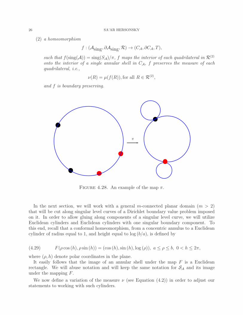
A geometric model to (Asing, ∂Asing, T ) is now easy to provide since the first part of

(3) in the proposition above allows us to label the vertices in sing(SA) isomorphically to thelabeling of the vertices in sing(A). We will keep denoting by π the quotient map which isthereafter induced on SA. Such a quotient annulus will be called a generalized Euclideanannulus and will be denoted by CA. The proof of the following corollary is straightforward.

Corollary 4.27. With the assumptions of Proposition 4.22, and with CA = SA/π, thereexist

(1) a tiling T of CA by annular shells, and

26 SA’AR HERSONSKY

(2) a homeomorphism

f : (Asing, ∂Asing,R) → (CA, ∂CA, T ),

such that f(sing(A)) = sing(SA)/π, f maps the interior of each quadrilateral in R(2)

onto the interior of a single annular shell in CA, f preserves the measure of eachquadrilateral, i.e.,

ν(R) = µ(f(R)), for all R ∈ R(2),

and f is boundary preserving.

π

Figure 4.28. An example of the map π.

In the next section, we will work with a general m-connected planar domain (m > 2)that will be cut along singular level curves of a Dirichlet boundary value problem imposedon it. In order to allow gluing along components of a singular level curve, we will utilizeEuclidean cylinders and Euclidean cylinders with one singular boundary component. Tothis end, recall that a conformal homeomorphism, from a concentric annulus to a Euclideancylinder of radius equal to 1, and height equal to log (b/a), is defined by

(4.29) F (ρ cos (h), ρ sin (h)) = (cos (h), sin (h), log (ρ)), a ≤ ρ ≤ b, 0 < h ≤ 2π,

where (ρ, h) denote polar coordinates in the plane.It easily follows that the image of an annular shell under the map F is a Euclidean

rectangle. We will abuse notation and will keep the same notation for SA and its imageunder the mapping F .

We now define a variation of the measure ν (see Equation (4.2)) in order to adjust ourstatements to working with such cylinders.

A HARMONIC CONJUGATE 27

Definition 4.30. For any R ∈ R(2), let Rtop, Rbase be the top and base boundaries of R,

respectively. Let t ∈ R(0)top and b ∈ R

(0)base be any two vertices. Then let

(4.31) λ(R) =2π dh(Rbase)

period(g∗)log

rtrb,

where

(4.32) rt = exp( 2π

period(g∗)g(t)

)

and rb = exp( 2π

period(g∗)g(b)

)

,

following Equation (4.7)

By applying the map F and the measure λ, we may state Theorem 0.5, Proposition 4.22and Corollary 4.27 in the language of Euclidean cylinders. We end this subsection by sum-marizing this in the following remark which will be applied in the next section.

Remark 4.33. Under the assumptions of Theorem 0.5, Proposition 4.22, and Corollary 4.27,all the assertions hold if one replaces SA, generalized SA, by a Euclidean cylinder, generalizedEuclidean cylinder, respectively; f by π F f and an annular shell by its image under F ,F π, respectively, and the measure ν by the measure λ.

5. planar domains of higher connectivity

In this section, we prove the second main theorem of this paper. We generalize Theorem 0.5to the case of bounded planar domains of higher connectivity. Let us start by recalling animportant property of the level curves of the solution of the discrete Dirichlet boundary valueproblem (see Definition 1.6). This property will be essential in the proof of Theorem 5.4.In the course of the proof, we will need to know that there is a singular level curve whichencloses all of the interior components of ∂Ω, where Ω is the given domain. This uniquelevel curve is the one along which we will cut the domain. We will keep splitting alonga sequence of these singular level curves in subdomains of smaller connectivity until theremaining pieces are annuli or generalized singular annuli. Once this is achieved, we willprovide a gluing scheme in order to fit the pieces together in a geometric way.

Before stating the second main theorem of this paper, we need to recall a definition anda proposition. Consider f : V → R ∪ 0 such that any two adjacent vertices are givendifferent values. Let w1, w2, . . . , wk be the adjacent vertices to v ∈ V . Following [4] and[31, Section 3], consider the number of sign changes in the sequence f(w1)− f(v), f(w2)−f(v), . . . , f(wk)− f(v), f(w1)− f(v), which is denoted by Sgcf(v). The index of v is thendefined by

(5.1) Indf (v) = 1−Sgcf (v)

2.

Definition 5.2. A vertex whose index is different from zero will be called singular; otherwisethe vertex is regular. A level set which contains at least one singular vertex will be calledsingular; otherwise the level set will be called regular.

The following proposition first appeared (as Proposition 2.28) in [24].

28 SA’AR HERSONSKY

Proposition 5.3. There exists a unique singular level curve which contains, in the interiorof the domain it bounds, all of the inner boundary components of ∂Ω.

Such a curve will be called the maximal singular level curve with respect to Ω. Recall thatthe notion of an interior of such a domain was discussed in Subsection 1.3.

Throughout this paper, we will not distinguish between a Euclidean rectangle and itsimage under an isometry. Recall (see the end of Subsection 0.3) that a singular flat, genuszero compact surface with m > 2 boundary components with conical singularities is calleda ladder of singular pairs of pants.

We now prove the second main theorem of this paper.

Theorem 5.4 (A Dirichlet model for an m-connected domain). Let (Ω, ∂Ω = E1⊔E2, T ) bea bounded, m-connected, planar domain with E2 = E1

2 ⊔E22 . . .⊔E

m−12 . Let g be the solution

of the discrete Dirichlet boundary value problem defined on (Ω, ∂Ω, T ). Then there exists

(1) a finite decomposition with disjoint interiors of Ω, A = ∪iAi, where for all i, Ai iseither an annulus or an annulus with one singular boundary component;

(2) for all i, a finite decomposition with disjoint interiors RAi, of Ai, where each 2-cell

is a simple quadrilateral;

(3) for all i, a finite measure λi defined on RAi; and

(4) a ladder of singular pairs of pants SΩ with m boundary components, such that

(a) the lengths of the m boundary components of SΩ are determined by the Dirichletdata,

(b) there exists a finite decomposition with disjoint interiors of SΩ = ∪iCAi, where

each CAiis either a Euclidean cylinder or a generalized Euclidean cylinder,

equipped with a tiling Ti by Euclidean rectangles where each one of these is en-dowed with Lebesgue measure; and

(c) a homeomorphism

f : (Ω, ∂Ω,∪iAi) → (SΩ, ∂Ω,∪iRAi),

such that f maps each Ai homeomorphically onto a corresponding CAi, and

each quadrilateral in RAi onto a rectangle in CAiwhile preserving its measure.

Furthermore, f is boundary preserving (as explained in Theorem 0.5).

Proof. The first part of the proof is based on a splitting scheme along a family of singularlevel curves of g which will be proven to terminate after finitely many steps. We will describein detail the first two steps of the scheme, explain why it terminates, and leave the “indices”bookkeeping required in the formal inductive step to the reader. The outcome of the first partof the proof is a scheme describing a splitting of the top domain, Ω, to simpler components,annuli and singular annuli.

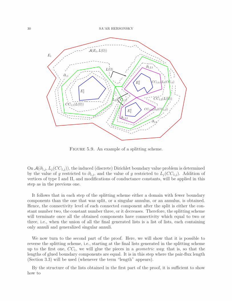
The complement of L(Ω), the maximal singular curve in Ω, has at most m-connectedcomponents, all of which, due to Proposition 5.3, have connectivity which is at most m− 1,or are annuli, or generalized singular annuli. By the maximum principle, one of these com-ponents has all of its vertices with g-values that are greater than the g-value along L(Ω). InSubsection 1.3, such a domain was denoted by O2(L(Ω)) and was called an exterior domain.Its boundary consists of E1 and L(Ω). It follows from Proposition 5.3 and Theorem 4.19that it is a generalized singular annulus which will be denoted by A(E1, L(Ω)).

A HARMONIC CONJUGATE 29

Let the full list of components of the complement of L(Ω) in Ω be enumerated as

(5.5) CC1 = CC1,1(L(Ω)), CC1,2(L(Ω)), . . . , CC1,p(L(Ω)) = A(E1, L(Ω)).

By definition, for each j = 1, . . . , p− 1, the g-value on the boundary component

(5.6) ∂1,j = ∂CC1,j(L(Ω)) ∩ L(Ω)

is the constant which equals the g-value on L(Ω). The other components of ∂CC1,j(L(Ω)),j = 1, . . . , p−1, are kept at g-values equal to 0. Hence, we now impose a (discrete) Dirichletboundary value problem with these values on each element in the list CC1 \ A(E1, L(Ω)).On A(E1, L(Ω)), the induced Dirichlet boundary value problem is determined by the valueof g restricted to E1 (which is equal to k), and the value of g restricted to L(Ω). Notethat imposing these boundary value problems in general will require introducing vertices oftype I and of type II and changing conductance constants along new edges, as describedin Subsection 1.3. These modifications are done in such a way that the restriction of theoriginal g solves the new boundary value problems.

For j = 1, . . . , p − 1, let kj denote the connectivity of CC1,j(L(Ω)). We now repeatthe procedure described in the first paragraph of the proof in each one of the connectedcomponents CC1,j(L(Ω)), at most kj − 2 times, for j = 1, . . . , p− 1, excluding those indicesthat correspond to annuli.

We will now describe the second step of the splitting scheme. For each j ∈ 1, . . . , p− 1whose corresponding component is not an annulus, a maximal singular level curve

(5.7) Lj(CC1,j) = L(CC1,j(L(Ω)))

with respect to the component CC1,j(L(Ω)), is chosen. This is possible because at the endof the previous step, we imposed a Dirichlet boundary value problem on each one of thesedomains. Hence, the assertions of Proposition 5.3 and Theorem 4.19 may be applied to thesedomains as well.

Therefore, a new list consisting of connected components of the complement of Lj(CC1,j)in CC1,j(L(Ω)), of cardinality at most m− 1,

(5.8) CC1,j = CC1,j,1(Lj(CC1,j)), CC1,j,2(Lj(CC1,j)), . . . , CC1,j,v(Lj(CC1,j)),

j as chosen above is generated. We will let the last element in this list denote the exteriordomain to Lj(CC1,j) in CC1,j. It is, as in the first step of the scheme, a generalized singularannulus denoted by A(∂1,j, Lj(CC1,j)). The other components have connectivity which is atmost (m − 2), or are annuli. Note that in this step the exterior domain from the first stepin the scheme, CC1,p(L(Ω)) = A(E1, L(Ω)), is left without any further splitting, since it is ageneralized singular annulus.

By definition, for each j chosen as above, and each i = 1, . . . v, the g-value on the boundarycomponent

(5.10) ∂1,j,i = ∂CC1,j,i(Lj(CC1,j)) ∩ Lj(CC1,j)

is the constant which equals the g-value on Lj(CC1,j). The other components of ∂CC1,j,i(L(Ω))are kept at g-values equal to 0. Hence, we now impose a (discrete) Dirichlet boundary valueproblem with the above values on each connected component in the list

(5.11) CC1,j \ A(∂1,j, Lj(CC1,j)).

30 SA’AR HERSONSKY

∂1,2,2

L(Ω)

CC1,1(L(Ω))

CC1,2(L(Ω))

∂1,2

∂1,1

CC1,2,1(L2(CC1,2)

CC1,2,2(L2(CC1,2))

E1

E12

E32

E22

L2(CC1,2)

A(E1, L(Ω))

∂1,2,1

Figure 5.9. An example of a splitting scheme.

OnA(∂1,j, Lj(CC1,j)), the induced (discrete) Dirichlet boundary value problem is determinedby the value of g restricted to ∂1,j, and the value of g restricted to Lj(CC1,j). Addition ofvertices of type I and II, and modifications of conductance constants, will be applied in thisstep as in the previous one.

It follows that in each step of the splitting scheme either a domain with fewer boundarycomponents than the one that was split, or a singular annulus, or an annulus, is obtained.Hence, the connectivity level of each connected component after the split is either the con-stant number two, the constant number three, or it decreases. Therefore, the splitting schemewill terminate once all the obtained components have connectivity which equal to two orthree, i.e., when the union of all the final generated lists is a list of lists, each containingonly annuli and generalized singular annuli.

We now turn to the second part of the proof. Here, we will show that it is possible toreverse the splitting scheme, i.e., starting at the final lists generated in the splitting schemeup to the first one, CC1, we will glue the pieces in a geometric way; that is, so that thelengths of glued boundary components are equal. It is in this step where the pair-flux length(Section 3.3) will be used (whenever the term “length” appears).

By the structure of the lists obtained in the first part of the proof, it is sufficient to showhow to

A HARMONIC CONJUGATE 31

(1) glue in a geometric way elements in a list, say CC1,j,...,kj , that contains only annuliand a generalized singular annuli so as to form a ladder of singular pair of pantsdenoted by S1,j,...,kj , and

(2) glue in a geometric way S1,j,...,kj to the singular boundary component of the general-ized singular annulus in the list from which CC1,j,...,kj was formed.

Note that, if all the elements in the list CC1,j,...,kj are annuli, we can apply case (2),since we will map each annulus via Theorem 0.5 to a Euclidean cylinder (by first applyingTheorem 0.5 and then Remark 4.33).

In order to ease the notation, let us show steps (1) and (2) for the lists produced in thefirst part of the proof.

Fix a j ∈ 1, . . . , p− 1, and for i = 1, . . . , v − 1, we apply Theorem 0.5 to

(5.12) Ai = CC1,j,i,

which by the assumption of step (1) is an annulus. This yields a collection of concentric Eu-clidean annuli S1, . . . , Sv−1 where, in the notation of Theorem 0.5, Si = SAi

. Furthermore,for each i = 1, . . . , v − 1, we have

(5.13) ri1, ri2 = 1, 2π Length(g,hi)

(L(∂1,j,i)) = 1, 2π exp( 2π

period(g∗i )g(∂1,j,i)

)

,

where g∗i is the period (Definition 2.19) of the conjugate function to g, the solution of theDirichlet boundary value problem defined on CC1,j,i.

We now apply the map F defined in Equation (4.29) to obtain a corresponding sequenceof Euclidean cylinders C1, . . . , Cv−1. All of these have radii equal to the constant 1, andtheir heights are given respectively by

(5.14) hi = log (2π Length(g,hi)(L(∂1,j,i))) = log 2π +

2π

period(g∗i )g(∂1,j,i).

Recall that the last component in the list CC1,j is the generalized singular annulusA(∂1,j, Lj(CC1,j)). Let h1,j be the conjugate harmonic function to g, the solution of theDirichlet boundary value problem induced on it (see the paragraph preceding Proposi-tion 4.22). Then, following Remark 4.33, we now map it to a generalized Euclidean cylinder,CA(∂1,j ,Lj(CC1,j)).

Measuring lengths of the image of the boundary components of A(∂1,j , Lj(CC1,j)) (using gand h1,j), which are in one to one correspondence with the singular boundary of this cylinder,yields the sequence of radii(5.15)

Ri =1

2π

Lengthg,hj(∂1,j,i)

Lengthg,hj(∂1,j)=

1

2π

1

period(g∗1,j)

exp(

2π

period(g∗i,j)g(∂1,j,i))

)

exp(

2π

period(g∗1,j)g(∂1,j)

)

∫

e∈∂1,j,i

|dh1,j(e)|,

for i = 1, . . . , v− 1, where the expression on the righthand side is based on Equation (3.21),and Equation (3.23). The sequence Ri, i = 1, . . . , v− 1 comprises the sequence of lengths ofthe round circles in the singular boundary component of CA(∂1,j , Lj(CC1,j)).

32 SA’AR HERSONSKY

Let

(5.16) fi = fRi= Riz

be the conformal homeomorphism acting on the Euclidean cylinder Ci = π F f(CC1,j,i),where z is the standard complex parameter on CC1,j,i. Hence, we may glue fi(Ci) alongone of its boundary components to the corresponding component in the singular boundarycomponent of CA(∂1,j ,Lj(CC1,j)), so that the length of the two boundaries are the same.

This establishes step (1).

We will now show how to establish step (2). The completion of step (1) yields a ladder ofsingular pairs of pants which we will denote by S1,j . This ladder has (m − 1) components;one corresponds to ∂1,j and the others comprise one boundary component of each one of thecylinders fi Ci, i = 1, . . .m − 2, after these cylinders are attached. Recall that ∂1,j is theintersection of the generalized singular annulus A(E1, L(Ω)), with the generalized singularannulus in the list CC1,j, which is A(∂1,j, Lj(CC1,j)).

Let g be the solution of the induced Dirichlet boundary value problem on A(E1, L(Ω)), andlet h be the harmonic conjugate function to g (see the paragraph preceding Proposition 4.22).Let

(5.17) τj =lj

Lengthg,h(∂i,j),

where lj denotes the length of the boundary component that corresponds to ∂1,j in S1,j ,and CA(E1,L(Ω)) is the generalized Euclidean cylinder constructed for A(E1, L(Ω)) (see Re-mark 4.33). After applying a conformal expansion of magnitude τj to S1,j, it then may beglued along this boundary component to CA(E1,L(Ω)) in such a way that the length of thecorresponding circle in the round bouquet ∂CA(E1,L(Ω)) has the same length. This establishesstep (2).

By construction, it is clear that the pair-flux length of the boundary component of SΩ

that corresponds to E1 is equal to

(5.18) 2π exp (2π

period(g∗)k),

where h is the harmonic conjugate to g, the solution of the Dirichelt boundary value probleminduced on A(E1, L(Ω)) (recall from Definition 1.6 that k is the value of g restricted to E1).The lengths of the remaining (m− 1) boundary components of SΩ, which correspond to them− 1 boundary components of E2, are determined by the process described in the previouspart of the proof.

The length of a component in SΩ which corresponds to Ei2, i ∈ 1, . . . , m− 1, measured

with respect to the pair-flux metric, is obtained by successively multiplying a sequence ofratios of lengths. These ratios are uniquely determined as in Equation (5.15), and Equa-tion (5.17), and present the expansion factor needed in order to match the gluing of a(generalized) cylinder to the one which induced it in the splitting process.

Cone angles are formed whenever more than two cylinders meet at a vertex; viewed in Ω,this will occur whenever more than two circles in a generalized bouquet meet at a vertex.The computation of the cone angles is solely determined by g and T . This analysis first

A HARMONIC CONJUGATE 33

appeared in Theorem 0.4 in [24]. Specifically, the cone angle φ(v) at a singular vertex v,which is the unique tangency point of n+ 1 Euclidean cylinders, satisfies

(5.19) φ(v) = 2(n+ 1)π.

The proof of the theorem is thus complete, with f defined to be the union of the individualmaps constructed at each stage.

References

[1] L. V. Ahlfors, Conformal invariants-Topics in Geometric Function Theory, McGraw-Hill Book Com-pany, 1973.

[2] E.M. Andreev, On convex polyhedra in Lobacevskii space, Mathematicheskii Sbornik (N.S.) 81 (123)(1970), 445–478 (Russian); Mathematics of the USSR-Sbornik 10 (1970), 413–440 (English).

[3] E.M. Andreev, On convex polyhedra of finite volume in Lobacevskii space, Mathematicheskii Sbornik(N.S.) 83 (125) (1970), 256–260 (Russian); Mathematics of the USSR-Sbornik 10 (1970), 255–259(English).

[4] T. Banchoff, Critical points and curvature for embedded polyhedra, J. Differential Geometry, 1 (1967),245–256.

[5] E. Bendito, A. Carmona, A.M. Encinas, Solving boundary value problems on networks using equilibrium

measures, J. of Func. Analysis, 171 (2000), 155–176.[6] E. Bendito, A. Carmona, A.M. Encinas, Shortest Paths in Distance-regular Graphs, Europ. J. Combi-

natorics, 21 (2000), 153–166.[7] E. Bendito, A. Carmona, A.M. Encinas, Equilibrium measure, Poisson Kernel and Effective Resistance

on Networks, De Gruyter. Proceeding in Mathematics, (V. Kaimanovich, K. Schmidt, W. Woess ed.),174 (2003), 363–376.

[8] E. Bendito, A. Carmona, A.M. Encinas, Difference schemes on uniform grids performed by general

discrete operators, Applied Numerical Mathematics, 50 (2004), 343–370.[9] I. Benjamini, O. Schramm, Random walks and harmonic functions on infinite planar graphs using square

tilings, Ann. Probab. 24 (1996), 1219–1238.[10] I. Benjamini, O. Schramm, Harmonic functions on planar and almost planar graphs and manifolds, via

circle packings, Invent. Math. 126 (1996), 565–587.[11] R.L Brooks, C.A. Smith, A.B. Stone and W.T. Tutte, The dissection of squares into squares, Duke

Math. J. 7 (1940), 312–340.[12] J. W. Cannon, The combinatorial Riemann mapping theorem, Acta Math. 173 (1994), 155–234.[13] J.W. Cannon, W.J. Floyd and W.R. Parry, Squaring rectangles: the finite Riemann mapping theorem,

Contemporary Mathematics, Amer. Math. Soc., vol. 169, Providence, 1994, 133–212.[14] D. Chelkak and S. Smirnov, Discrete complex analysis on isoradial graphs, Adv. Math. 228 (2011),

1590-1630.[15] F.R. Chung, A. Grigoryan and S.T. Yau, Upper bounds for eigenvalues of the discrete and continuous

Laplace operators, Adv. Math. 117 (1996), 165–178.

[16] R. Courant, K. Friedrichs and H. Lewy, Uber die partiellen Differenzengleichungen der mathematischen

Physic, Math. Ann 100 (1928), 32 – 74.[17] M. Dehn, Zerlegung ovn Rechtecke in Rechtecken, Mathematische Annalen, 57, (1903), 144-167.[18] R. Duffin, The extremal length of a network, J. Math. Anal. Appl. 5 (1962), 200–215.[19] B. Fuglede, On the theory of potentials in locally compact spaces, Acta. Math. 103 (1960), 139–215.[20] D. Glickenstein.Discrete conformal variations and scalar curvature on piecewise flat two- and three-

dimensional manifolds, J. Differential Geom. 87 (2011), 201–237.[21] G.X. David, F. Luo and S.H. Yau, Recent advances in computational conformal geometry, Commun.

Inf. Syst. 9 (2009), 163–195.

34 SA’AR HERSONSKY

[22] G.X. David, F. Luo, Z. Wei and S.H. Yau, Numerical computation of surface conformal mappings,Comput. Methods Funct. Theory 11 (2011), 747–787.

[23] S. Hersonsky, Energy and length in a topological planar quadrilateral, Euro. Jour. of Combinatorics 29(2008), 208-217.

[24] S. Hersonsky, Boundary Value Problems on Planar Graphs and Flat Surfaces with Integer Cone singu-

larities I; The Dirichlet problem, J. Reine Angew. Math. 670, (2012), 65–92.[25] S. Hersonsky, Boundary Value Problems on Planar Graphs and Flat Surfaces with Integer Cone singu-

larities II; Dirichlet-Neumann problem, Differential Geometry and its Applications 29 (2011), 329–347.[26] S. Hersonsky, Combinatorial Harmonic Maps and Convergence to Conformal Maps, II: Convergence

and Moduli., in preparation.[27] A.N. Hirani, Discrete exterior calculus, Dissertation (Ph.D.), California Institute of Technology,

http://resolver.caltech.edu/CaltechETD:etd-05202003-095403.[28] R. Kenyon, Tilings and discrete Dirichlet problems, Israel J. Math. 105 (1998), 61–84.[29] P. Koebe, Uber die Unifirmiseriung beliegiger analytischer Kurven III, Nachrichten Gesellschaft fur

Wisseenschaften in Gottingen (1908), 337–358.[30] P. Koebe, Kontaktprobleme der Konformen Abbildung, Ber. Sachs. Akad. Wiss. Leipzig, Math.-Phys.

Kl. 88 (1936) 141–164.[31] F. Lazarus and A. Verroust, Level Set Diagrams of Polyhedral Objects, ACM Symposium on Solid and

Physical Modeling, Ann Arbor, Michigan, (1999), 130–140.[32] F. Luo, Variational principles on triangulated surfaces, Handbook of geometric analysis. No. 1, 259276,

Adv. Lect. Math. (ALM), 7, Int. Press, Somerville, MA, 2008.[33] C. Mercat, Discrete Riemann surfaces, Handbook of Teichmuller theory. Vol. I, 541575, IRMA Lect.

Math. Theor. Phys., 11, Eur. Math. Soc., Zurich, 2007.[34] K. Polthier, Computational aspects of discrete minimal surfaces, Global theory of minimal surfaces,

65111, Clay Math. Proc., 2, Amer. Math. Soc., Providence, RI, 2005.[35] B. Rodin and D. Sullivan, The convergence of circle packing to the Riemann mapping, Jour. Differential

Geometry 26 (1987), 349–360.[36] C.T. Sass, K. Stephenson and W.G. Brock, Circle packings on conformal and affine tori, Computational

algebraic and analytic geometry, 211–220, Contemp. Math., 572, Amer. Math. Soc., Providence, RI,2012.

[37] O. Schramm, Square tilings with prescribed combinatorics, Israel Jour. of Math. 84 (1993), 97–118.[38] P.M. Soardi, Potential theory on infinite networks, Lecture Notes in Mathematics, 1590, Springer-Verlag

Berlin Heidelberg 1994.[39] G. Springer, Introduction to Riemann surfaces, Addison-Wesley Publishing Company, Inc., Reading,

Mass. 1957.[40] K. Stephenson, A Probabilistic Proof of Thurston’s Conjecture on Circle Packings, Rendiconti del Sem-

inario Mate. e Fisico di Milano, LXVI (1996), 201–291.[41] W.P. Thurston, The finite Riemann mapping theorem, invited address, International Symposium in

Celebration of the Proof of the Bieberbach Conjecture, Purdue University, 1985.[42] W.P. Thurston, The Geometry and Topology of 3-manifolds, Princeton University Notes, Princeton,

New Jersey, 1982.

Department of Mathematics, University of Georgia, Athens, GA 30602

URL: http://www.math.uga.edu/~saarhE-mail address : saarh@math.uga.edu