Projection Methods

Jesús Fernández-Villaverde

University of Pennsylvania

July 10, 2011

Jesús Fernández-Villaverde (PENN) Projection Methods July 10, 2011 1 / 52

Introduction

Introduction

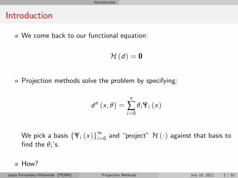
We come back to our functional equation:

H (d) = 0

Projection methods solve the problem by specifying:

dn (x , θ) =n

∑i=0

θiΨi (x)

We pick a basis fΨi (x)g∞i=0 and projectH () against that basis to

nd the θis.

How?

Jesús Fernández-Villaverde (PENN) Projection Methods July 10, 2011 2 / 52

Introduction

Points to Emphasize

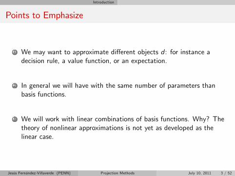
1 We may want to approximate di¤erent objects d : for instance adecision rule, a value function, or an expectation.

2 In general we will have with the same number of parameters thanbasis functions.

3 We will work with linear combinations of basis functions. Why? Thetheory of nonlinear approximations is not yet as developed as thelinear case.

Jesús Fernández-Villaverde (PENN) Projection Methods July 10, 2011 3 / 52

Introduction

Basic Algorithm

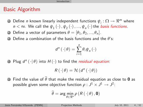
1 Dene n known linearly independent functions ψi : Ω ! <m wheren < ∞. We call the ψ1 () ,ψ2 () , ...,ψn () the basis functions.

2 Dene a vector of parameters θ = [θ1, θ2, ..., θn ].3 Dene a combination of the basis functions and the θs:

dn ( j θ) =n

∑i=1

θiψn ()

4 Plug dn ( j θ) into H () to nd the residual equation:

R ( j θ) = H (dn ( j θ))

5 Find the value of bθ that make the residual equation as close to 0 aspossible given some objective function ρ : J1 J1 ! J2:bθ = arg min

θ2<nρ (R ( j θ) , 0)

Jesús Fernández-Villaverde (PENN) Projection Methods July 10, 2011 4 / 52

Introduction

Relation with Econometrics

Looks a lot like OLS. Explore this similarity later in more detail.

Also with semi-nonparametric methods as Sieves.

Compare with:

1 Policy iteration.

2 Parameterized Expectations.

Jesús Fernández-Villaverde (PENN) Projection Methods July 10, 2011 5 / 52

Introduction

Two Issues

We need to decide:

1 Which basis we use?

1 Pick a global basis)spectral methods.

2 Pick a local basis)nite elements methods.

2 How do we project?

Di¤erent choices in 1 and 2 will result in slightly di¤erent projectionmethods.

Jesús Fernández-Villaverde (PENN) Projection Methods July 10, 2011 6 / 52

Introduction

Spectral Methods

Main reference: Judd (1992).

Spectral techniques use basis functions that are nonzero and smoothalmost everywhere in Ω.

Advantages: simplicity.

Disadvantages: di¢ cult to capture local behavior. Gibbs phenomenon.

Jesús Fernández-Villaverde (PENN) Projection Methods July 10, 2011 7 / 52

Introduction

Spectral Basis I

Monomials: c , x , x2, x3, ...

Simple and intuitive.Even if this basis is not composed by orthogonal functions, if J1 is thespace of bounded measurable functions on a compact set, theStone-Weierstrass theorem assures completeness in the L1 norm.Problems:

1 (Nearly) multicollinearity. Compare the graph of x10 with x11.The solution of a projection involves matrices inversion. When thebasis functions are similar, the condition number of these matrices (theratio of the largest and smallest absolute eigenvalues) are too high.Just the six rst monomials can generate conditions numbers of 1010.The matrix of the LS problem of tting a polynomial of degree 6 to afunction (the Hilbert Matrix), is a popular test of numerical accuracysince it maximizes rounding errors!

2 Monomials vary considerably in size, leading to scaling problems andaccumulation of numerical errors.

We want an orthogonal basis.Jesús Fernández-Villaverde (PENN) Projection Methods July 10, 2011 8 / 52

Introduction

Spectral Basis II

Trigonometric series

1/ (2π)0.5 , cos x/ (2π)0.5 , sin x/ (2π)0.5 , ...,

cos kx/ (2π)0.5 , sin kx/ (2π)0.5 , ...

Periodic functions.

However economic problems are generally not periodic.

Periodic approximations to nonperiodic functions su¤er from theGibbs phenomenon, requiring many terms to achieve good numericalperformance (the rate of convergence to the true solution as n! ∞is only O (n)).

Jesús Fernández-Villaverde (PENN) Projection Methods July 10, 2011 9 / 52

Introduction

Spectral Basis III

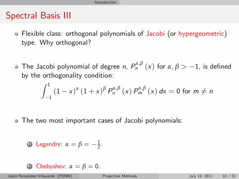
Flexible class: orthogonal polynomials of Jacobi (or hypergeometric)type. Why orthogonal?

The Jacobi polynomial of degree n, Pα,βn (x) for α, β > 1, is dened

by the orthogonality condition:Z 1

1(1 x)α (1+ x)β Pα,β

n (x)Pα,βm (x) dx = 0 for m 6= n

The two most important cases of Jacobi polynomials:

1 Legendre: α = β = 12 .

2 Chebyshev: α = β = 0.Jesús Fernández-Villaverde (PENN) Projection Methods July 10, 2011 10 / 52

Introduction

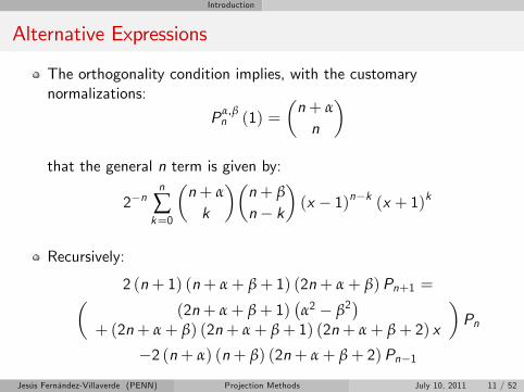
Alternative Expressions

The orthogonality condition implies, with the customarynormalizations:

Pα,βn (1) =

n+ α

n

that the general n term is given by:

2nn

∑k=0

n+ α

k

n+ β

n k

(x 1)nk (x + 1)k

Recursively:

2 (n+ 1) (n+ α+ β+ 1) (2n+ α+ β)Pn+1 =(2n+ α+ β+ 1)

α2 β2

+ (2n+ α+ β) (2n+ α+ β+ 1) (2n+ α+ β+ 2) x

Pn

2 (n+ α) (n+ β) (2n+ α+ β+ 2)Pn1

Jesús Fernández-Villaverde (PENN) Projection Methods July 10, 2011 11 / 52

Introduction

Chebyshev Polynomials

One of the most common tools of Applied Mathematics.

References:

Chebyshev and Fourier Spectral Methods, John P. Boyd (2001).

A Practical Guide to Pseudospectral Methods, Bengt Fornberg (1998).

Advantages of Chebyshev Polynomials:

1 Numerous simple close-form expressions are available.2 The change between the coe¢ cients of a Chebyshev expansion of afunction and the values of the function at the Chebyshev nodes arequickly performed by the cosine transform.

3 They are more robust than their alternatives for interpolation.4 They are bounded between [1, 1] while Legendre polynomials are not,o¤ering a better performance close to the boundaries of the problems.

5 They are smooth functions.6 Several theorems bound the errors for Chebyshev polynomialsinterpolations.

Jesús Fernández-Villaverde (PENN) Projection Methods July 10, 2011 12 / 52

Introduction

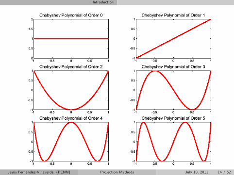
Denition of Chebyshev Polynomials I

Recursive denition:

T0 (x) = 1

T1 (x) = x

Tn+1 (x) = 2xTn (x) Tn1 (x) for a general n

The rst few polynomials are then 1, x , 2x2 1, 4x3 3x ,8x4 8x2 + 1, etc...

The n zeros of the polynomial Tn (xk ) = 0 are given by:

xk = cos2k 12n

π, k = 1, ..., n

Note that zeros are clustered quadratically towards 1.Jesús Fernández-Villaverde (PENN) Projection Methods July 10, 2011 13 / 52

Introduction

Jesús Fernández-Villaverde (PENN) Projection Methods July 10, 2011 14 / 52

Introduction

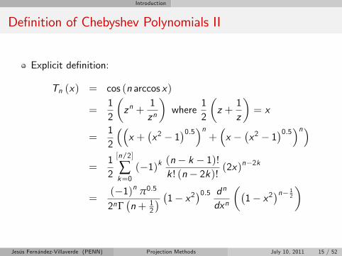
Denition of Chebyshev Polynomials II

Explicit denition:

Tn (x) = cos (n arccos x)

=12

zn +

1zn

where

12

z +

1z

= x

=12

x +

x2 1

0.5n+x

x2 1

0.5n=

12

[n/2]

∑k=0

(1)k (n k 1)!k ! (n 2k)! (2x)

n2k

=(1)n π0.5

2nΓn+ 1

2

1 x20.5 dndxn

1 x2

n 12

Jesús Fernández-Villaverde (PENN) Projection Methods July 10, 2011 15 / 52

Introduction

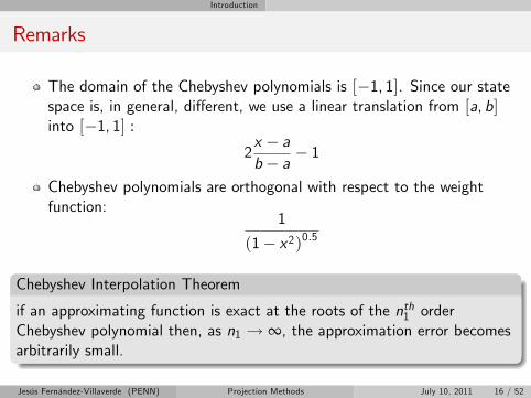
Remarks

The domain of the Chebyshev polynomials is [1, 1]. Since our statespace is, in general, di¤erent, we use a linear translation from [a, b]into [1, 1] :

2x ab a 1

Chebyshev polynomials are orthogonal with respect to the weightfunction:

1

(1 x2)0.5

Chebyshev Interpolation Theorem

if an approximating function is exact at the roots of the nth1 orderChebyshev polynomial then, as n1 ! ∞, the approximation error becomesarbitrarily small.

Jesús Fernández-Villaverde (PENN) Projection Methods July 10, 2011 16 / 52

Introduction

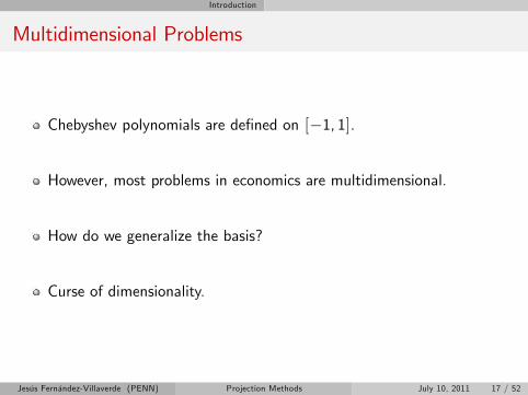
Multidimensional Problems

Chebyshev polynomials are dened on [1, 1].

However, most problems in economics are multidimensional.

How do we generalize the basis?

Curse of dimensionality.

Jesús Fernández-Villaverde (PENN) Projection Methods July 10, 2011 17 / 52

Introduction

Tensors

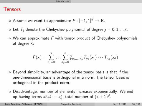
Assume we want to approximate F : [1, 1]d ! R.

Let Tj denote the Chebyshev polynomial of degree j = 0, 1, .., κ.

We can approximate F with tensor product of Chebyshev polynomialsof degree κ:

F (x) =κ

∑n1=0

. . .κ

∑nd=0

ξn1,...,ndTn1(x1) Tnd (xd )

Beyond simplicity, an advantage of the tensor basis is that if theone-dimensional basis is orthogonal in a norm, the tensor basis isorthogonal in the product norm.

Disadvantage: number of elements increases exponentially. We endup having terms xκ

1 xκ2 xκ

d , total number of (κ + 1)d .

Jesús Fernández-Villaverde (PENN) Projection Methods July 10, 2011 18 / 52

Introduction

Complete Polynomials

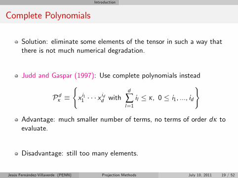
Solution: eliminate some elements of the tensor in such a way thatthere is not much numerical degradation.

Judd and Gaspar (1997): Use complete polynomials instead

Pdκ (x i11 x

idd with

d

∑l=1

il κ, 0 i1, ..., id

)

Advantage: much smaller number of terms, no terms of order dκ toevaluate.

Disadvantage: still too many elements.

Jesús Fernández-Villaverde (PENN) Projection Methods July 10, 2011 19 / 52

Introduction

Smolyaks Algorithm I

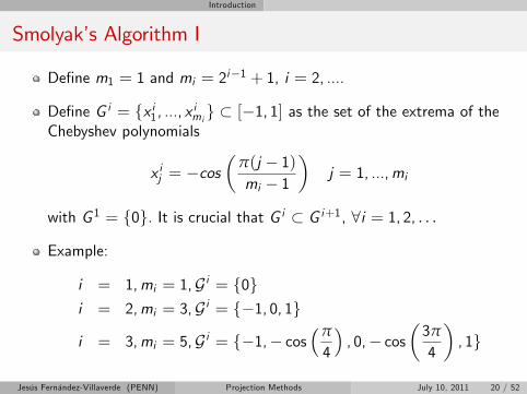
Dene m1 = 1 and mi = 2i1 + 1, i = 2, ....

Dene G i = fx i1, ..., x imi g [1, 1] as the set of the extrema of theChebyshev polynomials

x ij = cos

π(j 1)mi 1

j = 1, ...,mi

with G 1 = f0g. It is crucial that G i G i+1, 8i = 1, 2, . . .

Example:

i = 1,mi = 1,G i = f0gi = 2,mi = 3,G i = f1, 0, 1g

i = 3,mi = 5,G i = f1, cosπ

4

, 0, cos

3π

4

, 1g

Jesús Fernández-Villaverde (PENN) Projection Methods July 10, 2011 20 / 52

Introduction

Smolyaks Algorithm II

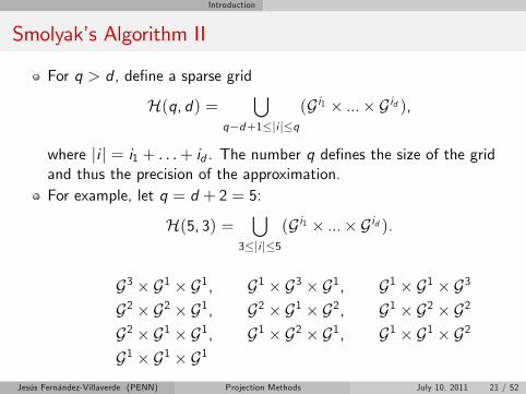
For q > d , dene a sparse grid

H(q, d) =[

qd+1ji jq(G i1 ... G id ),

where ji j = i1 + . . .+ id . The number q denes the size of the gridand thus the precision of the approximation.For example, let q = d + 2 = 5:

H(5, 3) =[

3ji j5(G i1 ... G id ).

G3 G1 G1, G1 G3 G1, G1 G1 G3

G2 G2 G1, G2 G1 G2, G1 G2 G2

G2 G1 G1, G1 G2 G1, G1 G1 G2

G1 G1 G1

Jesús Fernández-Villaverde (PENN) Projection Methods July 10, 2011 21 / 52

Introduction

Smolyaks Algorithm III

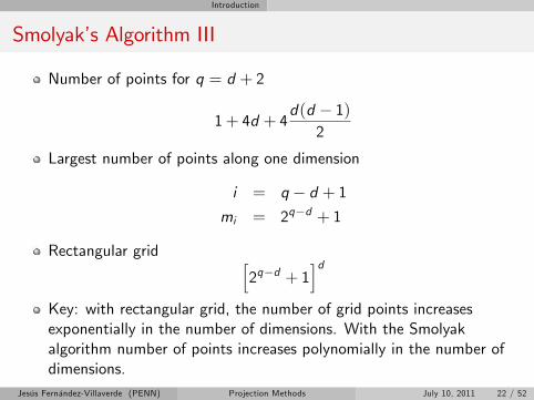
Number of points for q = d + 2

1+ 4d + 4d(d 1)

2

Largest number of points along one dimension

i = q d + 1mi = 2qd + 1

Rectangular grid h2qd + 1

idKey: with rectangular grid, the number of grid points increasesexponentially in the number of dimensions. With the Smolyakalgorithm number of points increases polynomially in the number ofdimensions.

Jesús Fernández-Villaverde (PENN) Projection Methods July 10, 2011 22 / 52

Introduction

Smolyaks Algorithm IV

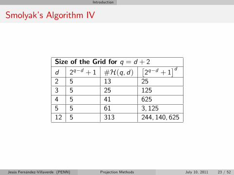
Size of the Grid for q = d + 2d 2qd + 1 #H(q, d)

2qd + 1

d2 5 13 253 5 25 1254 5 41 6255 5 61 3, 12512 5 313 244, 140, 625

Jesús Fernández-Villaverde (PENN) Projection Methods July 10, 2011 23 / 52

Introduction

Smolyaks Algorithm V

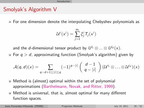
For one dimension denote the interpolating Chebyshev polynomials as

U i (x i ) =mi

∑j=1

ξ ijTj (xi )

and the d-dimensional tensor product by U i1 ... U id (x).For q > d , approximating function (Smolyaks algorithm) given by

A(q, d)(x) = ∑qd+1ji jq

(1)qji jd 1q ji j

(U i1 . . .U id )(x)

Method is (almost) optimal within the set of polynomialapproximations (Barthelmann, Novak, and Ritter, 1999).

Method is universal, that is, almost optimal for many di¤erentfunction spaces.

Jesús Fernández-Villaverde (PENN) Projection Methods July 10, 2011 24 / 52

Introduction

Boyds Moral Principal

1 When in doubt, use Chebyshev polynomials unless the solution isspatially periodic, in which case an ordinary Fourier series is better.

2 Unless you are sure another set of basis functions is better, useChebyshev polynomials.

3 Unless you are really, really sure another set of basis functions isbetter, use Chebyshev polynomials.

Jesús Fernández-Villaverde (PENN) Projection Methods July 10, 2011 25 / 52

Introduction

Finite Elements

Standard Reference: McGrattan (1999).

Bound the domain Ω in small of the state variables.

Partition Ω in small in nonintersecting elements.

These small sections are called elements.

The boundaries of the elements are called nodes.

Jesús Fernández-Villaverde (PENN) Projection Methods July 10, 2011 26 / 52

Introduction

Partition into Elements

Elements may be of unequal size.

We can have small elements in the areas of Ω where the economy willspend most of the time while just a few, big size elements will coverwide areas of the state space infrequently visited.

Also, through elements, we can easily handle issues like kinks orconstraints.

There is a whole area of research concentrated on the optimalgeneration of an element grid. See Thomson, Warsi, and Mastin(1985).

Jesús Fernández-Villaverde (PENN) Projection Methods July 10, 2011 27 / 52

Introduction

Structure

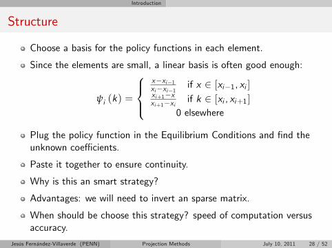
Choose a basis for the policy functions in each element.

Since the elements are small, a linear basis is often good enough:

ψi (k) =

8><>:xxi1xixi1 if x 2 [xi1, xi ]xi+1xxi+1xi if k 2 [xi , xi+1]

0 elsewhere

Plug the policy function in the Equilibrium Conditions and nd theunknown coe¢ cients.

Paste it together to ensure continuity.

Why is this an smart strategy?

Advantages: we will need to invert an sparse matrix.

When should be choose this strategy? speed of computation versusaccuracy.

Jesús Fernández-Villaverde (PENN) Projection Methods July 10, 2011 28 / 52

Introduction

Three Di¤erent Renements

1 h-renement: subdivide each element into smaller elements toimprove resolution uniformly over the domain.

2 r-renement: subdivide each element only in those regions wherethere are high nonlinearities.

3 p-renement: increase the order of the approximation in eachelement. If the order of the expansion is high enough, we willgenerate in that way an hybrid of nite and spectral methods knowsas spectral elements.

Jesús Fernández-Villaverde (PENN) Projection Methods July 10, 2011 29 / 52

Introduction

Choosing the Objective Function

The most common answer to the second question is given by aweighted residual.

That is why often projection methods are also called weightedresidual methods

This set of techniques propose to get the residual close to 0 in theweighted integral sense.

Given some weight functions φi : Ω ! <m :

ρ (R ( j θ) , 0) =0 if

RΩ φi (x)R ( j θ) dx = 0, i = 1, .., n

1 otherwise

Then the problem is to choose the θ that solve the system ofequations: Z

Ωφi (x)R ( j θ) dx = 0, i = 1, .., n

Jesús Fernández-Villaverde (PENN) Projection Methods July 10, 2011 30 / 52

Introduction

Remarks

With the approximation of d by some functions ψi and the denitionof some weight functions φi (), we have transform a ratherintractable functional equation problem into the standard nonlinearequations system!

The solution of this system can be found using standard methods, asa Newton for relatively small problems or a conjugate gradient forbigger ones.

Issue: we have di¤erent choices for an weight function:

Jesús Fernández-Villaverde (PENN) Projection Methods July 10, 2011 31 / 52

Introduction

Weight Function I: Least Squares

φi (x) =∂R ( x jθ)

∂θi.

This choice is motivated by the solution of the variational problem:

minθ

ZΩR2 ( j θ) dx

with rst order condition:ZΩ

∂R (x j θ)∂θi

R ( j θ) dx = 0, i = 1, .., n

Variational problem is mathematically equivalent to a standardregression problem in econometrics.

OLS or NLLS are regression against a manifold spanned by theobservations.

Jesús Fernández-Villaverde (PENN) Projection Methods July 10, 2011 32 / 52

Introduction

Weight Function I: Least Squares

Least Squares always generates symmetric matrices even if theoperator H is not self-adjoint.

Symmetric matrices are convenient theoretically (they simplify theproofs) and computationally (there are algorithms that exploit theirstructure to increase speed and decrease memory requirements).

However, least squares may lead to ill-conditioning and systems ofequations complicated to solve numerically.

Jesús Fernández-Villaverde (PENN) Projection Methods July 10, 2011 33 / 52

Introduction

Weight Function II: Subdomain

We divide the domain Ω in n subdomains Ωi and dene the n stepfunctions:

φi (x) =1 if x 2 Ωi

0 otherwise

This choice is then equivalent to solve the system:ZΩi

R ( j θ) dx = 0, i = 1, .., n

Jesús Fernández-Villaverde (PENN) Projection Methods July 10, 2011 34 / 52

Introduction

Weight Function III: Moments

Take0, x , x2, ..., xn1

and compute the rst n periods of the

residual function: ZΩi

x iR ( j θ) dx = 0, i = 0, .., n

This approach, widely used in engineering works well for a low n (2 or3).

However, for higher orders, its numerical performance is very low:high orders of x are highly collinear and arise serious rounding errorproblems.

Hence, moments are to be avoided as weight functions.

Jesús Fernández-Villaverde (PENN) Projection Methods July 10, 2011 35 / 52

Introduction

Weight Function III: Collocation or Pseudospectral orMethod of Selected Points

φi (x) = δ (x xi ) where δ is the dirac delta function and xi are thecollocation points.This method implies that the residual function is zero at the ncollocation points.Simple to compute since the integral only needs to be evaluated inone point. Specially attractive when dealing with strong nonlinearities.A systematic way to pick collocation points is to use a densityfunction:

µγ (x) =Γ 32 γ

(1 x2)γ π

12 Γ (1 γ)

γ < 1

and nd the collocation points as the xj , j = 0, ..., n 1 solutions to:Z xj

1µγ (x) dx =

jn

For γ = 0, the density function implies equispaced points.Jesús Fernández-Villaverde (PENN) Projection Methods July 10, 2011 36 / 52

Introduction

Weight Function IV: Orthogonal Collocation

Variation of the collocation method:

1 Basis functions are a set of orthogonal polynomials.

2 Collocation points given by the roots of the n th polynomial.

When we use Chebyshev polynomials, their roots are the collocationpoints implied by µ 1

2(x) and their clustering can be shown to be

optimal as n! ∞.

Surprisingly good performance of orthogonal collocation methods.

Jesús Fernández-Villaverde (PENN) Projection Methods July 10, 2011 37 / 52

Introduction

Weight Function V: Galerkin or Rayleigh-Ritz

φi (x) = ψi (x) with a linear approximating function ∑ni=1 θiψi (x).

Then: ZΩ

ψi (x)H

n

∑i=1

θiψi (x)

!dx = 0, i = 1, .., n

that is, the residual has to be orthogonal to each of the basisfunctions.Galerkin is a highly accurate and robust but di¢ cult to code.If the basis functions are complete over J1 (they are indeed a basis ofthe space), then the Galerkin solution will converge pointwise to thetrue solution as n goes to innity:

limn!∞

n

∑i=1

θiψi () = d ()

Experience suggests that a Galerkin approximation of order n is asaccurate as a Pseudospectral n+ 1 or n+ 2 expansion.

Jesús Fernández-Villaverde (PENN) Projection Methods July 10, 2011 38 / 52

Introduction

A Simple Example

Imagine that the law of motion for the price x of a good is given by:

d 0 (x) + d (x) = 0

Let us apply a simple projection to solve this di¤erential equation.

Code: test.m, test2.m, test3.m

Jesús Fernández-Villaverde (PENN) Projection Methods July 10, 2011 39 / 52

Introduction

Analysis of Error

As with projection, it is important to study the Euler equation errors.

We can improve errors:

1 Adding additional functions in the basis.

2 Rene the elements.

Multigrid schemes.

Jesús Fernández-Villaverde (PENN) Projection Methods July 10, 2011 40 / 52

Introduction

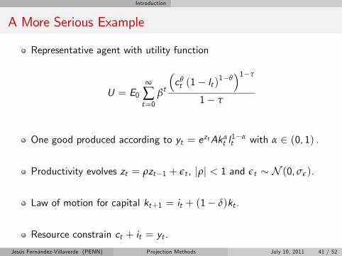
A More Serious Example

Representative agent with utility function

U = E0∞

∑t=0

βt

cθt (1 lt )

1θ1τ

1 τ

One good produced according to yt = eztAkαt l1αt with α 2 (0, 1) .

Productivity evolves zt = ρzt1 + εt , jρj < 1 and εt N (0, σε).

Law of motion for capital kt+1 = it + (1 δ)kt .

Resource constrain ct + it = yt .

Jesús Fernández-Villaverde (PENN) Projection Methods July 10, 2011 41 / 52

Introduction

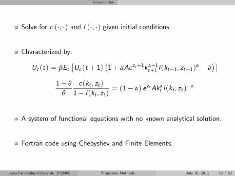
Solve for c (, ) and l (, ) given initial conditions.

Characterized by:

Uc (t) = βEtUc (t + 1)

1+ αAezt+1kα1

t+1 l(kt+1, zt+1)α δ

1 θ

θ

c(kt , zt )1 l(kt , zt )

= (1 α) eztAkαt l(kt , zt )

α

A system of functional equations with no known analytical solution.

Fortran code using Chebyshev and Finite Elements.

Jesús Fernández-Villaverde (PENN) Projection Methods July 10, 2011 42 / 52

Introduction

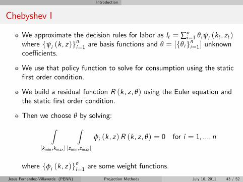
Chebyshev I

We approximate the decision rules for labor as lt = ∑ni=1 θiψi (kt , zt )

where fψi (k, z)gni=1 are basis functions and θ = [fθigni=1] unknown

coe¢ cients.

We use that policy function to solve for consumption using the staticrst order condition.

We build a residual function R (k, z , θ) using the Euler equation andthe static rst order condition.

Then we choose θ by solving:Z[kmin,kmax ]

Z[zmin,zmax ]

φi (k, z)R (k, z , θ) = 0 for i = 1, ..., n

where fφi (k, z)gni=1 are some weight functions.

Jesús Fernández-Villaverde (PENN) Projection Methods July 10, 2011 43 / 52

Introduction

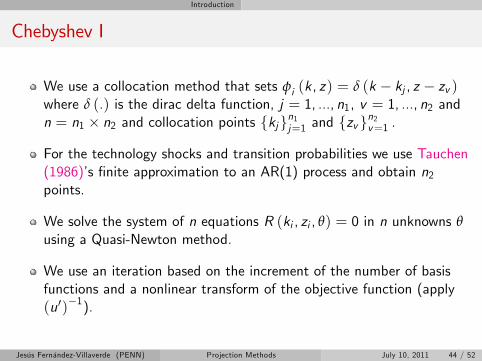
Chebyshev I

We use a collocation method that sets φi (k, z) = δ (k kj , z zv )where δ (.) is the dirac delta function, j = 1, ..., n1, v = 1, ..., n2 andn = n1 n2 and collocation points fkjgn1j=1 and fzv g

n2v=1 .

For the technology shocks and transition probabilities we use Tauchen(1986)s nite approximation to an AR(1) process and obtain n2points.

We solve the system of n equations R (ki , zi , θ) = 0 in n unknowns θusing a Quasi-Newton method.

We use an iteration based on the increment of the number of basisfunctions and a nonlinear transform of the objective function (apply(u0)1).

Jesús Fernández-Villaverde (PENN) Projection Methods July 10, 2011 44 / 52

Introduction

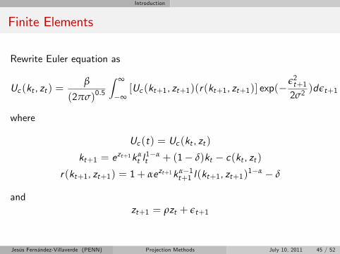
Finite Elements

Rewrite Euler equation as

Uc (kt , zt ) =β

(2πσ)0.5

Z ∞

∞[Uc (kt+1, zt+1)(r(kt+1, zt+1)] exp(

ε2t+12σ2

)dεt+1

where

Uc (t) = Uc (kt , zt )

kt+1 = ezt+1kαt l1αt + (1 δ)kt c(kt , zt )

r(kt+1, zt+1) = 1+ αezt+1kα1t+1 l(kt+1, zt+1)

1α δ

andzt+1 = ρzt + εt+1

Jesús Fernández-Villaverde (PENN) Projection Methods July 10, 2011 45 / 52

Introduction

Goal

The problem is to nd two policy functionsc(k, z) : R+ [0,∞]! R+ and l(k, z) : R+ [0,∞]! [0, 1] thatsatisfy the model equilibrium conditions.

Since the static rst order condition gives a relation between the twopolicy functions, we only need to solve for one of them.

For the rest of the exposition we will assume that we actually solvefor l(k, z) and then we nd c (l(k, z)).

Jesús Fernández-Villaverde (PENN) Projection Methods July 10, 2011 46 / 52

Introduction

Bounding the State Space I

We bound the domain of the state variables to partition it innonintersecting elements.

To bound the productivity level of the economy dene λt = tanh(zt ).

Since λt 2 [1, 1] we can write the stochastic process as:

λt = tanh(ρ tanh1(zt1) + 20.5σvt )

where vt = εt20.5σ

.

Jesús Fernández-Villaverde (PENN) Projection Methods July 10, 2011 47 / 52

Introduction

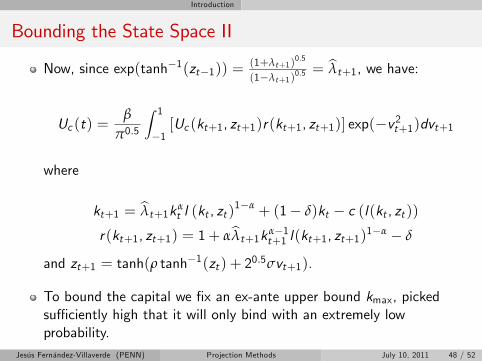
Bounding the State Space II

Now, since exp(tanh1(zt1)) =(1+λt+1)

0.5

(1λt+1)0.5 = bλt+1, we have:

Uc (t) =β

π0.5

Z 1

1[Uc (kt+1, zt+1)r(kt+1, zt+1)] exp(v2t+1)dvt+1

where

kt+1 = bλt+1kαt l (kt , zt )

1α + (1 δ)kt c (l(kt , zt ))r(kt+1, zt+1) = 1+ αbλt+1kα1

t+1 l(kt+1, zt+1)1α δ

and zt+1 = tanh(ρ tanh1(zt ) + 20.5σvt+1).

To bound the capital we x an ex-ante upper bound kmax, pickedsu¢ ciently high that it will only bind with an extremely lowprobability.

Jesús Fernández-Villaverde (PENN) Projection Methods July 10, 2011 48 / 52

Introduction

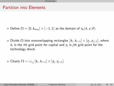
Partition into Elements

Dene Ω = [0, kmax] [1, 1] as the domain of lfe (k, z ; θ).

Divide Ω into nonoverlapping rectangles [ki , ki+1] [zj , zj+1], whereki is the ith grid point for capital and zj is jth grid point for thetechnology shock.

Clearly Ω = [i ,j [ki , ki+1] [zj , zj+1].

Jesús Fernández-Villaverde (PENN) Projection Methods July 10, 2011 49 / 52

Introduction

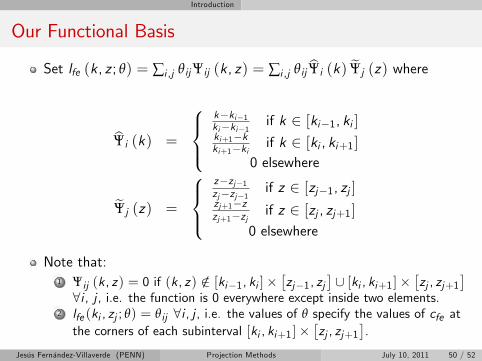
Our Functional Basis

Set lfe (k, z ; θ) = ∑i ,j θijΨij (k, z) = ∑i ,j θij bΨi (k) eΨj (z) where

bΨi (k) =

8><>:kki1kiki1 if k 2 [ki1, ki ]ki+1kki+1ki if k 2 [ki , ki+1]

0 elsewhere

eΨj (z) =

8><>:zzj1zjzj1 if z 2 [zj1, zj ]zj+1zzj+1zj if z 2 [zj , zj+1]

0 elsewhere

Note that:1 Ψij (k, z) = 0 if (k, z) /2 [ki1, ki ]

zj1, zj

[ [ki , ki+1 ]

zj , zj+1

8i , j , i.e. the function is 0 everywhere except inside two elements.

2 lfe (ki , zj ; θ) = θij 8i , j , i.e. the values of θ specify the values of cfe atthe corners of each subinterval [ki , ki+1 ]

zj , zj+1

.

Jesús Fernández-Villaverde (PENN) Projection Methods July 10, 2011 50 / 52

Introduction

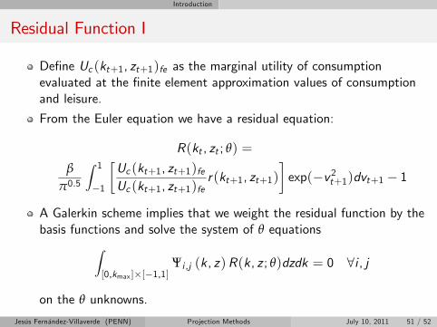
Residual Function I

Dene Uc (kt+1, zt+1)fe as the marginal utility of consumptionevaluated at the nite element approximation values of consumptionand leisure.

From the Euler equation we have a residual equation:

R(kt , zt ; θ) =

β

π0.5

Z 1

1

Uc (kt+1, zt+1)feUc (kt+1, zt+1)fe

r(kt+1, zt+1)exp(v2t+1)dvt+1 1

A Galerkin scheme implies that we weight the residual function by thebasis functions and solve the system of θ equationsZ

[0,kmax ][1,1]Ψi ,j (k, z)R(k, z ; θ)dzdk = 0 8i , j

on the θ unknowns.

Jesús Fernández-Villaverde (PENN) Projection Methods July 10, 2011 51 / 52

Introduction

Residual Function II

Since Ψij (k, z) = 0 if(k, z) /2 [ki1, ki ] [zj1, zj ] [ [ki , ki+1] [zj , zj+1] 8i , j we haveZ[ki1,ki ][zj1,zj ][[ki ,ki+1 ][zj ,zj+1 ]

Ψi ,j (k, z)R(k, z ; θ)dzdk = 0 8i , j

We use Gauss-Hermite for the integral in the residual equation andGauss-Legendre for the integrals in Euler equation.

We use 71 unequal elements in the capital dimension and 31 on the λaxis. To solve the associated system of 2201 nonlinear equations weuse a Quasi-Newton algorithm.

Jesús Fernández-Villaverde (PENN) Projection Methods July 10, 2011 52 / 52