


γλώσσες
Σελίδες
Νομικός

Bayesian Inference for Some Basic Models
Piyush Rai
Topics in Probabilistic Modeling and Inference (CS698X)
Jan 12, 2019
Prob. Mod. & Inference - CS698X (Piyush Rai, IITK) Bayesian Inference for Some Basic Models 1
Recap: Bayesian Inference
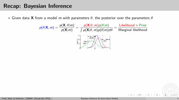
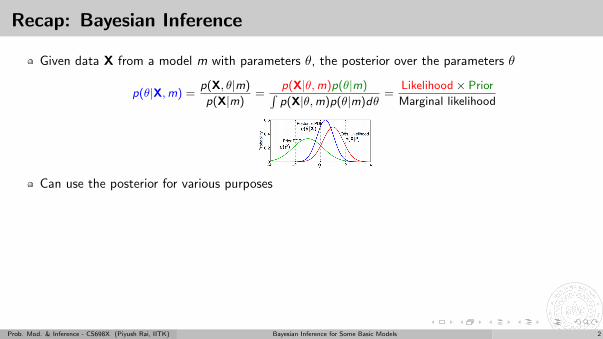
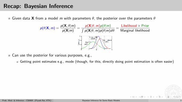
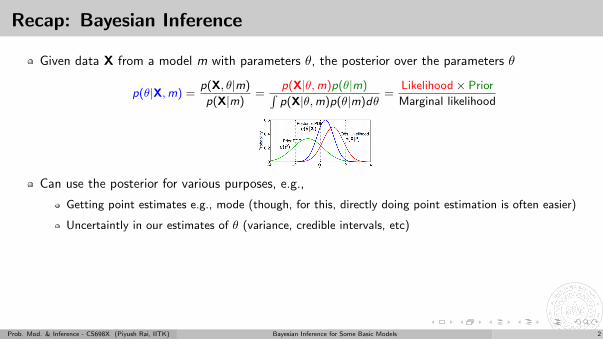
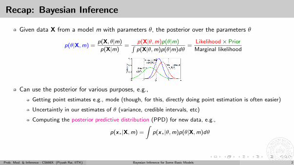
Given data X from a model m with parameters θ, the posterior over the parameters θ
p(θ|X,m) =p(X, θ|m)
p(X|m)
=p(X|θ,m)p(θ|m)∫p(X|θ,m)p(θ|m)dθ
=Likelihood× Prior
Marginal likelihood
Can use the posterior for various purposes, e.g.,
Getting point estimates e.g., mode (though, for this, directly doing point estimation is often easier)
Uncertaintly in our estimates of θ (variance, credible intervals, etc)
Computing the posterior predictive distribution (PPD) for new data, e.g.,
p(x∗|X,m) =
∫p(x∗|θ,m)p(θ|X,m)dθ
Caveat: Computing the posterior/PPD is in general hard (due to the intractable integrals involved)
Prob. Mod. & Inference - CS698X (Piyush Rai, IITK) Bayesian Inference for Some Basic Models 2
Recap: Bayesian Inference
Given data X from a model m with parameters θ, the posterior over the parameters θ
p(θ|X,m) =p(X, θ|m)
p(X|m)=
p(X|θ,m)p(θ|m)∫p(X|θ,m)p(θ|m)dθ
=Likelihood× Prior
Marginal likelihood
Can use the posterior for various purposes, e.g.,
Getting point estimates e.g., mode (though, for this, directly doing point estimation is often easier)
Uncertaintly in our estimates of θ (variance, credible intervals, etc)
Computing the posterior predictive distribution (PPD) for new data, e.g.,
p(x∗|X,m) =
∫p(x∗|θ,m)p(θ|X,m)dθ
Caveat: Computing the posterior/PPD is in general hard (due to the intractable integrals involved)
Prob. Mod. & Inference - CS698X (Piyush Rai, IITK) Bayesian Inference for Some Basic Models 2
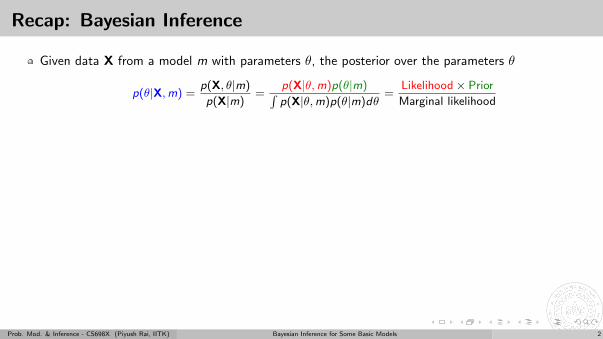
Recap: Bayesian Inference
Given data X from a model m with parameters θ, the posterior over the parameters θ
p(θ|X,m) =p(X, θ|m)
p(X|m)=
p(X|θ,m)p(θ|m)∫p(X|θ,m)p(θ|m)dθ
=Likelihood× Prior
Marginal likelihood
Can use the posterior for various purposes
, e.g.,
Getting point estimates e.g., mode (though, for this, directly doing point estimation is often easier)
Uncertaintly in our estimates of θ (variance, credible intervals, etc)
Computing the posterior predictive distribution (PPD) for new data, e.g.,
p(x∗|X,m) =
∫p(x∗|θ,m)p(θ|X,m)dθ
Caveat: Computing the posterior/PPD is in general hard (due to the intractable integrals involved)
Prob. Mod. & Inference - CS698X (Piyush Rai, IITK) Bayesian Inference for Some Basic Models 2
Recap: Bayesian Inference
Given data X from a model m with parameters θ, the posterior over the parameters θ
p(θ|X,m) =p(X, θ|m)
p(X|m)=
p(X|θ,m)p(θ|m)∫p(X|θ,m)p(θ|m)dθ
=Likelihood× Prior
Marginal likelihood
Can use the posterior for various purposes, e.g.,
Getting point estimates e.g., mode (though, for this, directly doing point estimation is often easier)
Uncertaintly in our estimates of θ (variance, credible intervals, etc)
Computing the posterior predictive distribution (PPD) for new data, e.g.,
p(x∗|X,m) =
∫p(x∗|θ,m)p(θ|X,m)dθ
Caveat: Computing the posterior/PPD is in general hard (due to the intractable integrals involved)
Prob. Mod. & Inference - CS698X (Piyush Rai, IITK) Bayesian Inference for Some Basic Models 2
Recap: Bayesian Inference
Given data X from a model m with parameters θ, the posterior over the parameters θ
p(θ|X,m) =p(X, θ|m)
p(X|m)=
p(X|θ,m)p(θ|m)∫p(X|θ,m)p(θ|m)dθ
=Likelihood× Prior
Marginal likelihood
Can use the posterior for various purposes, e.g.,
Getting point estimates e.g., mode (though, for this, directly doing point estimation is often easier)
Uncertaintly in our estimates of θ (variance, credible intervals, etc)
Computing the posterior predictive distribution (PPD) for new data, e.g.,
p(x∗|X,m) =
∫p(x∗|θ,m)p(θ|X,m)dθ
Caveat: Computing the posterior/PPD is in general hard (due to the intractable integrals involved)
Prob. Mod. & Inference - CS698X (Piyush Rai, IITK) Bayesian Inference for Some Basic Models 2
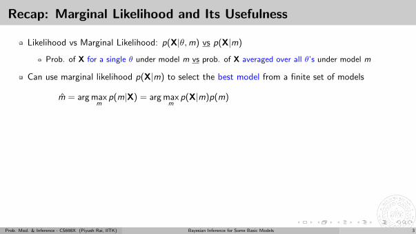
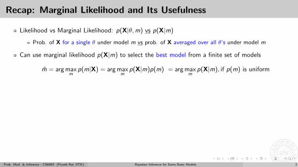
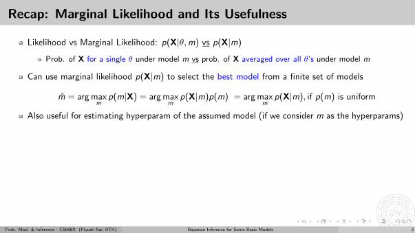
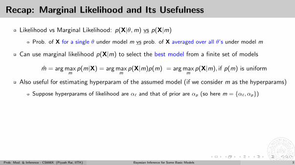
Recap: Marginal Likelihood and Its Usefulness
Likelihood vs Marginal Likelihood: p(X|θ,m) vs p(X|m)
Prob. of X for a single θ under model m vs prob. of X averaged over all θ’s under model m
Can use marginal likelihood p(X|m) to select the best model from a finite set of models
m̂ = arg maxm
p(m|X) = arg maxm
p(X|m)p(m) = arg maxm
p(X|m), if p(m) is uniform
Also useful for estimating hyperparam of the assumed model (if we consider m as the hyperparams)
Suppose hyperparams of likelihood are α` and that of prior are αp (so here m = {α`, αp})
Assuming p(α`, αp) is uniform, hyperparams can be estimated via MLE-II (a.k.a. empirical Bayes)
{α̂`, α̂p} = arg maxα`,αp
p(X|α`, αp) = arg maxα`,αp
∫p(X|θ, α`)p(θ|αp)dθ
Again, note that the integral here may be intractable and may need to be approximated
Can also compute p(m|X) and do Bayesian Model Averaging: p(x∗|X) =∑M
m=1 p(x∗|X,m)p(m|X)
Prob. Mod. & Inference - CS698X (Piyush Rai, IITK) Bayesian Inference for Some Basic Models 3
Recap: Marginal Likelihood and Its Usefulness
Likelihood vs Marginal Likelihood: p(X|θ,m) vs p(X|m)
Prob. of X for a single θ under model m vs prob. of X averaged over all θ’s under model m
Can use marginal likelihood p(X|m) to select the best model from a finite set of models
m̂ = arg maxm
p(m|X)
= arg maxm
p(X|m)p(m) = arg maxm
p(X|m), if p(m) is uniform
Also useful for estimating hyperparam of the assumed model (if we consider m as the hyperparams)
Suppose hyperparams of likelihood are α` and that of prior are αp (so here m = {α`, αp})
Assuming p(α`, αp) is uniform, hyperparams can be estimated via MLE-II (a.k.a. empirical Bayes)
{α̂`, α̂p} = arg maxα`,αp
p(X|α`, αp) = arg maxα`,αp
∫p(X|θ, α`)p(θ|αp)dθ
Again, note that the integral here may be intractable and may need to be approximated
Can also compute p(m|X) and do Bayesian Model Averaging: p(x∗|X) =∑M
m=1 p(x∗|X,m)p(m|X)
Prob. Mod. & Inference - CS698X (Piyush Rai, IITK) Bayesian Inference for Some Basic Models 3
Recap: Marginal Likelihood and Its Usefulness
Likelihood vs Marginal Likelihood: p(X|θ,m) vs p(X|m)
Prob. of X for a single θ under model m vs prob. of X averaged over all θ’s under model m
Can use marginal likelihood p(X|m) to select the best model from a finite set of models
m̂ = arg maxm
p(m|X) = arg maxm
p(X|m)p(m)
= arg maxm
p(X|m), if p(m) is uniform
Also useful for estimating hyperparam of the assumed model (if we consider m as the hyperparams)
Suppose hyperparams of likelihood are α` and that of prior are αp (so here m = {α`, αp})
Assuming p(α`, αp) is uniform, hyperparams can be estimated via MLE-II (a.k.a. empirical Bayes)
{α̂`, α̂p} = arg maxα`,αp
p(X|α`, αp) = arg maxα`,αp
∫p(X|θ, α`)p(θ|αp)dθ
Again, note that the integral here may be intractable and may need to be approximated
Can also compute p(m|X) and do Bayesian Model Averaging: p(x∗|X) =∑M
m=1 p(x∗|X,m)p(m|X)
Prob. Mod. & Inference - CS698X (Piyush Rai, IITK) Bayesian Inference for Some Basic Models 3
Recap: Marginal Likelihood and Its Usefulness
Likelihood vs Marginal Likelihood: p(X|θ,m) vs p(X|m)
Prob. of X for a single θ under model m vs prob. of X averaged over all θ’s under model m
Can use marginal likelihood p(X|m) to select the best model from a finite set of models
m̂ = arg maxm
p(m|X) = arg maxm
p(X|m)p(m) = arg maxm
p(X|m), if p(m) is uniform
Also useful for estimating hyperparam of the assumed model (if we consider m as the hyperparams)
Suppose hyperparams of likelihood are α` and that of prior are αp (so here m = {α`, αp})
Assuming p(α`, αp) is uniform, hyperparams can be estimated via MLE-II (a.k.a. empirical Bayes)
{α̂`, α̂p} = arg maxα`,αp
p(X|α`, αp) = arg maxα`,αp
∫p(X|θ, α`)p(θ|αp)dθ
Again, note that the integral here may be intractable and may need to be approximated
Can also compute p(m|X) and do Bayesian Model Averaging: p(x∗|X) =∑M
m=1 p(x∗|X,m)p(m|X)
Prob. Mod. & Inference - CS698X (Piyush Rai, IITK) Bayesian Inference for Some Basic Models 3
Recap: Marginal Likelihood and Its Usefulness
Likelihood vs Marginal Likelihood: p(X|θ,m) vs p(X|m)
Prob. of X for a single θ under model m vs prob. of X averaged over all θ’s under model m
Can use marginal likelihood p(X|m) to select the best model from a finite set of models
m̂ = arg maxm
p(m|X) = arg maxm
p(X|m)p(m) = arg maxm
p(X|m), if p(m) is uniform
Also useful for estimating hyperparam of the assumed model (if we consider m as the hyperparams)
Suppose hyperparams of likelihood are α` and that of prior are αp (so here m = {α`, αp})
Assuming p(α`, αp) is uniform, hyperparams can be estimated via MLE-II (a.k.a. empirical Bayes)
{α̂`, α̂p} = arg maxα`,αp
p(X|α`, αp)
= arg maxα`,αp
∫p(X|θ, α`)p(θ|αp)dθ
Again, note that the integral here may be intractable and may need to be approximated
Can also compute p(m|X) and do Bayesian Model Averaging: p(x∗|X) =∑M
m=1 p(x∗|X,m)p(m|X)
Prob. Mod. & Inference - CS698X (Piyush Rai, IITK) Bayesian Inference for Some Basic Models 3
Recap: Marginal Likelihood and Its Usefulness
Likelihood vs Marginal Likelihood: p(X|θ,m) vs p(X|m)
Prob. of X for a single θ under model m vs prob. of X averaged over all θ’s under model m
Can use marginal likelihood p(X|m) to select the best model from a finite set of models
m̂ = arg maxm
p(m|X) = arg maxm
p(X|m)p(m) = arg maxm
p(X|m), if p(m) is uniform
Also useful for estimating hyperparam of the assumed model (if we consider m as the hyperparams)
Suppose hyperparams of likelihood are α` and that of prior are αp (so here m = {α`, αp})
Assuming p(α`, αp) is uniform, hyperparams can be estimated via MLE-II (a.k.a. empirical Bayes)
{α̂`, α̂p} = arg maxα`,αp
p(X|α`, αp) = arg maxα`,αp
∫p(X|θ, α`)p(θ|αp)dθ
Again, note that the integral here may be intractable and may need to be approximated
Can also compute p(m|X) and do Bayesian Model Averaging: p(x∗|X) =∑M
m=1 p(x∗|X,m)p(m|X)
Prob. Mod. & Inference - CS698X (Piyush Rai, IITK) Bayesian Inference for Some Basic Models 3
Recap: Marginal Likelihood and Its Usefulness
Likelihood vs Marginal Likelihood: p(X|θ,m) vs p(X|m)
Prob. of X for a single θ under model m vs prob. of X averaged over all θ’s under model m
Can use marginal likelihood p(X|m) to select the best model from a finite set of models
m̂ = arg maxm
p(m|X) = arg maxm
p(X|m)p(m) = arg maxm
p(X|m), if p(m) is uniform
Also useful for estimating hyperparam of the assumed model (if we consider m as the hyperparams)
Suppose hyperparams of likelihood are α` and that of prior are αp (so here m = {α`, αp})
Assuming p(α`, αp) is uniform, hyperparams can be estimated via MLE-II (a.k.a. empirical Bayes)
{α̂`, α̂p} = arg maxα`,αp
p(X|α`, αp) = arg maxα`,αp
∫p(X|θ, α`)p(θ|αp)dθ
Again, note that the integral here may be intractable and may need to be approximated
Can also compute p(m|X) and do Bayesian Model Averaging: p(x∗|X) =∑M
m=1 p(x∗|X,m)p(m|X)
Prob. Mod. & Inference - CS698X (Piyush Rai, IITK) Bayesian Inference for Some Basic Models 3
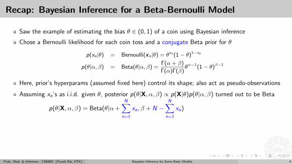
Recap: Bayesian Inference for a Beta-Bernoulli Model
Saw the example of estimating the bias θ ∈ (0, 1) of a coin using Bayesian inference
Chose a Bernoulli likelihood for each coin toss and a conjugate Beta prior for θ
p(xn|θ) = Bernoulli(xn|θ) = θxn (1− θ)1−xn
p(θ|α, β) = Beta(θ|α, β) =Γ(α + β)
Γ(α)Γ(β)θα−1(1− θ)β−1
Here, prior’s hyperparams (assumed fixed here) control its shape; also act as pseudo-observations
Assuming xn’s as i.i.d. given θ, posterior p(θ|X, α, β) ∝ p(X|θ)p(θ|α, β) turned out to be Beta
p(θ|X, α, β) = Beta(θ|α +N∑
n=1
xn, β + N −N∑
n=1
xn) = Beta(θ|α + N1, β + N0)
Note: Here posterior only depends on data X = {x1, . . . , xN} via sufficient statistics N1 and N0
p(θ|X, α, β) = p(θ|s(X))
We will see many other cases where the posterior depends on data only via some sufficient statistics
Prob. Mod. & Inference - CS698X (Piyush Rai, IITK) Bayesian Inference for Some Basic Models 4
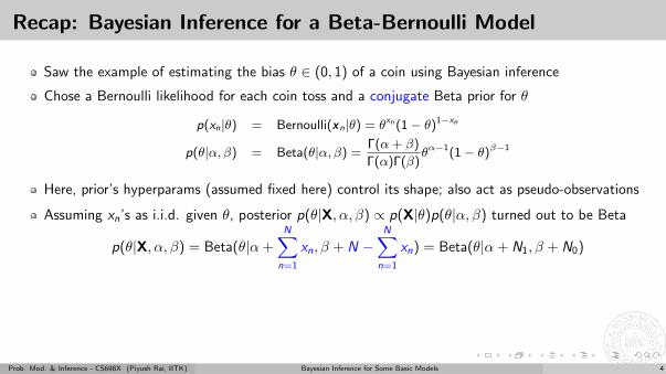
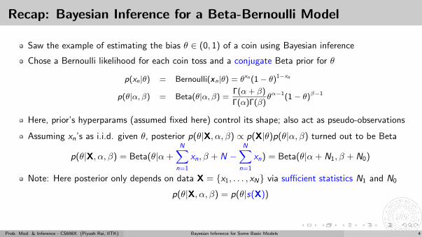
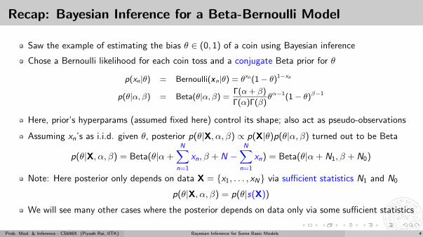
Recap: Bayesian Inference for a Beta-Bernoulli Model
Saw the example of estimating the bias θ ∈ (0, 1) of a coin using Bayesian inference
Chose a Bernoulli likelihood for each coin toss and a conjugate Beta prior for θ
p(xn|θ) = Bernoulli(xn|θ) = θxn (1− θ)1−xn
p(θ|α, β) = Beta(θ|α, β) =Γ(α + β)
Γ(α)Γ(β)θα−1(1− θ)β−1
Here, prior’s hyperparams (assumed fixed here) control its shape; also act as pseudo-observations
Assuming xn’s as i.i.d. given θ, posterior p(θ|X, α, β) ∝ p(X|θ)p(θ|α, β) turned out to be Beta
p(θ|X, α, β) = Beta(θ|α +N∑
n=1
xn, β + N −N∑
n=1
xn)
= Beta(θ|α + N1, β + N0)
Note: Here posterior only depends on data X = {x1, . . . , xN} via sufficient statistics N1 and N0
p(θ|X, α, β) = p(θ|s(X))
We will see many other cases where the posterior depends on data only via some sufficient statistics
Prob. Mod. & Inference - CS698X (Piyush Rai, IITK) Bayesian Inference for Some Basic Models 4
Recap: Bayesian Inference for a Beta-Bernoulli Model
Saw the example of estimating the bias θ ∈ (0, 1) of a coin using Bayesian inference
Chose a Bernoulli likelihood for each coin toss and a conjugate Beta prior for θ
p(xn|θ) = Bernoulli(xn|θ) = θxn (1− θ)1−xn
p(θ|α, β) = Beta(θ|α, β) =Γ(α + β)
Γ(α)Γ(β)θα−1(1− θ)β−1
Here, prior’s hyperparams (assumed fixed here) control its shape; also act as pseudo-observations
Assuming xn’s as i.i.d. given θ, posterior p(θ|X, α, β) ∝ p(X|θ)p(θ|α, β) turned out to be Beta
p(θ|X, α, β) = Beta(θ|α +N∑
n=1
xn, β + N −N∑
n=1
xn) = Beta(θ|α + N1, β + N0)
Note: Here posterior only depends on data X = {x1, . . . , xN} via sufficient statistics N1 and N0
p(θ|X, α, β) = p(θ|s(X))
We will see many other cases where the posterior depends on data only via some sufficient statistics
Prob. Mod. & Inference - CS698X (Piyush Rai, IITK) Bayesian Inference for Some Basic Models 4
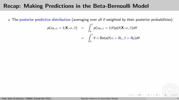
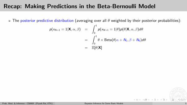
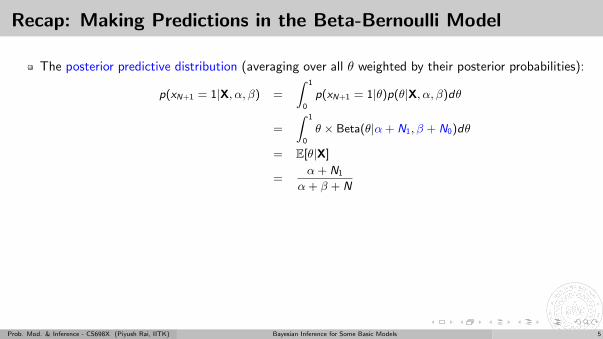
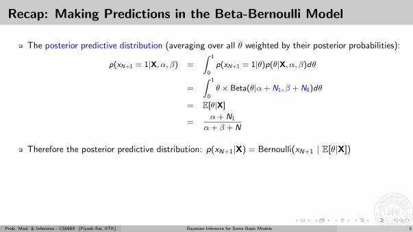
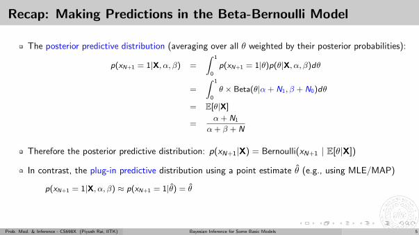
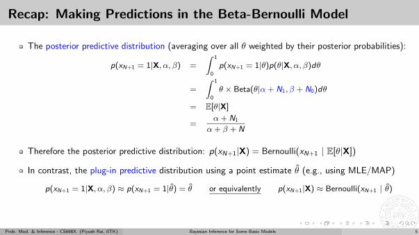
Recap: Making Predictions in the Beta-Bernoulli Model
The posterior predictive distribution (averaging over all θ weighted by their posterior probabilities):
p(xN+1 = 1|X, α, β) =
∫ 1
0
p(xN+1 = 1|θ)p(θ|X, α, β)dθ
=
∫ 1
0
θ × Beta(θ|α + N1, β + N0)dθ
= E[θ|X]
=α + N1
α + β + N
Therefore the posterior predictive distribution: p(xN+1|X) = Bernoulli(xN+1 | E[θ|X])
In contrast, the plug-in predictive distribution using a point estimate θ̂ (e.g., using MLE/MAP)
p(xN+1 = 1|X, α, β) ≈ p(xN+1 = 1|θ̂) = θ̂ or equivalently p(xN+1|X) ≈ Bernoulli(xN+1 | θ̂)
Prob. Mod. & Inference - CS698X (Piyush Rai, IITK) Bayesian Inference for Some Basic Models 5
Recap: Making Predictions in the Beta-Bernoulli Model
The posterior predictive distribution (averaging over all θ weighted by their posterior probabilities):
p(xN+1 = 1|X, α, β) =
∫ 1
0
p(xN+1 = 1|θ)p(θ|X, α, β)dθ
=
∫ 1
0
θ × Beta(θ|α + N1, β + N0)dθ
= E[θ|X]
=α + N1
α + β + N
Therefore the posterior predictive distribution: p(xN+1|X) = Bernoulli(xN+1 | E[θ|X])
In contrast, the plug-in predictive distribution using a point estimate θ̂ (e.g., using MLE/MAP)
p(xN+1 = 1|X, α, β) ≈ p(xN+1 = 1|θ̂) = θ̂
or equivalently p(xN+1|X) ≈ Bernoulli(xN+1 | θ̂)
Prob. Mod. & Inference - CS698X (Piyush Rai, IITK) Bayesian Inference for Some Basic Models 5
Recap: Making Predictions in the Beta-Bernoulli Model
The posterior predictive distribution (averaging over all θ weighted by their posterior probabilities):
p(xN+1 = 1|X, α, β) =
∫ 1
0
p(xN+1 = 1|θ)p(θ|X, α, β)dθ
=
∫ 1
0
θ × Beta(θ|α + N1, β + N0)dθ
= E[θ|X]
=α + N1
α + β + N
Therefore the posterior predictive distribution: p(xN+1|X) = Bernoulli(xN+1 | E[θ|X])
In contrast, the plug-in predictive distribution using a point estimate θ̂ (e.g., using MLE/MAP)
p(xN+1 = 1|X, α, β) ≈ p(xN+1 = 1|θ̂) = θ̂ or equivalently p(xN+1|X) ≈ Bernoulli(xN+1 | θ̂)
Prob. Mod. & Inference - CS698X (Piyush Rai, IITK) Bayesian Inference for Some Basic Models 5
More Examples..
Prob. Mod. & Inference - CS698X (Piyush Rai, IITK) Bayesian Inference for Some Basic Models 6
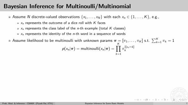
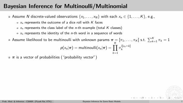
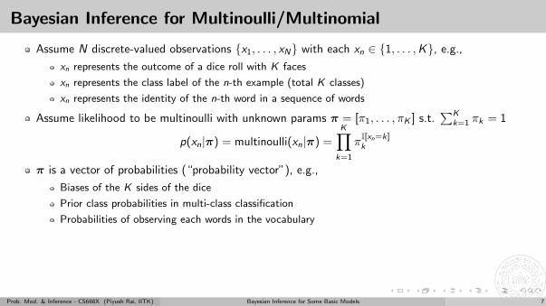
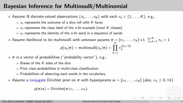
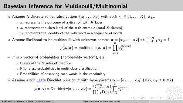
Bayesian Inference for Multinoulli/Multinomial
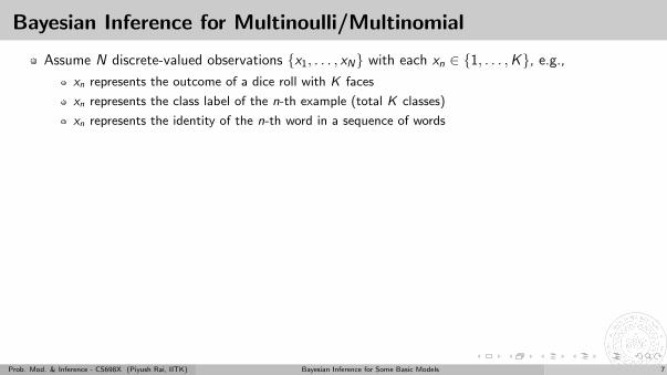
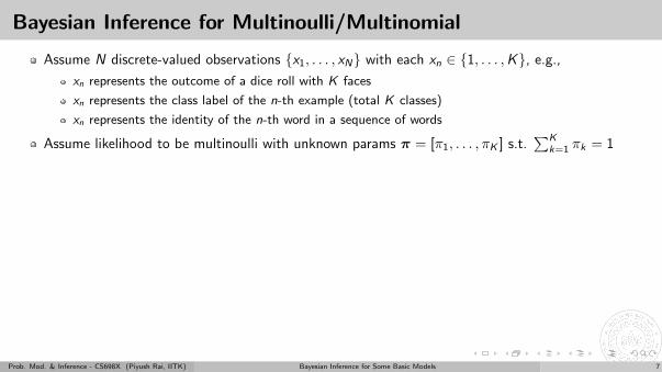
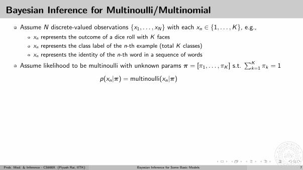
Assume N discrete-valued observations {x1, . . . , xN} with each xn ∈ {1, . . . ,K}
, e.g.,
xn represents the outcome of a dice roll with K faces
xn represents the class label of the n-th example (total K classes)
xn represents the identity of the n-th word in a sequence of words
Assume likelihood to be multinoulli with unknown params π = [π1, . . . , πK ] s.t.∑K
k=1 πk = 1
p(xn|π) = multinoulli(xn|π) =K∏
k=1
πI[xn=k]k
π is a vector of probabilities (“probability vector”), e.g.,
Biases of the K sides of the dice
Prior class probabilities in multi-class classification
Probabilities of observing each words in the vocabulary
Assume a conjugate Dirichlet prior on π with hyperparams α = [α1, . . . , αK ] (also, αk ≥ 0,∀k)
p(π|α) = Dirichlet(π|α1, . . . , αK ) =Γ(∑K
k=1 αk)∏Kk=1 Γ(αk)
K∏k=1
παk−1k =
1
B(α)
K∏k=1
παk−1k
Prob. Mod. & Inference - CS698X (Piyush Rai, IITK) Bayesian Inference for Some Basic Models 7
Bayesian Inference for Multinoulli/Multinomial
Assume N discrete-valued observations {x1, . . . , xN} with each xn ∈ {1, . . . ,K}, e.g.,
xn represents the outcome of a dice roll with K faces
xn represents the class label of the n-th example (total K classes)
xn represents the identity of the n-th word in a sequence of words
Assume likelihood to be multinoulli with unknown params π = [π1, . . . , πK ] s.t.∑K
k=1 πk = 1
p(xn|π) = multinoulli(xn|π)
=K∏
k=1
πI[xn=k]k
π is a vector of probabilities (“probability vector”), e.g.,
Biases of the K sides of the dice
Prior class probabilities in multi-class classification
Probabilities of observing each words in the vocabulary
Assume a conjugate Dirichlet prior on π with hyperparams α = [α1, . . . , αK ] (also, αk ≥ 0,∀k)
p(π|α) = Dirichlet(π|α1, . . . , αK ) =Γ(∑K
k=1 αk)∏Kk=1 Γ(αk)
K∏k=1
παk−1k =
1
B(α)
K∏k=1
παk−1k
Prob. Mod. & Inference - CS698X (Piyush Rai, IITK) Bayesian Inference for Some Basic Models 7
Bayesian Inference for Multinoulli/Multinomial
Assume N discrete-valued observations {x1, . . . , xN} with each xn ∈ {1, . . . ,K}, e.g.,
xn represents the outcome of a dice roll with K faces
xn represents the class label of the n-th example (total K classes)
xn represents the identity of the n-th word in a sequence of words
Assume likelihood to be multinoulli with unknown params π = [π1, . . . , πK ] s.t.∑K
k=1 πk = 1
p(xn|π) = multinoulli(xn|π) =K∏
k=1
πI[xn=k]k
π is a vector of probabilities (“probability vector”), e.g.,
Biases of the K sides of the dice
Prior class probabilities in multi-class classification
Probabilities of observing each words in the vocabulary
Assume a conjugate Dirichlet prior on π with hyperparams α = [α1, . . . , αK ] (also, αk ≥ 0,∀k)
p(π|α) = Dirichlet(π|α1, . . . , αK ) =Γ(∑K
k=1 αk)∏Kk=1 Γ(αk)
K∏k=1
παk−1k =
1
B(α)
K∏k=1
παk−1k
Prob. Mod. & Inference - CS698X (Piyush Rai, IITK) Bayesian Inference for Some Basic Models 7
Bayesian Inference for Multinoulli/Multinomial
Assume N discrete-valued observations {x1, . . . , xN} with each xn ∈ {1, . . . ,K}, e.g.,
xn represents the outcome of a dice roll with K faces
xn represents the class label of the n-th example (total K classes)
xn represents the identity of the n-th word in a sequence of words
Assume likelihood to be multinoulli with unknown params π = [π1, . . . , πK ] s.t.∑K
k=1 πk = 1
p(xn|π) = multinoulli(xn|π) =K∏
k=1
πI[xn=k]k
π is a vector of probabilities (“probability vector”)
, e.g.,
Biases of the K sides of the dice
Prior class probabilities in multi-class classification
Probabilities of observing each words in the vocabulary
Assume a conjugate Dirichlet prior on π with hyperparams α = [α1, . . . , αK ] (also, αk ≥ 0,∀k)
p(π|α) = Dirichlet(π|α1, . . . , αK ) =Γ(∑K
k=1 αk)∏Kk=1 Γ(αk)
K∏k=1
παk−1k =
1
B(α)
K∏k=1
παk−1k
Prob. Mod. & Inference - CS698X (Piyush Rai, IITK) Bayesian Inference for Some Basic Models 7
Bayesian Inference for Multinoulli/Multinomial
Assume N discrete-valued observations {x1, . . . , xN} with each xn ∈ {1, . . . ,K}, e.g.,
xn represents the outcome of a dice roll with K faces
xn represents the class label of the n-th example (total K classes)
xn represents the identity of the n-th word in a sequence of words
Assume likelihood to be multinoulli with unknown params π = [π1, . . . , πK ] s.t.∑K
k=1 πk = 1
p(xn|π) = multinoulli(xn|π) =K∏
k=1
πI[xn=k]k
π is a vector of probabilities (“probability vector”), e.g.,
Biases of the K sides of the dice
Prior class probabilities in multi-class classification
Probabilities of observing each words in the vocabulary
Assume a conjugate Dirichlet prior on π with hyperparams α = [α1, . . . , αK ] (also, αk ≥ 0,∀k)
p(π|α) = Dirichlet(π|α1, . . . , αK ) =Γ(∑K
k=1 αk)∏Kk=1 Γ(αk)
K∏k=1
παk−1k =
1
B(α)
K∏k=1
παk−1k
Prob. Mod. & Inference - CS698X (Piyush Rai, IITK) Bayesian Inference for Some Basic Models 7
Bayesian Inference for Multinoulli/Multinomial
Assume N discrete-valued observations {x1, . . . , xN} with each xn ∈ {1, . . . ,K}, e.g.,
xn represents the outcome of a dice roll with K faces
xn represents the class label of the n-th example (total K classes)
xn represents the identity of the n-th word in a sequence of words
Assume likelihood to be multinoulli with unknown params π = [π1, . . . , πK ] s.t.∑K
k=1 πk = 1
p(xn|π) = multinoulli(xn|π) =K∏
k=1
πI[xn=k]k
π is a vector of probabilities (“probability vector”), e.g.,
Biases of the K sides of the dice
Prior class probabilities in multi-class classification
Probabilities of observing each words in the vocabulary
Assume a conjugate Dirichlet prior on π with hyperparams α = [α1, . . . , αK ] (also, αk ≥ 0,∀k)
p(π|α) = Dirichlet(π|α1, . . . , αK )
=Γ(∑K
k=1 αk)∏Kk=1 Γ(αk)
K∏k=1
παk−1k =
1
B(α)
K∏k=1
παk−1k
Prob. Mod. & Inference - CS698X (Piyush Rai, IITK) Bayesian Inference for Some Basic Models 7
Bayesian Inference for Multinoulli/Multinomial
Assume N discrete-valued observations {x1, . . . , xN} with each xn ∈ {1, . . . ,K}, e.g.,
xn represents the outcome of a dice roll with K faces
xn represents the class label of the n-th example (total K classes)
xn represents the identity of the n-th word in a sequence of words
Assume likelihood to be multinoulli with unknown params π = [π1, . . . , πK ] s.t.∑K
k=1 πk = 1
p(xn|π) = multinoulli(xn|π) =K∏
k=1
πI[xn=k]k
π is a vector of probabilities (“probability vector”), e.g.,
Biases of the K sides of the dice
Prior class probabilities in multi-class classification
Probabilities of observing each words in the vocabulary
Assume a conjugate Dirichlet prior on π with hyperparams α = [α1, . . . , αK ] (also, αk ≥ 0,∀k)
p(π|α) = Dirichlet(π|α1, . . . , αK ) =Γ(∑K
k=1 αk)∏Kk=1 Γ(αk)
K∏k=1
παk−1k
=1
B(α)
K∏k=1
παk−1k
Prob. Mod. & Inference - CS698X (Piyush Rai, IITK) Bayesian Inference for Some Basic Models 7
Bayesian Inference for Multinoulli/Multinomial
Assume N discrete-valued observations {x1, . . . , xN} with each xn ∈ {1, . . . ,K}, e.g.,
xn represents the outcome of a dice roll with K faces
xn represents the class label of the n-th example (total K classes)
xn represents the identity of the n-th word in a sequence of words
Assume likelihood to be multinoulli with unknown params π = [π1, . . . , πK ] s.t.∑K
k=1 πk = 1
p(xn|π) = multinoulli(xn|π) =K∏
k=1
πI[xn=k]k
π is a vector of probabilities (“probability vector”), e.g.,
Biases of the K sides of the dice
Prior class probabilities in multi-class classification
Probabilities of observing each words in the vocabulary
Assume a conjugate Dirichlet prior on π with hyperparams α = [α1, . . . , αK ] (also, αk ≥ 0,∀k)
p(π|α) = Dirichlet(π|α1, . . . , αK ) =Γ(∑K
k=1 αk)∏Kk=1 Γ(αk)
K∏k=1
παk−1k =
1
B(α)
K∏k=1
παk−1k
Prob. Mod. & Inference - CS698X (Piyush Rai, IITK) Bayesian Inference for Some Basic Models 7
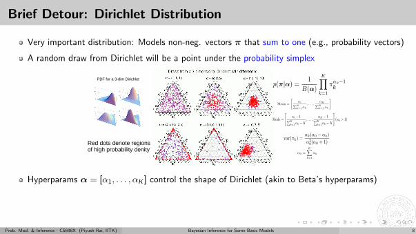
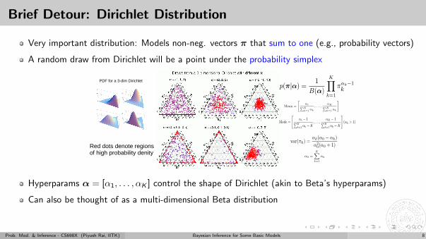
Brief Detour: Dirichlet Distribution
Very important distribution: Models non-neg. vectors π that sum to one (e.g., probability vectors)
A random draw from Dirichlet will be a point under the probability simplex
Red dots denote regions of high probability denity
PDF for a 3-dim Dirichlet
Hyperparams α = [α1, . . . , αK ] control the shape of Dirichlet (akin to Beta’s hyperparams)
Can also be thought of as a multi-dimensional Beta distribution
Note: Can also be seen as normalized version of K independent gamma random variables
Prob. Mod. & Inference - CS698X (Piyush Rai, IITK) Bayesian Inference for Some Basic Models 8
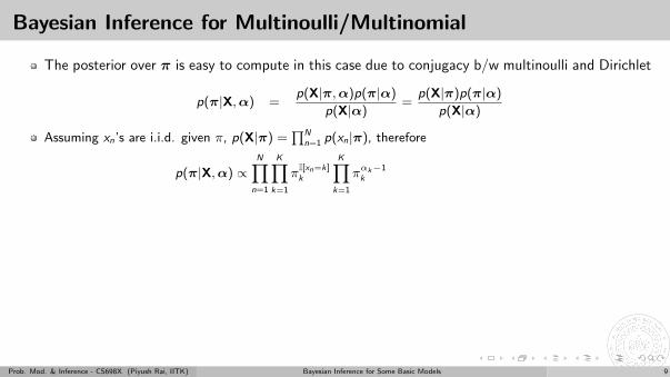
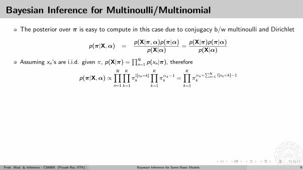
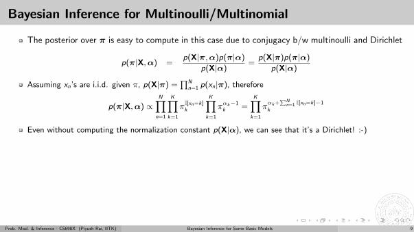
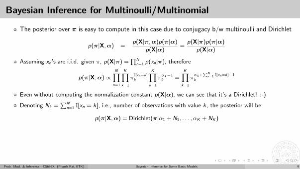
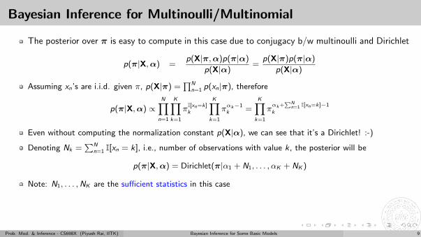
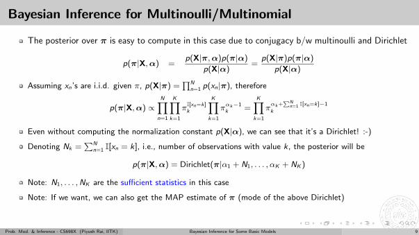
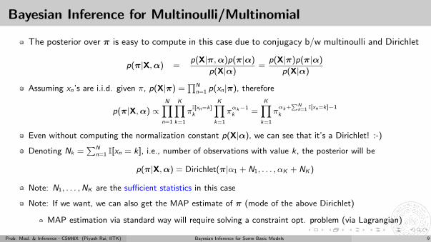
Bayesian Inference for Multinoulli/Multinomial
The posterior over π is easy to compute in this case due to conjugacy b/w multinoulli and Dirichlet
p(π|X,α) =p(X|π,α)p(π|α)
p(X|α)=
p(X|π)p(π|α)
p(X|α)
Assuming xn’s are i.i.d. given π, p(X|π) =∏N
n=1 p(xn|π), therefore
p(π|X,α) ∝N∏
n=1
K∏k=1
πI[xn=k]k
K∏k=1
παk−1k =
K∏k=1
παk+
∑Nn=1 I[xn=k]−1
k
Even without computing the normalization constant p(X|α), we can see that it’s a Dirichlet! :-)
Denoting Nk =∑N
n=1 I[xn = k], i.e., number of observations with value k, the posterior will be
p(π|X,α) = Dirichlet(π|α1 + N1, . . . , αK + NK )
Note: N1, . . . ,NK are the sufficient statistics in this case
Note: If we want, we can also get the MAP estimate of π (mode of the above Dirichlet)
MAP estimation via standard way will require solving a constraint opt. problem (via Lagrangian)
Prob. Mod. & Inference - CS698X (Piyush Rai, IITK) Bayesian Inference for Some Basic Models 9
Bayesian Inference for Multinoulli/Multinomial
The posterior over π is easy to compute in this case due to conjugacy b/w multinoulli and Dirichlet
p(π|X,α) =p(X|π,α)p(π|α)
p(X|α)=
p(X|π)p(π|α)
p(X|α)
Assuming xn’s are i.i.d. given π, p(X|π) =∏N
n=1 p(xn|π), therefore
p(π|X,α) ∝N∏
n=1
K∏k=1
πI[xn=k]k
K∏k=1
παk−1k
=K∏
k=1
παk+
∑Nn=1 I[xn=k]−1
k
Even without computing the normalization constant p(X|α), we can see that it’s a Dirichlet! :-)
Denoting Nk =∑N
n=1 I[xn = k], i.e., number of observations with value k, the posterior will be
p(π|X,α) = Dirichlet(π|α1 + N1, . . . , αK + NK )
Note: N1, . . . ,NK are the sufficient statistics in this case
Note: If we want, we can also get the MAP estimate of π (mode of the above Dirichlet)
MAP estimation via standard way will require solving a constraint opt. problem (via Lagrangian)
Prob. Mod. & Inference - CS698X (Piyush Rai, IITK) Bayesian Inference for Some Basic Models 9
Bayesian Inference for Multinoulli/Multinomial
The posterior over π is easy to compute in this case due to conjugacy b/w multinoulli and Dirichlet
p(π|X,α) =p(X|π,α)p(π|α)
p(X|α)=
p(X|π)p(π|α)
p(X|α)
Assuming xn’s are i.i.d. given π, p(X|π) =∏N
n=1 p(xn|π), therefore
p(π|X,α) ∝N∏
n=1
K∏k=1
πI[xn=k]k
K∏k=1
παk−1k =
K∏k=1
παk+
∑Nn=1 I[xn=k]−1
k
Even without computing the normalization constant p(X|α), we can see that it’s a Dirichlet! :-)
Denoting Nk =∑N
n=1 I[xn = k], i.e., number of observations with value k, the posterior will be
p(π|X,α) = Dirichlet(π|α1 + N1, . . . , αK + NK )
Note: N1, . . . ,NK are the sufficient statistics in this case
Note: If we want, we can also get the MAP estimate of π (mode of the above Dirichlet)
MAP estimation via standard way will require solving a constraint opt. problem (via Lagrangian)
Prob. Mod. & Inference - CS698X (Piyush Rai, IITK) Bayesian Inference for Some Basic Models 9
Bayesian Inference for Multinoulli/Multinomial
The posterior over π is easy to compute in this case due to conjugacy b/w multinoulli and Dirichlet
p(π|X,α) =p(X|π,α)p(π|α)
p(X|α)=
p(X|π)p(π|α)
p(X|α)
Assuming xn’s are i.i.d. given π, p(X|π) =∏N
n=1 p(xn|π), therefore
p(π|X,α) ∝N∏
n=1
K∏k=1
πI[xn=k]k
K∏k=1
παk−1k =
K∏k=1
παk+
∑Nn=1 I[xn=k]−1
k
Even without computing the normalization constant p(X|α), we can see that it’s a Dirichlet! :-)
Denoting Nk =∑N
n=1 I[xn = k], i.e., number of observations with value k, the posterior will be
p(π|X,α) = Dirichlet(π|α1 + N1, . . . , αK + NK )
Note: N1, . . . ,NK are the sufficient statistics in this case
Note: If we want, we can also get the MAP estimate of π (mode of the above Dirichlet)
MAP estimation via standard way will require solving a constraint opt. problem (via Lagrangian)
Prob. Mod. & Inference - CS698X (Piyush Rai, IITK) Bayesian Inference for Some Basic Models 9
Bayesian Inference for Multinoulli/Multinomial
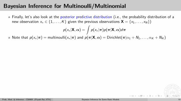
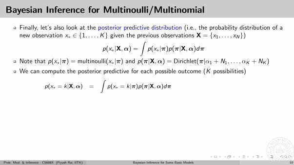
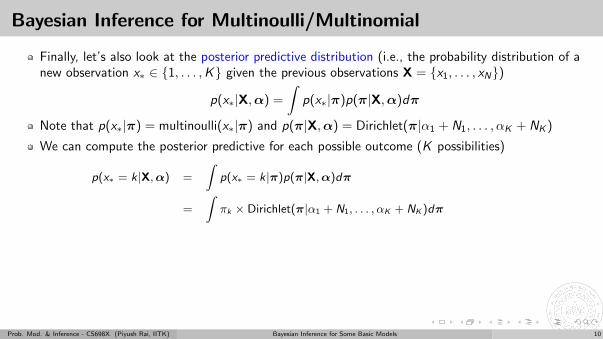
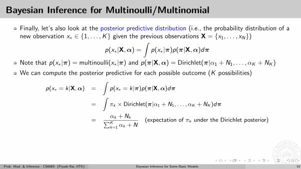
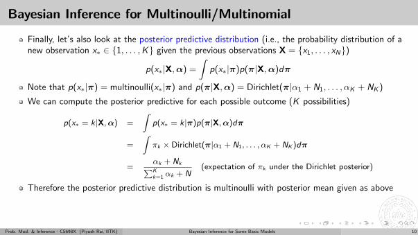
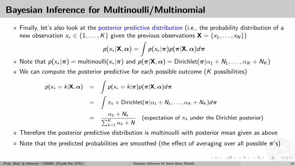
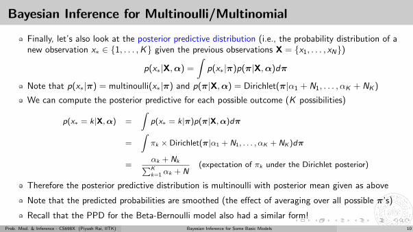
Finally, let’s also look at the posterior predictive distribution (i.e., the probability distribution of anew observation x∗ ∈ {1, . . . ,K} given the previous observations X = {x1, . . . , xN})
p(x∗|X,α) =
∫p(x∗|π)p(π|X,α)dπ
Note that p(x∗|π) = multinoulli(x∗|π) and p(π|X,α) = Dirichlet(π|α1 + N1, . . . , αK + NK )
We can compute the posterior predictive for each possible outcome (K possibilities)
p(x∗ = k|X,α) =
∫p(x∗ = k|π)p(π|X,α)dπ
=
∫πk × Dirichlet(π|α1 + N1, . . . , αK + NK )dπ
=αk + Nk∑Kk=1 αk + N
(expectation of πk under the Dirichlet posterior)
Therefore the posterior predictive distribution is multinoulli with posterior mean given as above
Note that the predicted probabilities are smoothed (the effect of averaging over all possible π’s)
Recall that the PPD for the Beta-Bernoulli model also had a similar form!
Prob. Mod. & Inference - CS698X (Piyush Rai, IITK) Bayesian Inference for Some Basic Models 10
Bayesian Inference for Multinoulli/Multinomial
Finally, let’s also look at the posterior predictive distribution (i.e., the probability distribution of anew observation x∗ ∈ {1, . . . ,K} given the previous observations X = {x1, . . . , xN})
p(x∗|X,α) =
∫p(x∗|π)p(π|X,α)dπ
Note that p(x∗|π) = multinoulli(x∗|π) and p(π|X,α) = Dirichlet(π|α1 + N1, . . . , αK + NK )
We can compute the posterior predictive for each possible outcome (K possibilities)
p(x∗ = k|X,α) =
∫p(x∗ = k|π)p(π|X,α)dπ
=
∫πk × Dirichlet(π|α1 + N1, . . . , αK + NK )dπ
=αk + Nk∑Kk=1 αk + N
(expectation of πk under the Dirichlet posterior)
Therefore the posterior predictive distribution is multinoulli with posterior mean given as above
Note that the predicted probabilities are smoothed (the effect of averaging over all possible π’s)
Recall that the PPD for the Beta-Bernoulli model also had a similar form!
Prob. Mod. & Inference - CS698X (Piyush Rai, IITK) Bayesian Inference for Some Basic Models 10
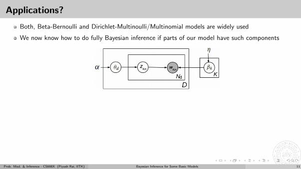
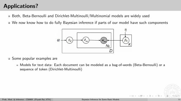
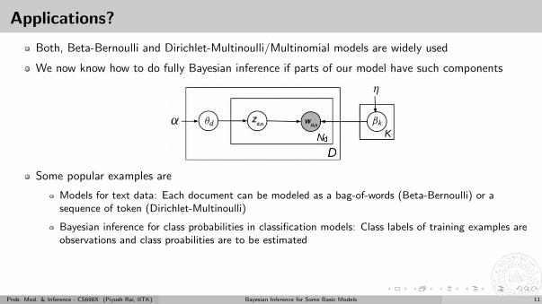
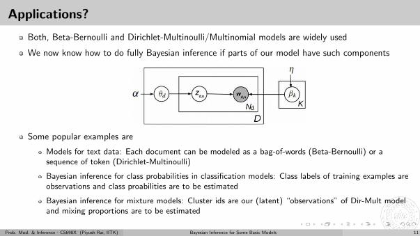
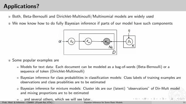
Applications?
Both, Beta-Bernoulli and Dirichlet-Multinoulli/Multinomial models are widely used
We now know how to do fully Bayesian inference if parts of our model have such components
Some popular examples are
Models for text data: Each document can be modeled as a bag-of-words (Beta-Bernoulli) or asequence of token (Dirichlet-Multinoulli)
Bayesian inference for class probabilities in classification models: Class labels of training examples areobservations and class proabilities are to be estimated
Bayesian inference for mixture models: Cluster ids are our (latent) “observations” of Dir-Mult modeland mixing proportions are to be estimated
.. and several others, which we will see later..
Prob. Mod. & Inference - CS698X (Piyush Rai, IITK) Bayesian Inference for Some Basic Models 11
Applications?
Both, Beta-Bernoulli and Dirichlet-Multinoulli/Multinomial models are widely used
We now know how to do fully Bayesian inference if parts of our model have such components
Some popular examples are
Models for text data: Each document can be modeled as a bag-of-words (Beta-Bernoulli) or asequence of token (Dirichlet-Multinoulli)
Bayesian inference for class probabilities in classification models: Class labels of training examples areobservations and class proabilities are to be estimated
Bayesian inference for mixture models: Cluster ids are our (latent) “observations” of Dir-Mult modeland mixing proportions are to be estimated
.. and several others, which we will see later..Prob. Mod. & Inference - CS698X (Piyush Rai, IITK) Bayesian Inference for Some Basic Models 11
Some More Examples..
Prob. Mod. & Inference - CS698X (Piyush Rai, IITK) Bayesian Inference for Some Basic Models 12
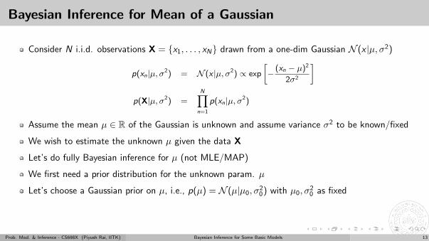
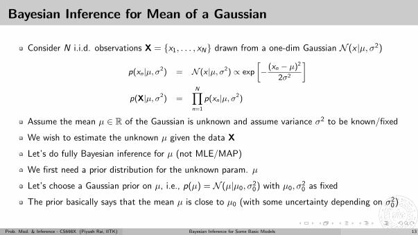
Bayesian Inference for Mean of a Gaussian
Consider N i.i.d. observations X = {x1, . . . , xN} drawn from a one-dim Gaussian N (x |µ, σ2)
p(xn|µ, σ2) = N (x |µ, σ2) ∝ exp
[− (xn − µ)2
2σ2
]p(X|µ, σ2) =
N∏n=1
p(xn|µ, σ2)
Assume the mean µ ∈ R of the Gaussian is unknown and assume variance σ2 to be known/fixed
We wish to estimate the unknown µ given the data X
Let’s do fully Bayesian inference for µ (not MLE/MAP)
We first need a prior distribution for the unknown param. µ
Let’s choose a Gaussian prior on µ, i.e., p(µ) = N (µ|µ0, σ20) with µ0, σ
20 as fixed
The prior basically says that the mean µ is close to µ0 (with some uncertainty depending on σ20)
Prob. Mod. & Inference - CS698X (Piyush Rai, IITK) Bayesian Inference for Some Basic Models 13
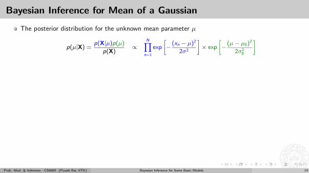
Bayesian Inference for Mean of a Gaussian
The posterior distribution for the unknown mean parameter µ
p(µ|X) =p(X|µ)p(µ)
p(X)∝
N∏n=1
exp
[− (xn − µ)2
2σ2
]× exp
[− (µ− µ0)2
2σ20
]
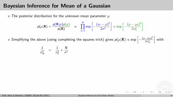
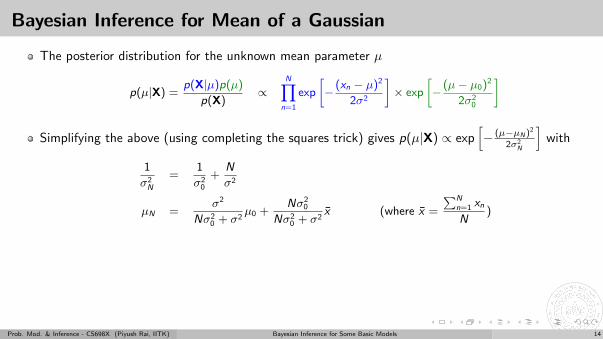
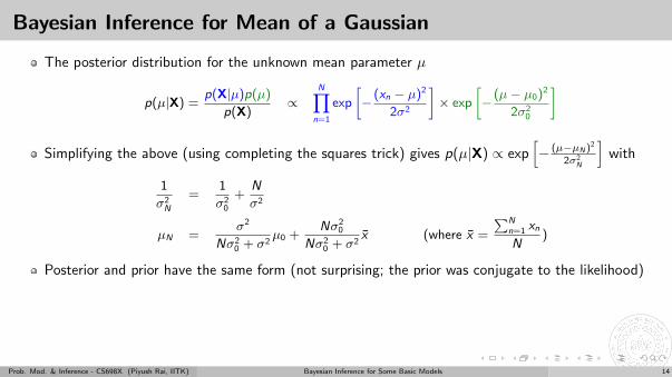
Simplifying the above (using completing the squares trick) gives p(µ|X) ∝ exp[− (µ−µN )2
2σ2N
]with
1
σ2N
=1
σ20
+N
σ2
µN =σ2
Nσ20 + σ2
µ0 +Nσ2
0
Nσ20 + σ2
x̄ (where x̄ =
∑Nn=1 xn
N)
Posterior and prior have the same form (not surprising; the prior was conjugate to the likelihood)
Consider what happens as N (number of observations) grows very large?
The posterior’s variance σ2N approaches σ2/N (and goes to 0 as N →∞)
The posterior’s mean µN approaches x̄ (which is also the MLE solution)
Prob. Mod. & Inference - CS698X (Piyush Rai, IITK) Bayesian Inference for Some Basic Models 14
Bayesian Inference for Mean of a Gaussian
The posterior distribution for the unknown mean parameter µ
p(µ|X) =p(X|µ)p(µ)
p(X)∝
N∏n=1
exp
[− (xn − µ)2
2σ2
]× exp
[− (µ− µ0)2
2σ20
]
Simplifying the above (using completing the squares trick) gives p(µ|X) ∝ exp[− (µ−µN )2
2σ2N
]with
1
σ2N
=1
σ20
+N
σ2
µN =σ2
Nσ20 + σ2
µ0 +Nσ2
0
Nσ20 + σ2
x̄ (where x̄ =
∑Nn=1 xn
N)
Posterior and prior have the same form (not surprising; the prior was conjugate to the likelihood)
Consider what happens as N (number of observations) grows very large?
The posterior’s variance σ2N approaches σ2/N (and goes to 0 as N →∞)
The posterior’s mean µN approaches x̄ (which is also the MLE solution)
Prob. Mod. & Inference - CS698X (Piyush Rai, IITK) Bayesian Inference for Some Basic Models 14
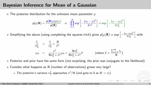
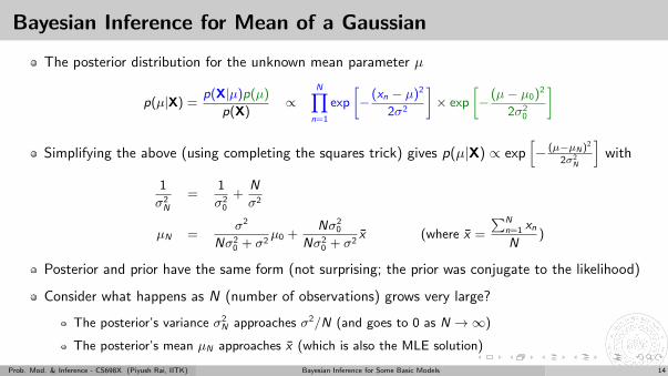
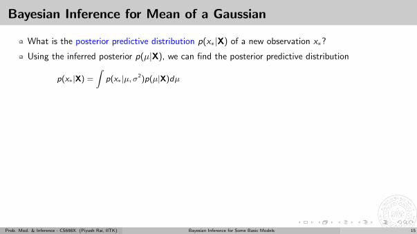
Bayesian Inference for Mean of a Gaussian
What is the posterior predictive distribution p(x∗|X) of a new observation x∗?
Using the inferred posterior p(µ|X), we can find the posterior predictive distribution
p(x∗|X) =
∫p(x∗|µ, σ2)p(µ|X)dµ
=
∫N (x∗|µ, σ2)N (µ|µN , σ
2N)dµ = N (x∗|µN , σ
2 + σ2N)
Note; Can also get the above result by thinking of x∗ as x∗ = µ+ ε where µ ∼ N (µN , σ2N), and
ε ∼ N (0, σ2) is independently added observation noise
Note that, as per the above, the uncertainty in distribution of x∗ now has two components
σ2: Due to the noisy observation model, σ2N : Due to the uncertainty in µ
In contrast, the plug-in predictive posterior, given a point estimate µ̂ (e.g., MLE/MAP) would be
p(x∗|X) =
∫p(x∗|µ, σ2)p(µ|X)dµ ≈ p(x∗|µ̂, σ2) = N (x∗|µ̂, σ2)
.. which doesn’t incorporate the uncertainty in our estimate of µ (since we used a point estimate)
Note that as N →∞, both approaches would give the same p(x∗|X) since σ2N → 0
Prob. Mod. & Inference - CS698X (Piyush Rai, IITK) Bayesian Inference for Some Basic Models 15
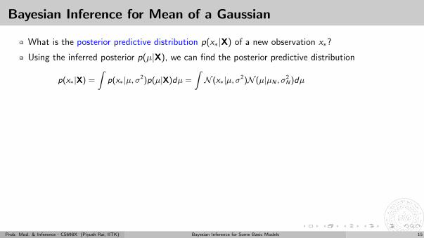
Bayesian Inference for Mean of a Gaussian
What is the posterior predictive distribution p(x∗|X) of a new observation x∗?
Using the inferred posterior p(µ|X), we can find the posterior predictive distribution
p(x∗|X) =
∫p(x∗|µ, σ2)p(µ|X)dµ =
∫N (x∗|µ, σ2)N (µ|µN , σ
2N)dµ
= N (x∗|µN , σ2 + σ2
N)
Note; Can also get the above result by thinking of x∗ as x∗ = µ+ ε where µ ∼ N (µN , σ2N), and
ε ∼ N (0, σ2) is independently added observation noise
Note that, as per the above, the uncertainty in distribution of x∗ now has two components
σ2: Due to the noisy observation model, σ2N : Due to the uncertainty in µ
In contrast, the plug-in predictive posterior, given a point estimate µ̂ (e.g., MLE/MAP) would be
p(x∗|X) =
∫p(x∗|µ, σ2)p(µ|X)dµ ≈ p(x∗|µ̂, σ2) = N (x∗|µ̂, σ2)
.. which doesn’t incorporate the uncertainty in our estimate of µ (since we used a point estimate)
Note that as N →∞, both approaches would give the same p(x∗|X) since σ2N → 0
Prob. Mod. & Inference - CS698X (Piyush Rai, IITK) Bayesian Inference for Some Basic Models 15
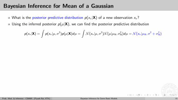
Bayesian Inference for Mean of a Gaussian
What is the posterior predictive distribution p(x∗|X) of a new observation x∗?
Using the inferred posterior p(µ|X), we can find the posterior predictive distribution
p(x∗|X) =
∫p(x∗|µ, σ2)p(µ|X)dµ =
∫N (x∗|µ, σ2)N (µ|µN , σ
2N)dµ = N (x∗|µN , σ
2 + σ2N)
Note; Can also get the above result by thinking of x∗ as x∗ = µ+ ε where µ ∼ N (µN , σ2N), and
ε ∼ N (0, σ2) is independently added observation noise
Note that, as per the above, the uncertainty in distribution of x∗ now has two components
σ2: Due to the noisy observation model, σ2N : Due to the uncertainty in µ
In contrast, the plug-in predictive posterior, given a point estimate µ̂ (e.g., MLE/MAP) would be
p(x∗|X) =
∫p(x∗|µ, σ2)p(µ|X)dµ ≈ p(x∗|µ̂, σ2) = N (x∗|µ̂, σ2)
.. which doesn’t incorporate the uncertainty in our estimate of µ (since we used a point estimate)
Note that as N →∞, both approaches would give the same p(x∗|X) since σ2N → 0
Prob. Mod. & Inference - CS698X (Piyush Rai, IITK) Bayesian Inference for Some Basic Models 15
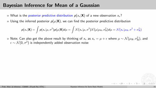
Bayesian Inference for Mean of a Gaussian
What is the posterior predictive distribution p(x∗|X) of a new observation x∗?
Using the inferred posterior p(µ|X), we can find the posterior predictive distribution
p(x∗|X) =
∫p(x∗|µ, σ2)p(µ|X)dµ =
∫N (x∗|µ, σ2)N (µ|µN , σ
2N)dµ = N (x∗|µN , σ
2 + σ2N)
Note; Can also get the above result by thinking of x∗ as x∗ = µ+ ε where µ ∼ N (µN , σ2N), and
ε ∼ N (0, σ2) is independently added observation noise
Note that, as per the above, the uncertainty in distribution of x∗ now has two components
σ2: Due to the noisy observation model, σ2N : Due to the uncertainty in µ
In contrast, the plug-in predictive posterior, given a point estimate µ̂ (e.g., MLE/MAP) would be
p(x∗|X) =
∫p(x∗|µ, σ2)p(µ|X)dµ ≈ p(x∗|µ̂, σ2) = N (x∗|µ̂, σ2)
.. which doesn’t incorporate the uncertainty in our estimate of µ (since we used a point estimate)
Note that as N →∞, both approaches would give the same p(x∗|X) since σ2N → 0
Prob. Mod. & Inference - CS698X (Piyush Rai, IITK) Bayesian Inference for Some Basic Models 15
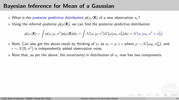
Bayesian Inference for Mean of a Gaussian
What is the posterior predictive distribution p(x∗|X) of a new observation x∗?
Using the inferred posterior p(µ|X), we can find the posterior predictive distribution
p(x∗|X) =
∫p(x∗|µ, σ2)p(µ|X)dµ =
∫N (x∗|µ, σ2)N (µ|µN , σ
2N)dµ = N (x∗|µN , σ
2 + σ2N)
Note; Can also get the above result by thinking of x∗ as x∗ = µ+ ε where µ ∼ N (µN , σ2N), and
ε ∼ N (0, σ2) is independently added observation noise
Note that, as per the above, the uncertainty in distribution of x∗ now has two components
σ2: Due to the noisy observation model, σ2N : Due to the uncertainty in µ
In contrast, the plug-in predictive posterior, given a point estimate µ̂ (e.g., MLE/MAP) would be
p(x∗|X) =
∫p(x∗|µ, σ2)p(µ|X)dµ ≈ p(x∗|µ̂, σ2) = N (x∗|µ̂, σ2)
.. which doesn’t incorporate the uncertainty in our estimate of µ (since we used a point estimate)
Note that as N →∞, both approaches would give the same p(x∗|X) since σ2N → 0
Prob. Mod. & Inference - CS698X (Piyush Rai, IITK) Bayesian Inference for Some Basic Models 15
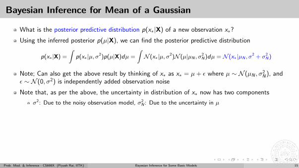
Bayesian Inference for Mean of a Gaussian
What is the posterior predictive distribution p(x∗|X) of a new observation x∗?
Using the inferred posterior p(µ|X), we can find the posterior predictive distribution
p(x∗|X) =
∫p(x∗|µ, σ2)p(µ|X)dµ =
∫N (x∗|µ, σ2)N (µ|µN , σ
2N)dµ = N (x∗|µN , σ
2 + σ2N)
Note; Can also get the above result by thinking of x∗ as x∗ = µ+ ε where µ ∼ N (µN , σ2N), and
ε ∼ N (0, σ2) is independently added observation noise
Note that, as per the above, the uncertainty in distribution of x∗ now has two components
σ2: Due to the noisy observation model, σ2N : Due to the uncertainty in µ
In contrast, the plug-in predictive posterior, given a point estimate µ̂ (e.g., MLE/MAP) would be
p(x∗|X) =
∫p(x∗|µ, σ2)p(µ|X)dµ ≈ p(x∗|µ̂, σ2) = N (x∗|µ̂, σ2)
.. which doesn’t incorporate the uncertainty in our estimate of µ (since we used a point estimate)
Note that as N →∞, both approaches would give the same p(x∗|X) since σ2N → 0
Prob. Mod. & Inference - CS698X (Piyush Rai, IITK) Bayesian Inference for Some Basic Models 15
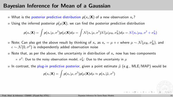
Bayesian Inference for Mean of a Gaussian
What is the posterior predictive distribution p(x∗|X) of a new observation x∗?
Using the inferred posterior p(µ|X), we can find the posterior predictive distribution
p(x∗|X) =
∫p(x∗|µ, σ2)p(µ|X)dµ =
∫N (x∗|µ, σ2)N (µ|µN , σ
2N)dµ = N (x∗|µN , σ
2 + σ2N)
Note; Can also get the above result by thinking of x∗ as x∗ = µ+ ε where µ ∼ N (µN , σ2N), and
ε ∼ N (0, σ2) is independently added observation noise
Note that, as per the above, the uncertainty in distribution of x∗ now has two components
σ2: Due to the noisy observation model, σ2N : Due to the uncertainty in µ
In contrast, the plug-in predictive posterior, given a point estimate µ̂ (e.g., MLE/MAP) would be
p(x∗|X) =
∫p(x∗|µ, σ2)p(µ|X)dµ ≈ p(x∗|µ̂, σ2)
= N (x∗|µ̂, σ2)
.. which doesn’t incorporate the uncertainty in our estimate of µ (since we used a point estimate)
Note that as N →∞, both approaches would give the same p(x∗|X) since σ2N → 0
Prob. Mod. & Inference - CS698X (Piyush Rai, IITK) Bayesian Inference for Some Basic Models 15
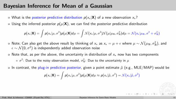
Bayesian Inference for Mean of a Gaussian
What is the posterior predictive distribution p(x∗|X) of a new observation x∗?
Using the inferred posterior p(µ|X), we can find the posterior predictive distribution
p(x∗|X) =
∫p(x∗|µ, σ2)p(µ|X)dµ =
∫N (x∗|µ, σ2)N (µ|µN , σ
2N)dµ = N (x∗|µN , σ
2 + σ2N)
Note; Can also get the above result by thinking of x∗ as x∗ = µ+ ε where µ ∼ N (µN , σ2N), and
ε ∼ N (0, σ2) is independently added observation noise
Note that, as per the above, the uncertainty in distribution of x∗ now has two components
σ2: Due to the noisy observation model, σ2N : Due to the uncertainty in µ
In contrast, the plug-in predictive posterior, given a point estimate µ̂ (e.g., MLE/MAP) would be
p(x∗|X) =
∫p(x∗|µ, σ2)p(µ|X)dµ ≈ p(x∗|µ̂, σ2) = N (x∗|µ̂, σ2)
.. which doesn’t incorporate the uncertainty in our estimate of µ (since we used a point estimate)
Note that as N →∞, both approaches would give the same p(x∗|X) since σ2N → 0
Prob. Mod. & Inference - CS698X (Piyush Rai, IITK) Bayesian Inference for Some Basic Models 15
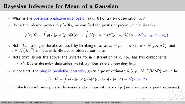
Bayesian Inference for Mean of a Gaussian
What is the posterior predictive distribution p(x∗|X) of a new observation x∗?
Using the inferred posterior p(µ|X), we can find the posterior predictive distribution
p(x∗|X) =
∫p(x∗|µ, σ2)p(µ|X)dµ =
∫N (x∗|µ, σ2)N (µ|µN , σ
2N)dµ = N (x∗|µN , σ
2 + σ2N)
Note; Can also get the above result by thinking of x∗ as x∗ = µ+ ε where µ ∼ N (µN , σ2N), and
ε ∼ N (0, σ2) is independently added observation noise
Note that, as per the above, the uncertainty in distribution of x∗ now has two components
σ2: Due to the noisy observation model, σ2N : Due to the uncertainty in µ
In contrast, the plug-in predictive posterior, given a point estimate µ̂ (e.g., MLE/MAP) would be
p(x∗|X) =
∫p(x∗|µ, σ2)p(µ|X)dµ ≈ p(x∗|µ̂, σ2) = N (x∗|µ̂, σ2)
.. which doesn’t incorporate the uncertainty in our estimate of µ (since we used a point estimate)
Note that as N →∞, both approaches would give the same p(x∗|X) since σ2N → 0
Prob. Mod. & Inference - CS698X (Piyush Rai, IITK) Bayesian Inference for Some Basic Models 15
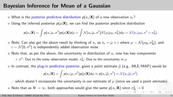
Bayesian Inference for Mean of a Gaussian
What is the posterior predictive distribution p(x∗|X) of a new observation x∗?
Using the inferred posterior p(µ|X), we can find the posterior predictive distribution
p(x∗|X) =
∫p(x∗|µ, σ2)p(µ|X)dµ =
∫N (x∗|µ, σ2)N (µ|µN , σ
2N)dµ = N (x∗|µN , σ
2 + σ2N)
Note; Can also get the above result by thinking of x∗ as x∗ = µ+ ε where µ ∼ N (µN , σ2N), and
ε ∼ N (0, σ2) is independently added observation noise
Note that, as per the above, the uncertainty in distribution of x∗ now has two components
σ2: Due to the noisy observation model, σ2N : Due to the uncertainty in µ
In contrast, the plug-in predictive posterior, given a point estimate µ̂ (e.g., MLE/MAP) would be
p(x∗|X) =
∫p(x∗|µ, σ2)p(µ|X)dµ ≈ p(x∗|µ̂, σ2) = N (x∗|µ̂, σ2)
.. which doesn’t incorporate the uncertainty in our estimate of µ (since we used a point estimate)
Note that as N →∞, both approaches would give the same p(x∗|X) since σ2N → 0
Prob. Mod. & Inference - CS698X (Piyush Rai, IITK) Bayesian Inference for Some Basic Models 15
Bayesian Inference for Variance of a Gaussian
Again consider N i.i.d. observations X = {x1, . . . , xN} drawn from a one-dim Gaussian N (x |µ, σ2)
p(xn|µ, σ2) = N (x |µ, σ2) and p(X|µ, σ2) =N∏
n=1
p(xn|µ, σ2)
Assume the variance σ2 ∈ R+ of the Gaussian is unknown and assume mean µ to be known/fixed
Let’s estimate σ2 given the data X using fully Bayesian inference (not MLE/MAP)
We first need a prior distribution for σ2. What prior p(σ2) to choose in this case?
If we want a conjugate prior, it should have the same form as the likelihood
p(xn|µ, σ2) ∝ (σ2)−1/2 exp
[− (xn − µ)2
2σ2
]An inverse-gamma prior IG (α, β) has this form (α, β are shape and scale hyperparams, resp)
p(σ2) ∝ (σ2)−(α+1) exp
[− β
σ2
](note: mean of IG(α, β) =
β
α− 1)
(Verify) The posterior p(σ2|X) = IG (α + N2 , β +
∑Nn=1(xn−µ)2
2 ). Again IG due to conjugacy.
Prob. Mod. & Inference - CS698X (Piyush Rai, IITK) Bayesian Inference for Some Basic Models 16
Bayesian Inference for Variance of a Gaussian
Again consider N i.i.d. observations X = {x1, . . . , xN} drawn from a one-dim Gaussian N (x |µ, σ2)
p(xn|µ, σ2) = N (x |µ, σ2) and p(X|µ, σ2) =N∏
n=1
p(xn|µ, σ2)
Assume the variance σ2 ∈ R+ of the Gaussian is unknown and assume mean µ to be known/fixed
Let’s estimate σ2 given the data X using fully Bayesian inference (not MLE/MAP)
We first need a prior distribution for σ2. What prior p(σ2) to choose in this case?
If we want a conjugate prior, it should have the same form as the likelihood
p(xn|µ, σ2) ∝ (σ2)−1/2 exp
[− (xn − µ)2
2σ2
]
An inverse-gamma prior IG (α, β) has this form (α, β are shape and scale hyperparams, resp)
p(σ2) ∝ (σ2)−(α+1) exp
[− β
σ2
](note: mean of IG(α, β) =
β
α− 1)
(Verify) The posterior p(σ2|X) = IG (α + N2 , β +
∑Nn=1(xn−µ)2
2 ). Again IG due to conjugacy.
Prob. Mod. & Inference - CS698X (Piyush Rai, IITK) Bayesian Inference for Some Basic Models 16
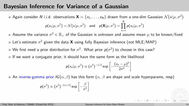
Bayesian Inference for Variance of a Gaussian
Again consider N i.i.d. observations X = {x1, . . . , xN} drawn from a one-dim Gaussian N (x |µ, σ2)
p(xn|µ, σ2) = N (x |µ, σ2) and p(X|µ, σ2) =N∏
n=1
p(xn|µ, σ2)
Assume the variance σ2 ∈ R+ of the Gaussian is unknown and assume mean µ to be known/fixed
Let’s estimate σ2 given the data X using fully Bayesian inference (not MLE/MAP)
We first need a prior distribution for σ2. What prior p(σ2) to choose in this case?
If we want a conjugate prior, it should have the same form as the likelihood
p(xn|µ, σ2) ∝ (σ2)−1/2 exp
[− (xn − µ)2
2σ2
]An inverse-gamma prior IG (α, β) has this form (α, β are shape and scale hyperparams, resp)
p(σ2) ∝ (σ2)−(α+1) exp
[− β
σ2
]
(note: mean of IG(α, β) =β
α− 1)
(Verify) The posterior p(σ2|X) = IG (α + N2 , β +
∑Nn=1(xn−µ)2
2 ). Again IG due to conjugacy.
Prob. Mod. & Inference - CS698X (Piyush Rai, IITK) Bayesian Inference for Some Basic Models 16
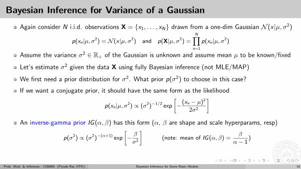
Bayesian Inference for Variance of a Gaussian
Again consider N i.i.d. observations X = {x1, . . . , xN} drawn from a one-dim Gaussian N (x |µ, σ2)
p(xn|µ, σ2) = N (x |µ, σ2) and p(X|µ, σ2) =N∏
n=1
p(xn|µ, σ2)
Assume the variance σ2 ∈ R+ of the Gaussian is unknown and assume mean µ to be known/fixed
Let’s estimate σ2 given the data X using fully Bayesian inference (not MLE/MAP)
We first need a prior distribution for σ2. What prior p(σ2) to choose in this case?
If we want a conjugate prior, it should have the same form as the likelihood
p(xn|µ, σ2) ∝ (σ2)−1/2 exp
[− (xn − µ)2
2σ2
]An inverse-gamma prior IG (α, β) has this form (α, β are shape and scale hyperparams, resp)
p(σ2) ∝ (σ2)−(α+1) exp
[− β
σ2
](note: mean of IG(α, β) =
β
α− 1)
(Verify) The posterior p(σ2|X) = IG (α + N2 , β +
∑Nn=1(xn−µ)2
2 ). Again IG due to conjugacy.
Prob. Mod. & Inference - CS698X (Piyush Rai, IITK) Bayesian Inference for Some Basic Models 16
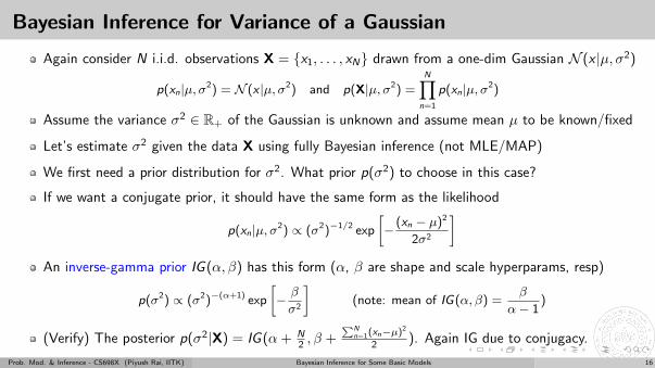
Bayesian Inference for Variance of a Gaussian
Again consider N i.i.d. observations X = {x1, . . . , xN} drawn from a one-dim Gaussian N (x |µ, σ2)
p(xn|µ, σ2) = N (x |µ, σ2) and p(X|µ, σ2) =N∏
n=1
p(xn|µ, σ2)
Assume the variance σ2 ∈ R+ of the Gaussian is unknown and assume mean µ to be known/fixed
Let’s estimate σ2 given the data X using fully Bayesian inference (not MLE/MAP)
We first need a prior distribution for σ2. What prior p(σ2) to choose in this case?
If we want a conjugate prior, it should have the same form as the likelihood
p(xn|µ, σ2) ∝ (σ2)−1/2 exp
[− (xn − µ)2
2σ2
]An inverse-gamma prior IG (α, β) has this form (α, β are shape and scale hyperparams, resp)
p(σ2) ∝ (σ2)−(α+1) exp
[− β
σ2
](note: mean of IG(α, β) =
β
α− 1)
(Verify) The posterior p(σ2|X) = IG (α + N2 , β +
∑Nn=1(xn−µ)2
2 ). Again IG due to conjugacy.
Prob. Mod. & Inference - CS698X (Piyush Rai, IITK) Bayesian Inference for Some Basic Models 16
Working with Gaussians: Variance vs Precision
Often, it is easier to work with the precision (=1/variance) rather than variance
p(xn|µ, τ) = N (x |µ, τ) =
√τ
2πexp
[−τ
2(xn − µ)2
]
If mean is known, for precision Gamma(α, β) is a conjugate prior to Gaussian likelihood
p(τ) ∝ (τ)(α−1) exp [−βτ ] (note: mean of Gamma(α, β) =α
β)
.. where α and β are the shape and rate hyperparamers, respectively, for the Gamma
(Verify) The posterior p(τ |X) will also be Gamma(α + N2 , β +
∑Nn=1(xn−µ)2
2 )
Note: Gamma distribution can be defined in terms of shape and scale or shape and rateparametrization (scale = 1/rate). Likewise, inverse Gamma can also be defined both shape andscale (which we saw) as well as shape and rate parametrizations.
Prob. Mod. & Inference - CS698X (Piyush Rai, IITK) Bayesian Inference for Some Basic Models 17
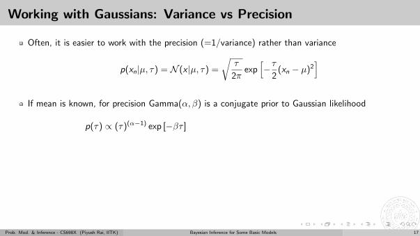
Working with Gaussians: Variance vs Precision
Often, it is easier to work with the precision (=1/variance) rather than variance
p(xn|µ, τ) = N (x |µ, τ) =
√τ
2πexp
[−τ
2(xn − µ)2
]
If mean is known, for precision Gamma(α, β) is a conjugate prior to Gaussian likelihood
p(τ) ∝ (τ)(α−1) exp [−βτ ]
(note: mean of Gamma(α, β) =α
β)
.. where α and β are the shape and rate hyperparamers, respectively, for the Gamma
(Verify) The posterior p(τ |X) will also be Gamma(α + N2 , β +
∑Nn=1(xn−µ)2
2 )
Note: Gamma distribution can be defined in terms of shape and scale or shape and rateparametrization (scale = 1/rate). Likewise, inverse Gamma can also be defined both shape andscale (which we saw) as well as shape and rate parametrizations.
Prob. Mod. & Inference - CS698X (Piyush Rai, IITK) Bayesian Inference for Some Basic Models 17
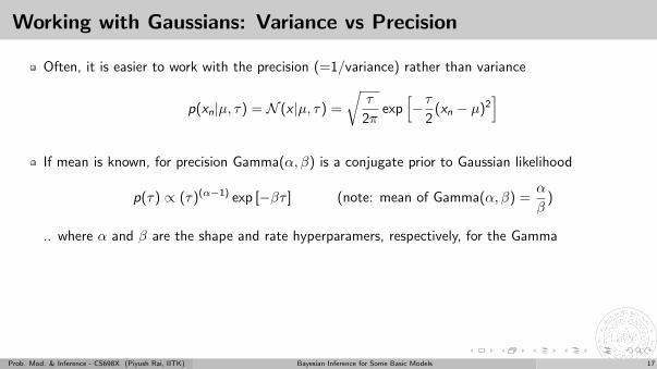
Working with Gaussians: Variance vs Precision
Often, it is easier to work with the precision (=1/variance) rather than variance
p(xn|µ, τ) = N (x |µ, τ) =
√τ
2πexp
[−τ
2(xn − µ)2
]
If mean is known, for precision Gamma(α, β) is a conjugate prior to Gaussian likelihood
p(τ) ∝ (τ)(α−1) exp [−βτ ] (note: mean of Gamma(α, β) =α
β)
.. where α and β are the shape and rate hyperparamers, respectively, for the Gamma
(Verify) The posterior p(τ |X) will also be Gamma(α + N2 , β +
∑Nn=1(xn−µ)2
2 )
Note: Gamma distribution can be defined in terms of shape and scale or shape and rateparametrization (scale = 1/rate). Likewise, inverse Gamma can also be defined both shape andscale (which we saw) as well as shape and rate parametrizations.
Prob. Mod. & Inference - CS698X (Piyush Rai, IITK) Bayesian Inference for Some Basic Models 17
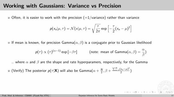
Working with Gaussians: Variance vs Precision
Often, it is easier to work with the precision (=1/variance) rather than variance
p(xn|µ, τ) = N (x |µ, τ) =
√τ
2πexp
[−τ
2(xn − µ)2
]
If mean is known, for precision Gamma(α, β) is a conjugate prior to Gaussian likelihood
p(τ) ∝ (τ)(α−1) exp [−βτ ] (note: mean of Gamma(α, β) =α
β)
.. where α and β are the shape and rate hyperparamers, respectively, for the Gamma
(Verify) The posterior p(τ |X) will also be Gamma(α + N2 , β +
∑Nn=1(xn−µ)2
2 )
Note: Gamma distribution can be defined in terms of shape and scale or shape and rateparametrization (scale = 1/rate). Likewise, inverse Gamma can also be defined both shape andscale (which we saw) as well as shape and rate parametrizations.
Prob. Mod. & Inference - CS698X (Piyush Rai, IITK) Bayesian Inference for Some Basic Models 17
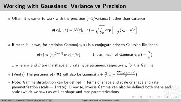
Working with Gaussians: Variance vs Precision
Often, it is easier to work with the precision (=1/variance) rather than variance
p(xn|µ, τ) = N (x |µ, τ) =
√τ
2πexp
[−τ
2(xn − µ)2
]
If mean is known, for precision Gamma(α, β) is a conjugate prior to Gaussian likelihood
p(τ) ∝ (τ)(α−1) exp [−βτ ] (note: mean of Gamma(α, β) =α
β)
.. where α and β are the shape and rate hyperparamers, respectively, for the Gamma
(Verify) The posterior p(τ |X) will also be Gamma(α + N2 , β +
∑Nn=1(xn−µ)2
2 )
Note: Gamma distribution can be defined in terms of shape and scale or shape and rateparametrization (scale = 1/rate). Likewise, inverse Gamma can also be defined both shape andscale (which we saw) as well as shape and rate parametrizations.
Prob. Mod. & Inference - CS698X (Piyush Rai, IITK) Bayesian Inference for Some Basic Models 17
Bayesian Inference for Both Parameters of a Gaussian!
Gaussian with unknown scalar mean and unknown scalar precision (two parameters)
Consider N i.i.d. observations X = {x1, . . . , xN} drawn from a one-dim Gaussian N (x |µ, λ−1)
Assume both mean µ and precision λ to be unknown. The likelihood will be
p(X|µ, λ) =N∏
n=1
√λ
2πexp
[−λ
2(xn − µ)2
]
∝[λ1/2 exp
(−λµ
2
2
)]Nexp
[λµ
N∑n=1
xn −λ
2
N∑n=1
x2n
]If we want a conjugate joint prior p(µ, λ), it must have the same form as likelihood. Suppose
p(µ, λ) ∝[λ1/2 exp
(−λµ
2
2
)]κ0
exp [λµc − λd ]
What’s this prior? A normal-gamma (Gaussian-gamma) distribution! (will see its form shortly)
Can be used when we wish to estimate the unknown mean and unknown precision of a Gaussian
Note: Its multivariate version is the Normal-Wishart (for multivariate mean and precision matrix)
Prob. Mod. & Inference - CS698X (Piyush Rai, IITK) Bayesian Inference for Some Basic Models 18
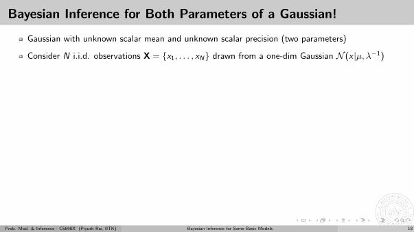
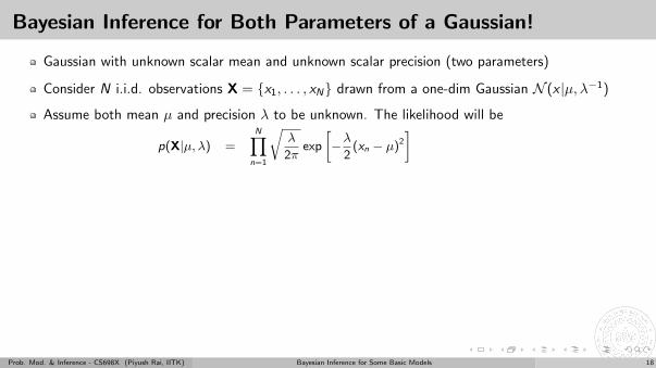
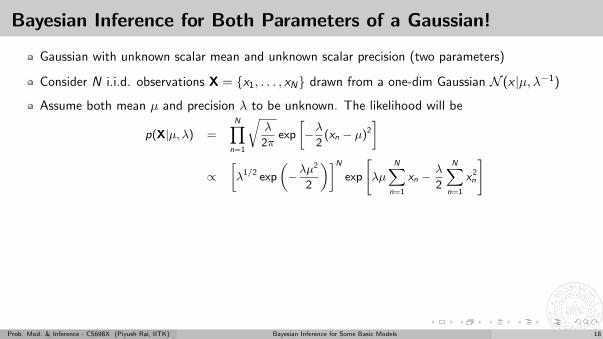
Bayesian Inference for Both Parameters of a Gaussian!
Gaussian with unknown scalar mean and unknown scalar precision (two parameters)
Consider N i.i.d. observations X = {x1, . . . , xN} drawn from a one-dim Gaussian N (x |µ, λ−1)
Assume both mean µ and precision λ to be unknown. The likelihood will be
p(X|µ, λ) =N∏
n=1
√λ
2πexp
[−λ
2(xn − µ)2
]
∝[λ1/2 exp
(−λµ
2
2
)]Nexp
[λµ
N∑n=1
xn −λ
2
N∑n=1
x2n
]
If we want a conjugate joint prior p(µ, λ), it must have the same form as likelihood. Suppose
p(µ, λ) ∝[λ1/2 exp
(−λµ
2
2
)]κ0
exp [λµc − λd ]
What’s this prior? A normal-gamma (Gaussian-gamma) distribution! (will see its form shortly)
Can be used when we wish to estimate the unknown mean and unknown precision of a Gaussian
Note: Its multivariate version is the Normal-Wishart (for multivariate mean and precision matrix)
Prob. Mod. & Inference - CS698X (Piyush Rai, IITK) Bayesian Inference for Some Basic Models 18
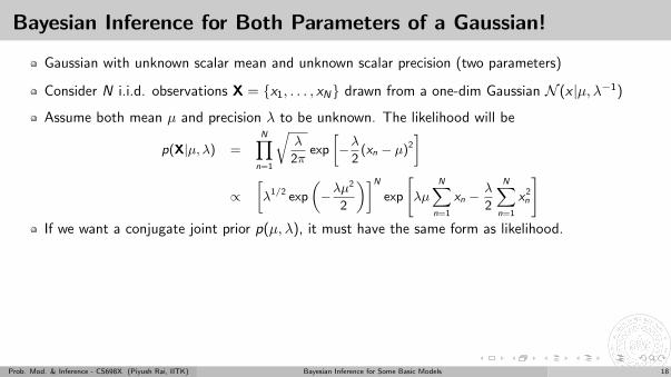
Bayesian Inference for Both Parameters of a Gaussian!
Gaussian with unknown scalar mean and unknown scalar precision (two parameters)
Consider N i.i.d. observations X = {x1, . . . , xN} drawn from a one-dim Gaussian N (x |µ, λ−1)
Assume both mean µ and precision λ to be unknown. The likelihood will be
p(X|µ, λ) =N∏
n=1
√λ
2πexp
[−λ
2(xn − µ)2
]
∝[λ1/2 exp
(−λµ
2
2
)]Nexp
[λµ
N∑n=1
xn −λ
2
N∑n=1
x2n
]If we want a conjugate joint prior p(µ, λ), it must have the same form as likelihood.
Suppose
p(µ, λ) ∝[λ1/2 exp
(−λµ
2
2
)]κ0
exp [λµc − λd ]
What’s this prior? A normal-gamma (Gaussian-gamma) distribution! (will see its form shortly)
Can be used when we wish to estimate the unknown mean and unknown precision of a Gaussian
Note: Its multivariate version is the Normal-Wishart (for multivariate mean and precision matrix)
Prob. Mod. & Inference - CS698X (Piyush Rai, IITK) Bayesian Inference for Some Basic Models 18
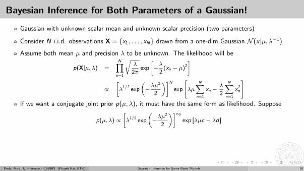
Bayesian Inference for Both Parameters of a Gaussian!
Gaussian with unknown scalar mean and unknown scalar precision (two parameters)
Consider N i.i.d. observations X = {x1, . . . , xN} drawn from a one-dim Gaussian N (x |µ, λ−1)
Assume both mean µ and precision λ to be unknown. The likelihood will be
p(X|µ, λ) =N∏
n=1
√λ
2πexp
[−λ
2(xn − µ)2
]
∝[λ1/2 exp
(−λµ
2
2
)]Nexp
[λµ
N∑n=1
xn −λ
2
N∑n=1
x2n
]If we want a conjugate joint prior p(µ, λ), it must have the same form as likelihood. Suppose
p(µ, λ) ∝[λ1/2 exp
(−λµ
2
2
)]κ0
exp [λµc − λd ]
What’s this prior? A normal-gamma (Gaussian-gamma) distribution! (will see its form shortly)
Can be used when we wish to estimate the unknown mean and unknown precision of a Gaussian
Note: Its multivariate version is the Normal-Wishart (for multivariate mean and precision matrix)
Prob. Mod. & Inference - CS698X (Piyush Rai, IITK) Bayesian Inference for Some Basic Models 18
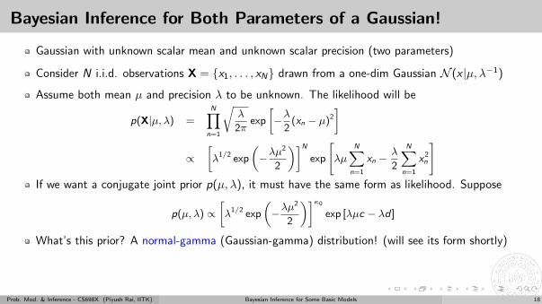
Bayesian Inference for Both Parameters of a Gaussian!
Gaussian with unknown scalar mean and unknown scalar precision (two parameters)
Consider N i.i.d. observations X = {x1, . . . , xN} drawn from a one-dim Gaussian N (x |µ, λ−1)
Assume both mean µ and precision λ to be unknown. The likelihood will be
p(X|µ, λ) =N∏
n=1
√λ
2πexp
[−λ
2(xn − µ)2
]
∝[λ1/2 exp
(−λµ
2
2
)]Nexp
[λµ
N∑n=1
xn −λ
2
N∑n=1
x2n
]If we want a conjugate joint prior p(µ, λ), it must have the same form as likelihood. Suppose
p(µ, λ) ∝[λ1/2 exp
(−λµ
2
2
)]κ0
exp [λµc − λd ]
What’s this prior? A normal-gamma (Gaussian-gamma) distribution! (will see its form shortly)
Can be used when we wish to estimate the unknown mean and unknown precision of a Gaussian
Note: Its multivariate version is the Normal-Wishart (for multivariate mean and precision matrix)
Prob. Mod. & Inference - CS698X (Piyush Rai, IITK) Bayesian Inference for Some Basic Models 18
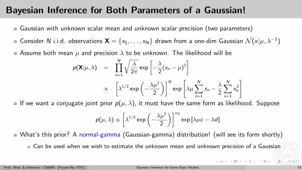
Bayesian Inference for Both Parameters of a Gaussian!
Gaussian with unknown scalar mean and unknown scalar precision (two parameters)
Consider N i.i.d. observations X = {x1, . . . , xN} drawn from a one-dim Gaussian N (x |µ, λ−1)
Assume both mean µ and precision λ to be unknown. The likelihood will be
p(X|µ, λ) =N∏
n=1
√λ
2πexp
[−λ
2(xn − µ)2
]
∝[λ1/2 exp
(−λµ
2
2
)]Nexp
[λµ
N∑n=1
xn −λ
2
N∑n=1
x2n
]If we want a conjugate joint prior p(µ, λ), it must have the same form as likelihood. Suppose
p(µ, λ) ∝[λ1/2 exp
(−λµ
2
2
)]κ0
exp [λµc − λd ]
What’s this prior? A normal-gamma (Gaussian-gamma) distribution! (will see its form shortly)
Can be used when we wish to estimate the unknown mean and unknown precision of a Gaussian
Note: Its multivariate version is the Normal-Wishart (for multivariate mean and precision matrix)
Prob. Mod. & Inference - CS698X (Piyush Rai, IITK) Bayesian Inference for Some Basic Models 18
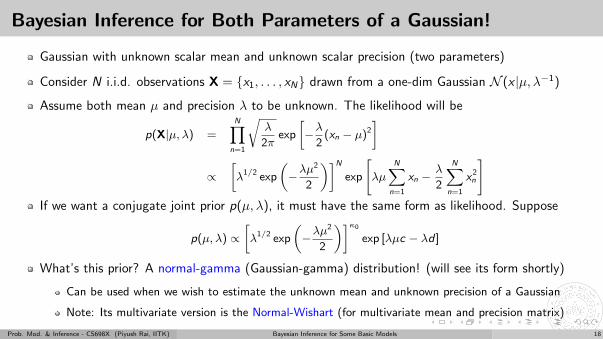
Bayesian Inference for Both Parameters of a Gaussian!
Gaussian with unknown scalar mean and unknown scalar precision (two parameters)
Consider N i.i.d. observations X = {x1, . . . , xN} drawn from a one-dim Gaussian N (x |µ, λ−1)
Assume both mean µ and precision λ to be unknown. The likelihood will be
p(X|µ, λ) =N∏
n=1
√λ
2πexp
[−λ
2(xn − µ)2
]
∝[λ1/2 exp
(−λµ
2
2
)]Nexp
[λµ
N∑n=1
xn −λ
2
N∑n=1
x2n
]If we want a conjugate joint prior p(µ, λ), it must have the same form as likelihood. Suppose
p(µ, λ) ∝[λ1/2 exp
(−λµ
2
2
)]κ0
exp [λµc − λd ]
What’s this prior? A normal-gamma (Gaussian-gamma) distribution! (will see its form shortly)
Can be used when we wish to estimate the unknown mean and unknown precision of a Gaussian
Note: Its multivariate version is the Normal-Wishart (for multivariate mean and precision matrix)
Prob. Mod. & Inference - CS698X (Piyush Rai, IITK) Bayesian Inference for Some Basic Models 18
Normal-gamma (Gaussian-gamma) Distribution
We saw that the conjugate prior needed to have the form
p(µ, λ) ∝[λ1/2 exp
(−λµ
2
2
)]κ0
exp [λµc − λd ]
= exp
[−κ0λ
2(µ− c/κ0)2
]︸ ︷︷ ︸
prop. to a Gaussian
λκ0/2 exp
[−(d − c2
2κ0
)λ
]︸ ︷︷ ︸
prop. to a gamma
(re-arranging terms)
The above is product of a normal and a gamma distribution1
p(µ, λ) = N (µ|µ0, (κ0λ)−1)Gamma(λ|α0, β0) = NG(µ0, κ0, α0, β0)
where µ0 = c/κ0, α0 = 1 + κ0/2, β0 = d − c2/2κ0 are prior’s hyperparameters
p(µ, λ) = NG(µ0, κ0, α0, β0) is a conjugate for the mean-precision pair (µ, λ)
A useful prior in many problems involving Gaussians with unknown mean and precision
1shape-rate parametrization assumed for the gamma
Prob. Mod. & Inference - CS698X (Piyush Rai, IITK) Bayesian Inference for Some Basic Models 19
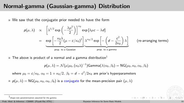
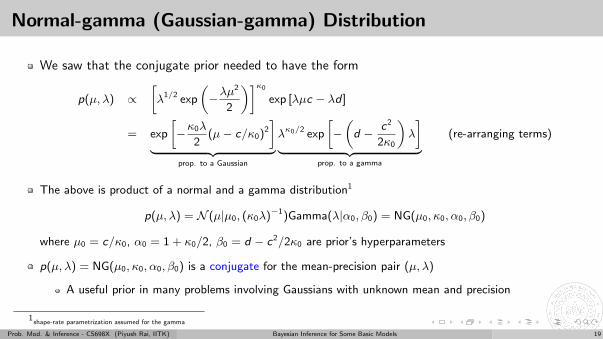
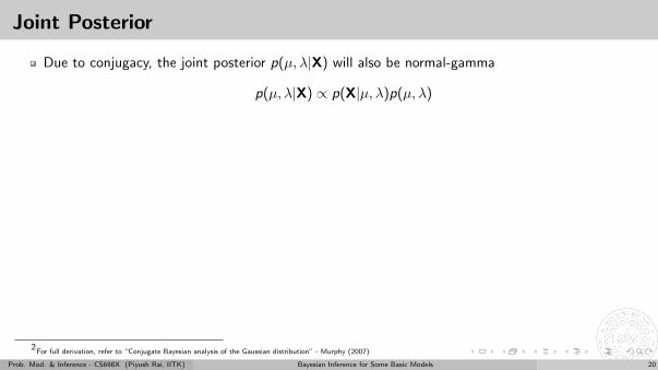
Joint Posterior
Due to conjugacy, the joint posterior p(µ, λ|X) will also be normal-gamma
p(µ, λ|X) ∝ p(X|µ, λ)p(µ, λ)
Plugging in the expressions for p(X|µ, λ) and p(µ, λ), we get
p(µ, λ|X) = NG(µN , κN , αN , βN) = N (µ|µN , (κNλ)−1)Gamma(λ|αN , βN)
where the updated posterior hyperparameters are given by2
µN =κ0µ0 + Nx̄
κ0 + NκN = κ0 + N
αN = α0 + N/2
βN = β0 +1
2
N∑n=1
(xn − x̄)2 +κ0N(x̄ − µ0)2
2(κ0 + N)
2For full derivation, refer to “Conjugate Bayesian analysis of the Gaussian distribution” - Murphy (2007)
Prob. Mod. & Inference - CS698X (Piyush Rai, IITK) Bayesian Inference for Some Basic Models 20
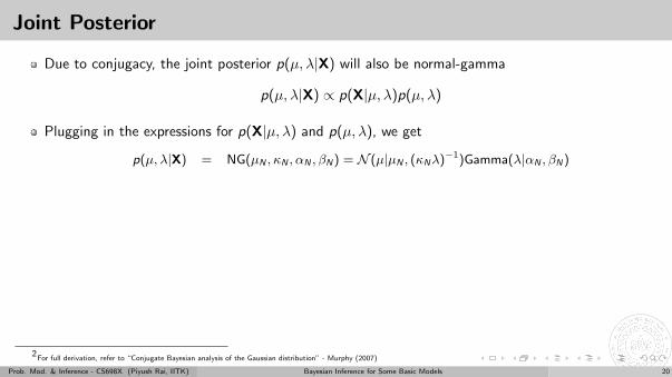
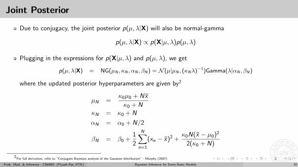
Other Quantities of Interest3
Already saw that joint post. p(µ, λ|X) = NG(µN , κN , αN , βN) = N (µ|µN , (κNλ)−1)Gamma(λ|αN , βN)
Marginal posteriors for µ and λ
p(λ|X) =
∫p(µ, λ|X)dµ = Gamma(λ|αN , βN )
p(µ|X) =
∫p(µ, λ|X)dλ =
∫p(µ|λ,X)p(λ|X)dλ = t2αN
(µ|µN , βN/(αNκN ))︸ ︷︷ ︸t distribution
Exercise: What will be the conditional posteriors p(µ|λ,X) and p(λ|µ,X)?
Marginal likelihood of the model
p(X) =Γ(αN )
Γ(α0)
βα00
βαNN
(κ0
κN
) 12
(2π)−N/2
Posterior predictive distribution of a new observation x∗
p(x∗|X) =
∫p(x∗|µ, λ)︸ ︷︷ ︸
Gaussian
p(µ, λ|X)︸ ︷︷ ︸Normal-Gamma
dµdλ = t2αN
(x∗|µN ,
βN (κN + 1)
αNκN
)
3For full derivations, refer to “Conjugate Bayesian analysis of the Gaussian distribution” - Murphy (2007)
Prob. Mod. & Inference - CS698X (Piyush Rai, IITK) Bayesian Inference for Some Basic Models 21
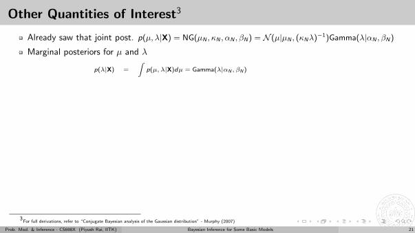
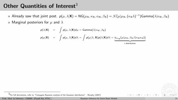
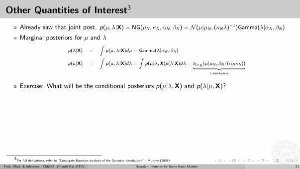
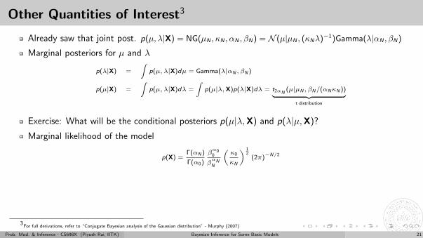
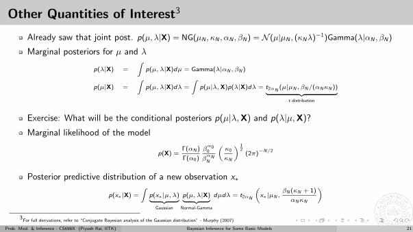
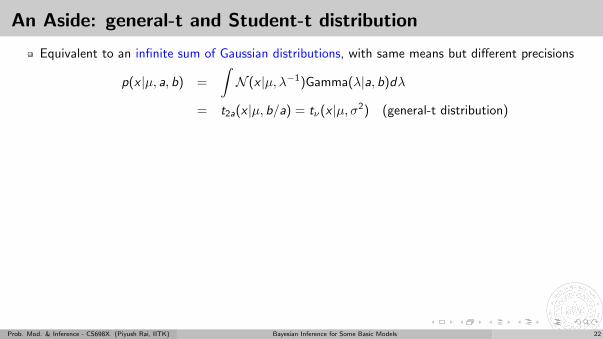
An Aside: general-t and Student-t distribution
Equivalent to an infinite sum of Gaussian distributions, with same means but different precisions
p(x |µ, a, b) =
∫N (x |µ, λ−1)Gamma(λ|a, b)dλ
= t2a(x |µ, b/a) = tν(x |µ, σ2) (general-t distribution)
µ = 0, σ2 = 1 gives the Student-t distribution (tν). Note: If x ∼ tν(µ, σ2) then x−µσ ∼ tν
An illustration of student-t
t distribution has a “fatter” tail than a Gaussian and also sharper around the mean
Also a useful prior for sparse modeling
Prob. Mod. & Inference - CS698X (Piyush Rai, IITK) Bayesian Inference for Some Basic Models 22
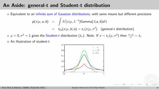
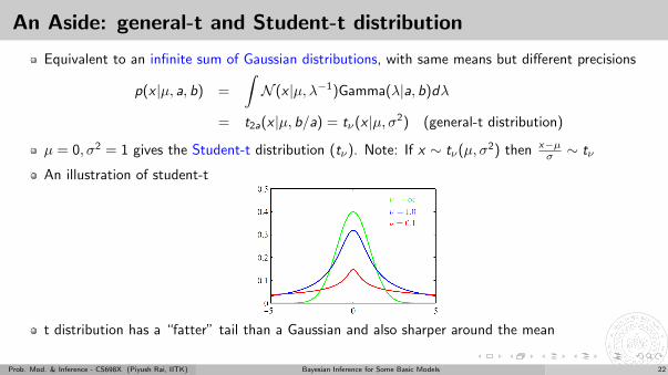
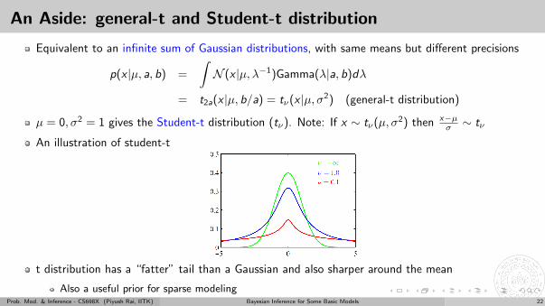
An Aside: general-t and Student-t distribution
Equivalent to an infinite sum of Gaussian distributions, with same means but different precisions
p(x |µ, a, b) =
∫N (x |µ, λ−1)Gamma(λ|a, b)dλ
= t2a(x |µ, b/a) = tν(x |µ, σ2) (general-t distribution)
µ = 0, σ2 = 1 gives the Student-t distribution (tν). Note: If x ∼ tν(µ, σ2) then x−µσ ∼ tν
An illustration of student-t
t distribution has a “fatter” tail than a Gaussian and also sharper around the mean
Also a useful prior for sparse modelingProb. Mod. & Inference - CS698X (Piyush Rai, IITK) Bayesian Inference for Some Basic Models 22
Inferring Parameters of Gaussian: Some Other Cases
We only considered the simple 1-D Gaussian distribution
The approach also extends to inferring parameters of a multivariate Gaussian
For the unknown mean and precision matrix, normal-Wishart distribution can be used as prior
Posterior updates have forms similar to that in the 1-D case
When working with mean-variance, we can use normal-inverse gamma as conjugate prior (ornormal-inverse Wishart when working with mean-covariance matrix in case of multivariate Gaussiandistribution)
Other priors can also be used as well when inferring parameters of Gaussians, e.g.,
normal-Inverse χ2 distribution is commonly used in Statistics community for scalar mean-variance
Uniform priors can also be used
Look at BDA Chapter 3 for such examples
Also refer to “Conjugate Bayesian analysis of the Gaussian distribution” - Murphy (2007) forvarious examples and more detailed derivations
Prob. Mod. & Inference - CS698X (Piyush Rai, IITK) Bayesian Inference for Some Basic Models 23
Inferring Parameters of Gaussian: Some Other Cases
We only considered the simple 1-D Gaussian distribution
The approach also extends to inferring parameters of a multivariate Gaussian
For the unknown mean and precision matrix, normal-Wishart distribution can be used as prior
Posterior updates have forms similar to that in the 1-D case
When working with mean-variance, we can use normal-inverse gamma as conjugate prior (ornormal-inverse Wishart when working with mean-covariance matrix in case of multivariate Gaussiandistribution)
Other priors can also be used as well when inferring parameters of Gaussians
, e.g.,
normal-Inverse χ2 distribution is commonly used in Statistics community for scalar mean-variance
Uniform priors can also be used
Look at BDA Chapter 3 for such examples
Also refer to “Conjugate Bayesian analysis of the Gaussian distribution” - Murphy (2007) forvarious examples and more detailed derivations
Prob. Mod. & Inference - CS698X (Piyush Rai, IITK) Bayesian Inference for Some Basic Models 23
Inferring Parameters of Gaussian: Some Other Cases
We only considered the simple 1-D Gaussian distribution
The approach also extends to inferring parameters of a multivariate Gaussian
For the unknown mean and precision matrix, normal-Wishart distribution can be used as prior
Posterior updates have forms similar to that in the 1-D case
When working with mean-variance, we can use normal-inverse gamma as conjugate prior (ornormal-inverse Wishart when working with mean-covariance matrix in case of multivariate Gaussiandistribution)
Other priors can also be used as well when inferring parameters of Gaussians, e.g.,
normal-Inverse χ2 distribution is commonly used in Statistics community for scalar mean-variance
Uniform priors can also be used
Look at BDA Chapter 3 for such examples
Also refer to “Conjugate Bayesian analysis of the Gaussian distribution” - Murphy (2007) forvarious examples and more detailed derivations
Prob. Mod. & Inference - CS698X (Piyush Rai, IITK) Bayesian Inference for Some Basic Models 23
Inferring Parameters of Gaussian: Some Other Cases
We only considered the simple 1-D Gaussian distribution
The approach also extends to inferring parameters of a multivariate Gaussian
For the unknown mean and precision matrix, normal-Wishart distribution can be used as prior
Posterior updates have forms similar to that in the 1-D case
When working with mean-variance, we can use normal-inverse gamma as conjugate prior (ornormal-inverse Wishart when working with mean-covariance matrix in case of multivariate Gaussiandistribution)
Other priors can also be used as well when inferring parameters of Gaussians, e.g.,
normal-Inverse χ2 distribution is commonly used in Statistics community for scalar mean-variance
Uniform priors can also be used
Look at BDA Chapter 3 for such examples
Also refer to “Conjugate Bayesian analysis of the Gaussian distribution” - Murphy (2007) forvarious examples and more detailed derivations
Prob. Mod. & Inference - CS698X (Piyush Rai, IITK) Bayesian Inference for Some Basic Models 23
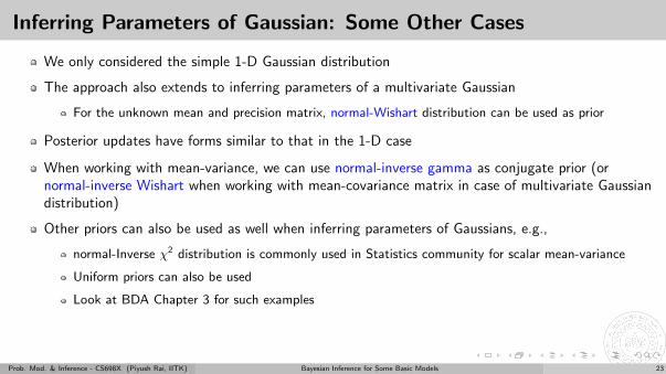
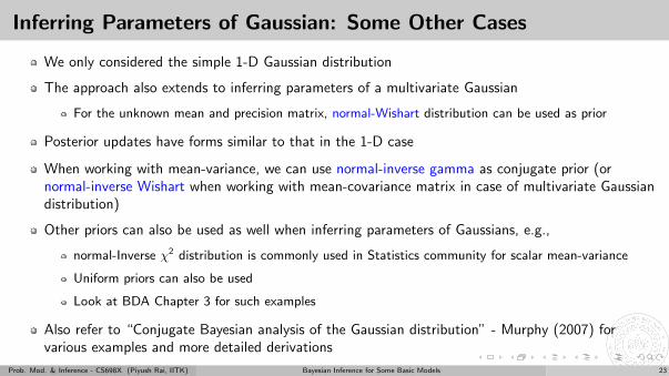
Next Class: More examples of Bayesian inferencewith Gaussians
Prob. Mod. & Inference - CS698X (Piyush Rai, IITK) Bayesian Inference for Some Basic Models 24
Top Related