Approximation Bounds for

Sparse Principal Component Analysis

Alexandre d’Aspremont, CNRS & Ecole Polytechnique.

With Francis Bach, INRIA-ENS and Laurent El Ghaoui, U.C. Berkeley.

Support from NSF, ERC and Google.

A. d’Aspremont IHP, May 2013. 1/31

Introduction

High dimensional data sets. n sample points in dimension p, with

p = γn, p→∞.

for some fixed γ > 0.

� Common in e.g. biology (many genes, few samples), or finance (data notstationary, many assets).

� Many recent results on PCA in this setting. Very precise knowledge ofasymptotic distributions of extremal eigenvalues.

� Test the significance of principal eigenvalues.

A. d’Aspremont IHP, May 2013. 2/31

Introduction

Sample covariance matrix in a high dimensional setting.

� If the entries of X ∈ Rn×p are standard i.i.d. and have a fourth moment, then

λmax

(XTX

n− 1

)→ (1 +

√γ)2 a.s.

if p = γn, p→∞. [Geman, 1980, Yin et al., 1988]

� When γ ∈ (0, 1], the spectral measure converges to the following density

fγ =

√(x− a)(b− x)

2πγx

where a = (1−√γ)2 and b = (1 +√γ)2. [Marcenko and Pastur, 1967]

� The distribution of λmax

(XTXn−1

), properly normalized, converges to the

Tracy-Widom distribution [Johnstone, 2001, Karoui, 2003]. This works welleven for small values of n, p.

A. d’Aspremont IHP, May 2013. 3/31

Introduction

0 100 200 300 400 500

0.5

1

1.5

2

i

λi

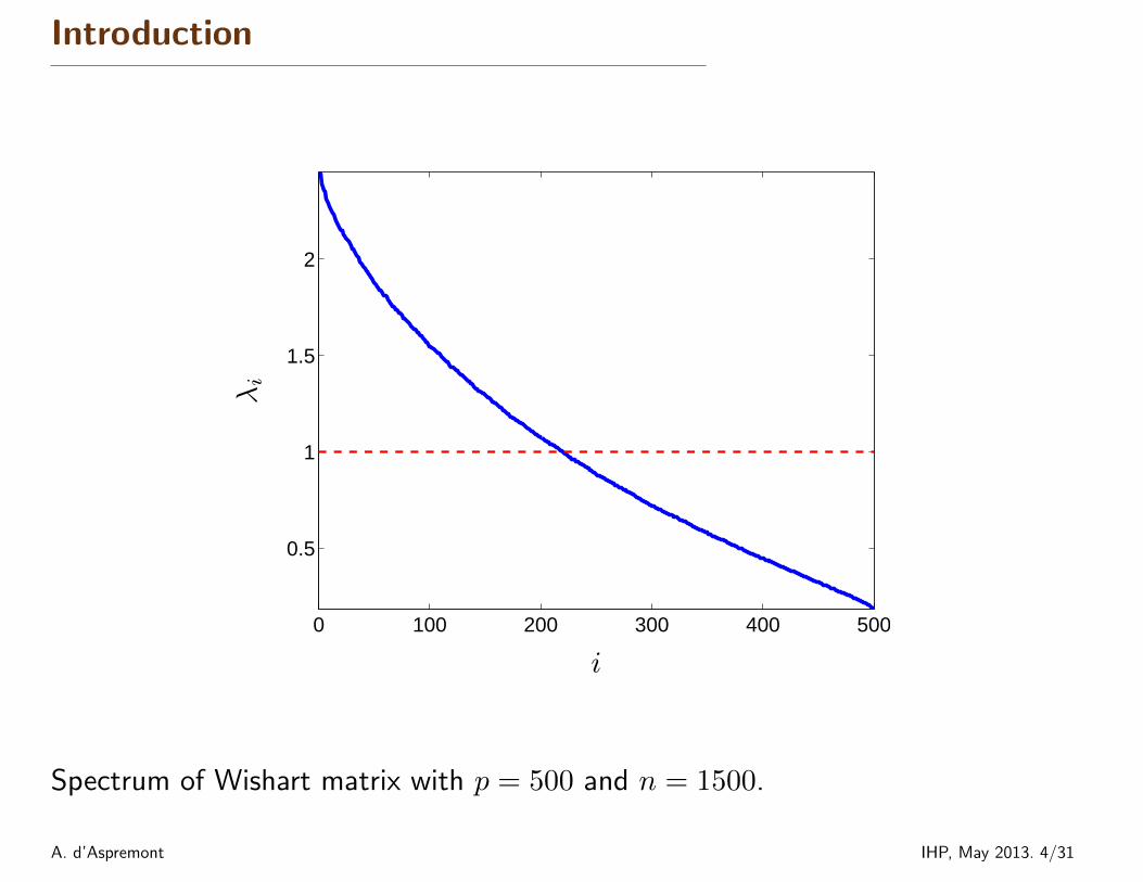
Spectrum of Wishart matrix with p = 500 and n = 1500.

A. d’Aspremont IHP, May 2013. 4/31

Introduction

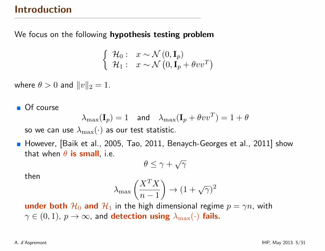
We focus on the following hypothesis testing problem{H0 : x ∼ N (0, Ip)H1 : x ∼ N

(0, Ip + θvvT

)where θ > 0 and ‖v‖2 = 1.

� Of courseλmax(Ip) = 1 and λmax(Ip + θvvT ) = 1 + θ

so we can use λmax(·) as our test statistic.

� However, [Baik et al., 2005, Tao, 2011, Benaych-Georges et al., 2011] showthat when θ is small, i.e.

θ ≤ γ +√γ

then

λmax

(XTX

n− 1

)→ (1 +

√γ)2

under both H0 and H1 in the high dimensional regime p = γn, withγ ∈ (0, 1), p→∞, and detection using λmax(·) fails.

A. d’Aspremont IHP, May 2013. 5/31

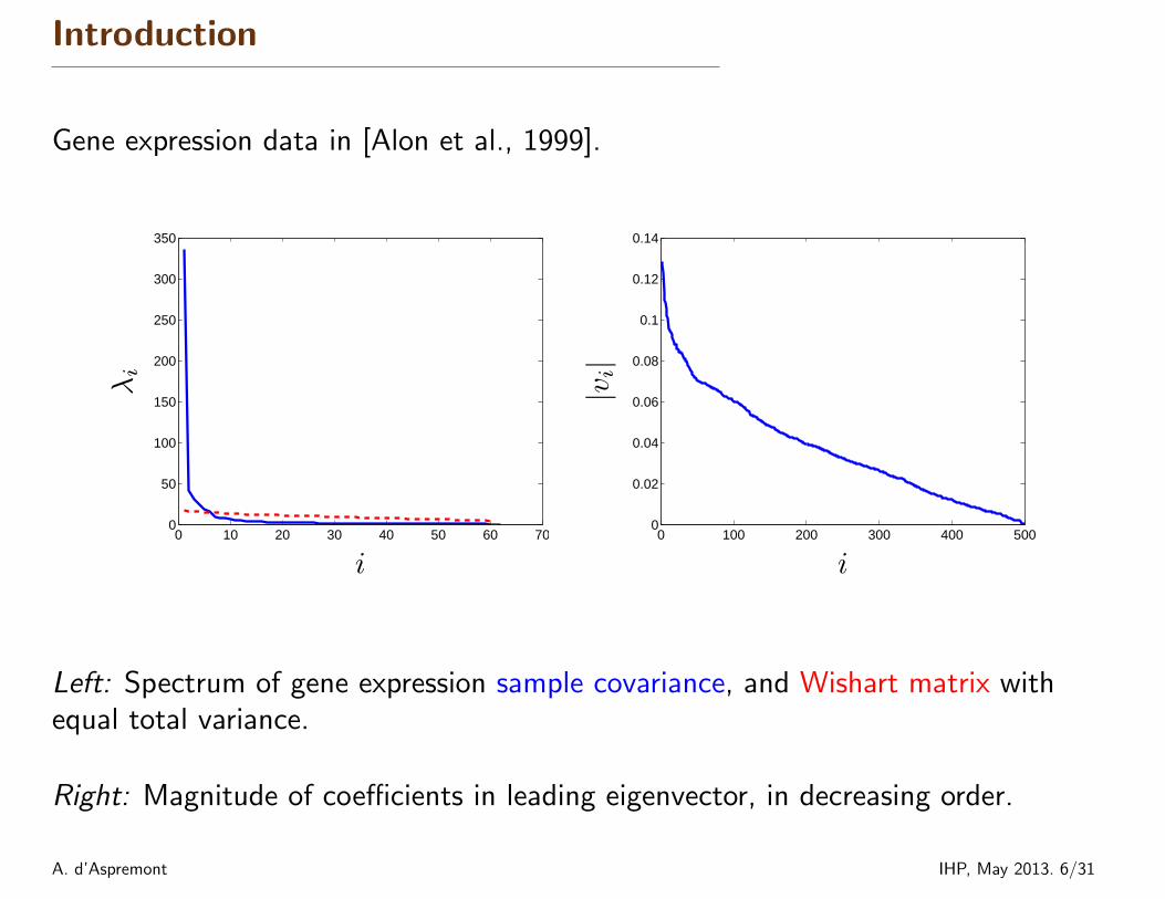
Introduction

Gene expression data in [Alon et al., 1999].

0 10 20 30 40 50 60 700

50

100

150

200

250

300

350

i

λi

0 100 200 300 400 5000

0.02

0.04

0.06

0.08

0.1

0.12

0.14

i|v

i|

Left: Spectrum of gene expression sample covariance, and Wishart matrix withequal total variance.

Right: Magnitude of coefficients in leading eigenvector, in decreasing order.

A. d’Aspremont IHP, May 2013. 6/31

Introduction

Here, we assume the leading principal component is sparse. We will use sparseeigenvalues as a test statistic

λkmax(Σ) , max. xTΣxs.t. Card(x) ≤ k

‖x‖2 = 1,

� We focus on the sparse eigenvector detection problem{H0 : x ∼ N (0, Ip)H1 : x ∼ N

(0, Ip + θvvT

)where θ > 0 and ‖v‖2 = 1 with Card(v) = k.

� We naturally have

λkmax(Ip) = 1 and λkmax(Ip + θvvT ) = 1 + θ

A. d’Aspremont IHP, May 2013. 7/31

Introduction

Berthet and Rigollet [2012] show the following results on the detection threshold

� Under H1:

λkmax(Σ) ≥ 1 + θ − 2(1 + θ)

√log(1/δ)

nwith probability 1− δ.

� Under H0:

λkmax(Σ) ≤ 1 + 4

√k log(9ep/k) + log(1/δ)

n+ 4

k log(9ep/k) + log(1/δ)

n

with probability 1− δ.

This means that the detection threshold is

θ = 4

√k log(9ep/k) + log(1/δ)

n+ 4

k log(9ep/k) + log(1/δ)

n+ 4

√log(1/δ)

n

which is minimax optimal [Berthet and Rigollet, 2012, Th. 5.1].

A. d’Aspremont IHP, May 2013. 8/31

Sparse PCA

Optimal detection threshold using λkmax(·) is

θ = 4

√k log(9ep/k)

n+ . . .

� Good news: λkmax(·) is a minimax optimal statistic for detecting sparseprincipal components. The dimension p only appears as a log term and thisthreshold is much better than θ =

√p/n in the dense PCA case.

� Bad news: Computing the statistic λkmax(Σ) is NP-Hard.

[Berthet and Rigollet, 2012] produce tractable statistics achieving the threshold

θ = 2√k

√k log(4p2/δ)

n+ . . .

which means θ →∞ when k, n, p→∞ proportionally. However p large, k fixed isOK, empirical performance much better than this bound would predict.

A. d’Aspremont IHP, May 2013. 9/31

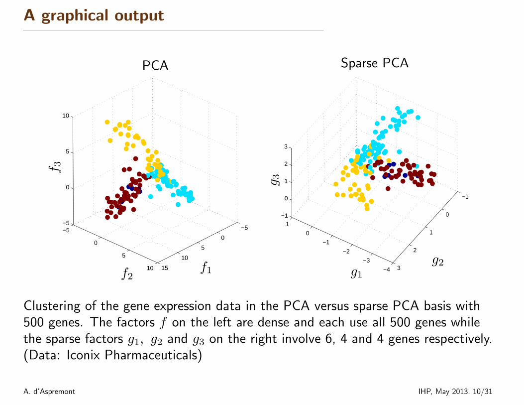
A graphical output

−5

0

5

10

15

−5

0

5

10

−5

0

5

10

−4

−3

−2

−1

0

1

−1

0

1

2

3

−1

0

1

2

3

f1f2

f 3

g1g2

g 3

PCA Sparse PCA

Clustering of the gene expression data in the PCA versus sparse PCA basis with500 genes. The factors f on the left are dense and each use all 500 genes whilethe sparse factors g1, g2 and g3 on the right involve 6, 4 and 4 genes respectively.(Data: Iconix Pharmaceuticals)

A. d’Aspremont IHP, May 2013. 10/31

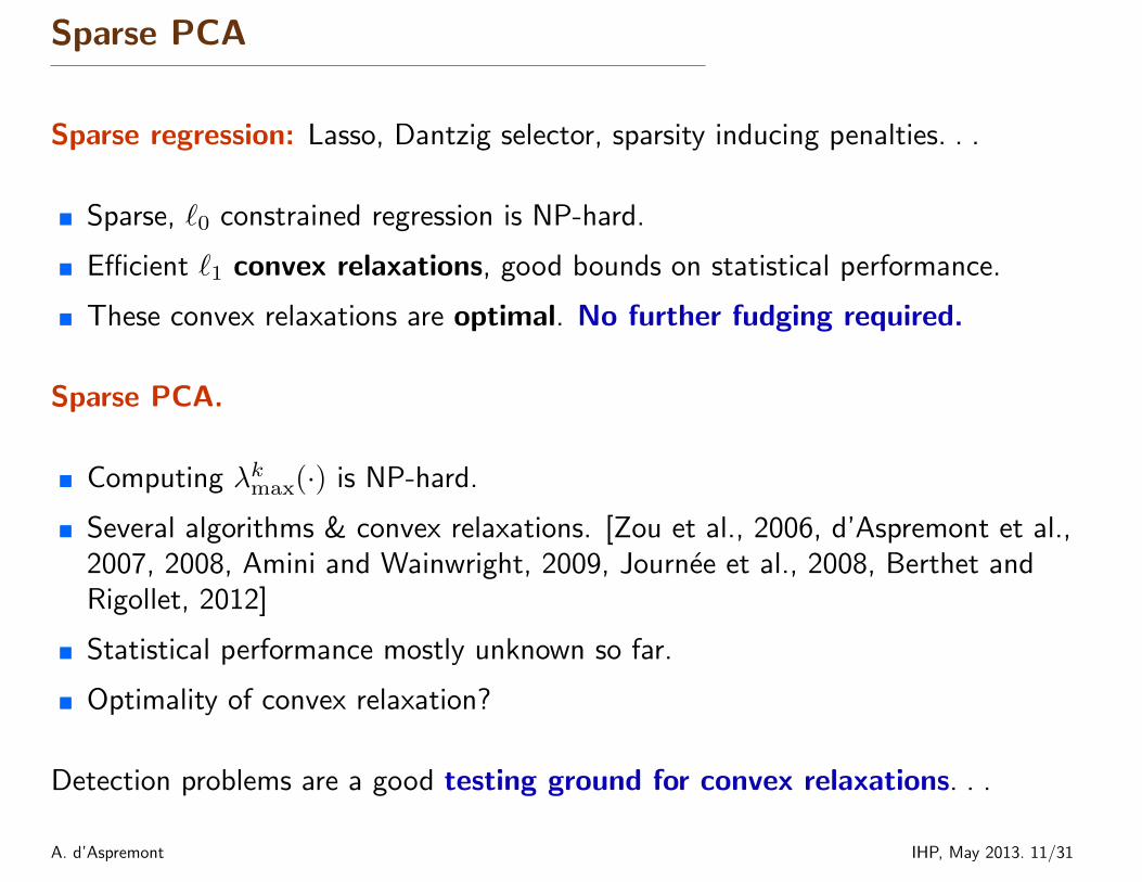
Sparse PCA

Sparse regression: Lasso, Dantzig selector, sparsity inducing penalties. . .

� Sparse, `0 constrained regression is NP-hard.

� Efficient `1 convex relaxations, good bounds on statistical performance.

� These convex relaxations are optimal. No further fudging required.

Sparse PCA.

� Computing λkmax(·) is NP-hard.

� Several algorithms & convex relaxations. [Zou et al., 2006, d’Aspremont et al.,2007, 2008, Amini and Wainwright, 2009, Journee et al., 2008, Berthet andRigollet, 2012]

� Statistical performance mostly unknown so far.

� Optimality of convex relaxation?

Detection problems are a good testing ground for convex relaxations. . .

A. d’Aspremont IHP, May 2013. 11/31

Outline

� PCA on high-dimensional data

� Approximation bounds for sparse eigenvalues

� Tractable detection for sparse PCA

� Algorithms

� Numerical results

A. d’Aspremont IHP, May 2013. 12/31

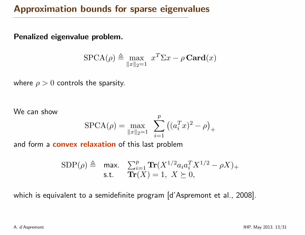
Approximation bounds for sparse eigenvalues

Penalized eigenvalue problem.

SPCA(ρ) , max‖x‖2=1

xTΣx− ρCard(x)

where ρ > 0 controls the sparsity.

We can show

SPCA(ρ) = max‖x‖2=1

p∑i=1

((aTi x)2 − ρ

)+

and form a convex relaxation of this last problem

SDP(ρ) , max.∑pi=1 Tr(X1/2aia

Ti X

1/2 − ρX)+

s.t. Tr(X) = 1, X � 0,

which is equivalent to a semidefinite program [d’Aspremont et al., 2008].

A. d’Aspremont IHP, May 2013. 13/31

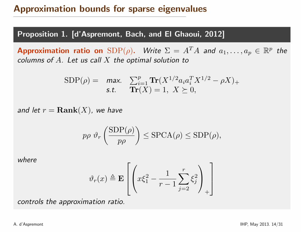
Approximation bounds for sparse eigenvalues

Proposition 1. [d’Aspremont, Bach, and El Ghaoui, 2012]

Approximation ratio on SDP(ρ). Write Σ = ATA and a1, . . . , ap ∈ Rp thecolumns of A. Let us call X the optimal solution to

SDP(ρ) = max.∑pi=1 Tr(X1/2aia

Ti X

1/2 − ρX)+

s.t. Tr(X) = 1, X � 0,

and let r = Rank(X), we have

pρ ϑr

(SDP(ρ)

pρ

)≤ SPCA(ρ) ≤ SDP(ρ),

where

ϑr(x) , E

xξ2

1 −1

r − 1

r∑j=2

ξ2j

+

controls the approximation ratio.

A. d’Aspremont IHP, May 2013. 14/31

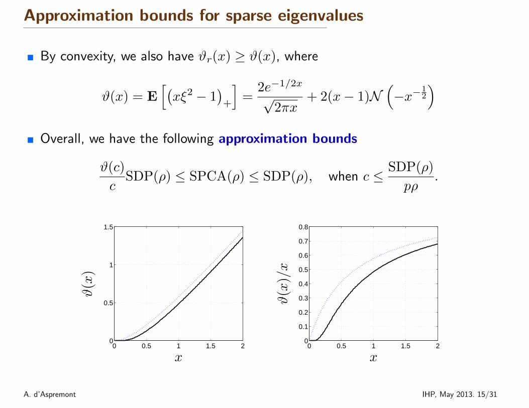
Approximation bounds for sparse eigenvalues

� By convexity, we also have ϑr(x) ≥ ϑ(x), where

ϑ(x) = E[(xξ2 − 1

)+

]=

2e−1/2x

√2πx

+ 2(x− 1)N(−x−1

2

)� Overall, we have the following approximation bounds

ϑ(c)

cSDP(ρ) ≤ SPCA(ρ) ≤ SDP(ρ), when c ≤ SDP(ρ)

pρ.

0 0.5 1 1.5 20

0.5

1

1.5

x

ϑ(x)

0 0.5 1 1.5 20

0.1

0.2

0.3

0.4

0.5

0.6

0.7

0.8

x

ϑ(x)/x

A. d’Aspremont IHP, May 2013. 15/31

Approximation bounds for sparse eigenvalues

Approximation ratio.

� No uniform approximation a la MAXCUT. . . But improved results for specificinstances, as in [Zwick, 1999] for MAXCUT on “heavy” cuts.

� Here, approximation quality is controlled by the ratio

SDP(ρ)

pρ

� Can we control this ratio for interesting problem instances?

A. d’Aspremont IHP, May 2013. 16/31

Outline

� PCA on high-dimensional data

� Approximation bounds for sparse eigenvalues

� Tractable detection for sparse PCA

� Algorithms

� Numerical results

A. d’Aspremont IHP, May 2013. 17/31

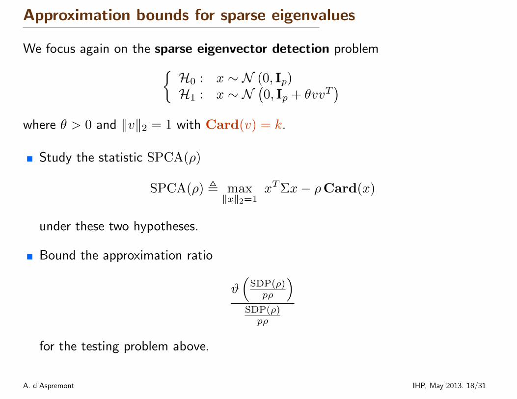
Approximation bounds for sparse eigenvalues

We focus again on the sparse eigenvector detection problem{H0 : x ∼ N (0, Ip)H1 : x ∼ N

(0, Ip + θvvT

)where θ > 0 and ‖v‖2 = 1 with Card(v) = k.

� Study the statistic SPCA(ρ)

SPCA(ρ) , max‖x‖2=1

xTΣx− ρCard(x)

under these two hypotheses.

� Bound the approximation ratio

ϑ(

SDP(ρ)pρ

)SDP(ρ)pρ

for the testing problem above.

A. d’Aspremont IHP, May 2013. 18/31

Approximation bounds for sparse eigenvalues

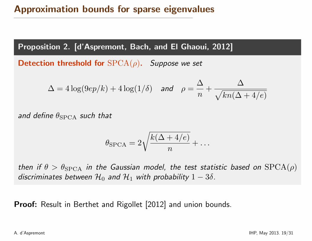
Proposition 2. [d’Aspremont, Bach, and El Ghaoui, 2012]

Detection threshold for SPCA(ρ). Suppose we set

∆ = 4 log(9ep/k) + 4 log(1/δ) and ρ =∆

n+

∆√kn(∆ + 4/e)

and define θSPCA such that

θSPCA = 2

√k(∆ + 4/e)

n+ . . .

then if θ > θSPCA in the Gaussian model, the test statistic based on SPCA(ρ)discriminates between H0 and H1 with probability 1− 3δ.

Proof: Result in Berthet and Rigollet [2012] and union bounds.

A. d’Aspremont IHP, May 2013. 19/31

Approximation bounds for sparse eigenvalues

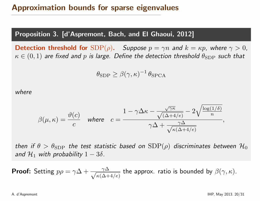
Proposition 3. [d’Aspremont, Bach, and El Ghaoui, 2012]

Detection threshold for SDP(ρ). Suppose p = γn and k = κp, where γ > 0,κ ∈ (0, 1) are fixed and p is large. Define the detection threshold θSDP such that

θSDP ≥ β(γ, κ)−1 θSPCA

where

β(µ, κ) =ϑ(c)

cwhere c =

1− γ∆κ−√γκ√

(∆+4/e)− 2√

log(1/δ)n

γ∆ + γ∆√κ(∆+4/e)

,

then if θ > θSDP the test statistic based on SDP(ρ) discriminates between H0

and H1 with probability 1− 3δ.

Proof: Setting pρ = γ∆ + γ∆√κ(∆+4/e)

the approx. ratio is bounded by β(γ, κ).

A. d’Aspremont IHP, May 2013. 20/31

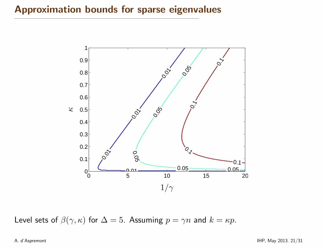
Approximation bounds for sparse eigenvalues

0.01

0.01

0.01

0.01 0.01 0.01

0.05

0.05

0.05

0.05 0.05

0.1

0.1

0.1

0.1

0 5 10 15 200

0.1

0.2

0.3

0.4

0.5

0.6

0.7

0.8

0.9

1

1/γ

κ

Level sets of β(γ, κ) for ∆ = 5. Assuming p = γn and k = κp.

A. d’Aspremont IHP, May 2013. 21/31

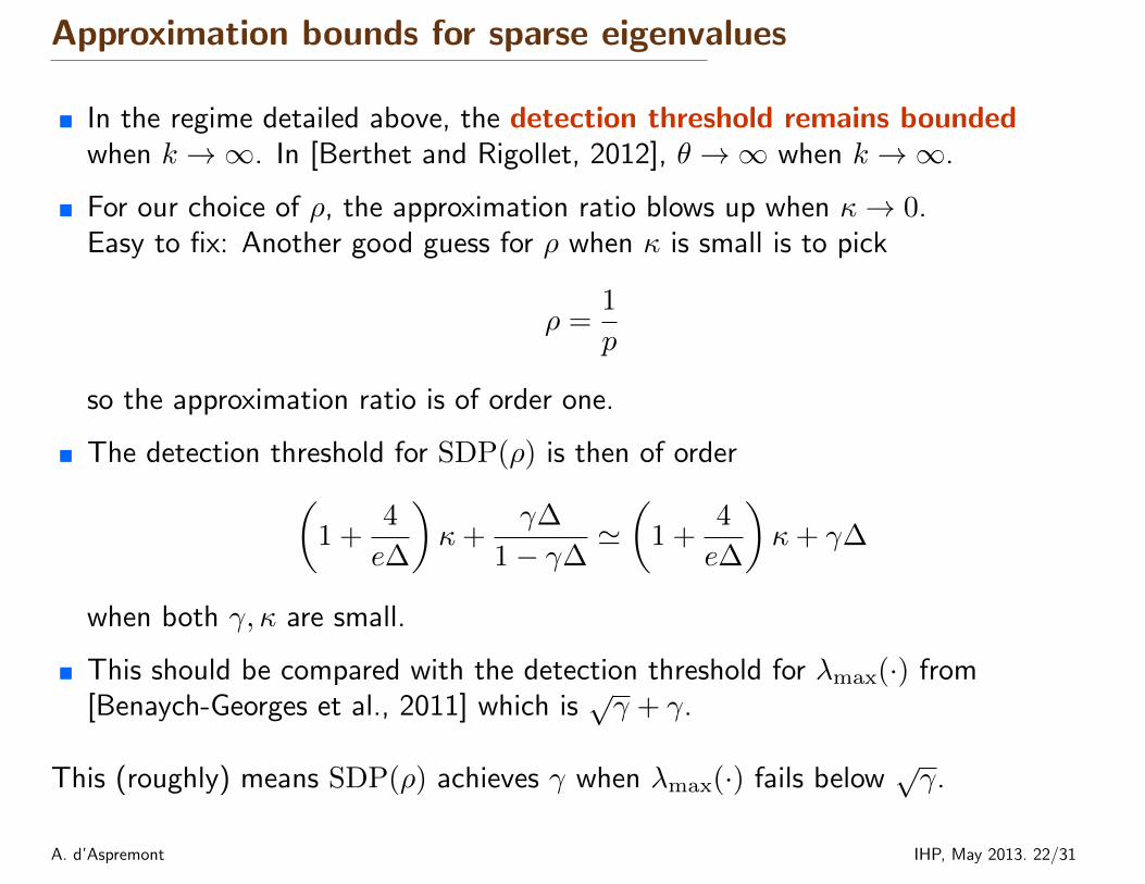
Approximation bounds for sparse eigenvalues

� In the regime detailed above, the detection threshold remains boundedwhen k →∞. In [Berthet and Rigollet, 2012], θ →∞ when k →∞.

� For our choice of ρ, the approximation ratio blows up when κ→ 0.Easy to fix: Another good guess for ρ when κ is small is to pick

ρ =1

p

so the approximation ratio is of order one.

� The detection threshold for SDP(ρ) is then of order(1 +

4

e∆

)κ+

γ∆

1− γ∆'(

1 +4

e∆

)κ+ γ∆

when both γ, κ are small.

� This should be compared with the detection threshold for λmax(·) from[Benaych-Georges et al., 2011] which is

√γ + γ.

This (roughly) means SDP(ρ) achieves γ when λmax(·) fails below√γ.

A. d’Aspremont IHP, May 2013. 22/31

Outline

� PCA on high-dimensional data

� Approximation bounds for sparse eigenvalues

� Tractable detection for sparse PCA

� Algorithms

� Numerical results

A. d’Aspremont IHP, May 2013. 23/31

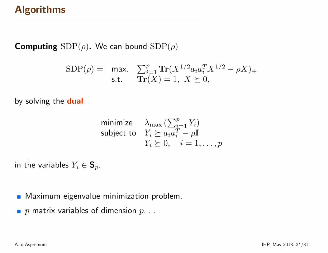
Algorithms

Computing SDP(ρ). We can bound SDP(ρ)

SDP(ρ) = max.∑pi=1 Tr(X1/2aia

Ti X

1/2 − ρX)+

s.t. Tr(X) = 1, X � 0,

by solving the dual

minimize λmax (∑pi=1 Yi)

subject to Yi � aiaTi − ρIYi � 0, i = 1, . . . , p

in the variables Yi ∈ Sp.

� Maximum eigenvalue minimization problem.

� p matrix variables of dimension p. . .

A. d’Aspremont IHP, May 2013. 24/31

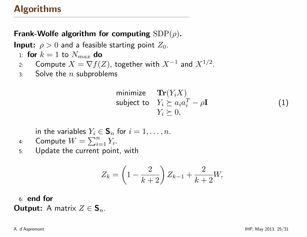
Algorithms

Frank-Wolfe algorithm for computing SDP(ρ).

Input: ρ > 0 and a feasible starting point Z0.1: for k = 1 to Nmax do2: Compute X = ∇f(Z), together with X−1 and X1/2.3: Solve the n subproblems

minimize Tr(YiX)subject to Yi � aiaTi − ρI

Yi � 0,(1)

in the variables Yi ∈ Sn for i = 1, . . . , n.4: Compute W =

∑ni=1 Yi.

5: Update the current point, with

Zk =

(1− 2

k + 2

)Zk−1 +

2

k + 2W,

6: end forOutput: A matrix Z ∈ Sn.

A. d’Aspremont IHP, May 2013. 25/31

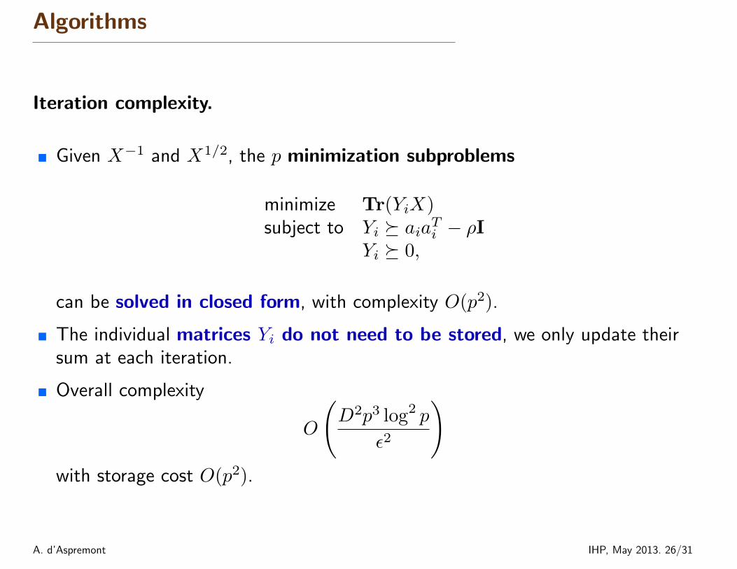
Algorithms

Iteration complexity.

� Given X−1 and X1/2, the p minimization subproblems

minimize Tr(YiX)subject to Yi � aiaTi − ρI

Yi � 0,

can be solved in closed form, with complexity O(p2).

� The individual matrices Yi do not need to be stored, we only update theirsum at each iteration.

� Overall complexity

O

(D2p3 log2 p

ε2

)with storage cost O(p2).

A. d’Aspremont IHP, May 2013. 26/31

Outline

� PCA on high-dimensional data

� Approximation bounds for sparse eigenvalues

� Tractable detection for sparse PCA

� Algorithms

� Numerical results

A. d’Aspremont IHP, May 2013. 27/31

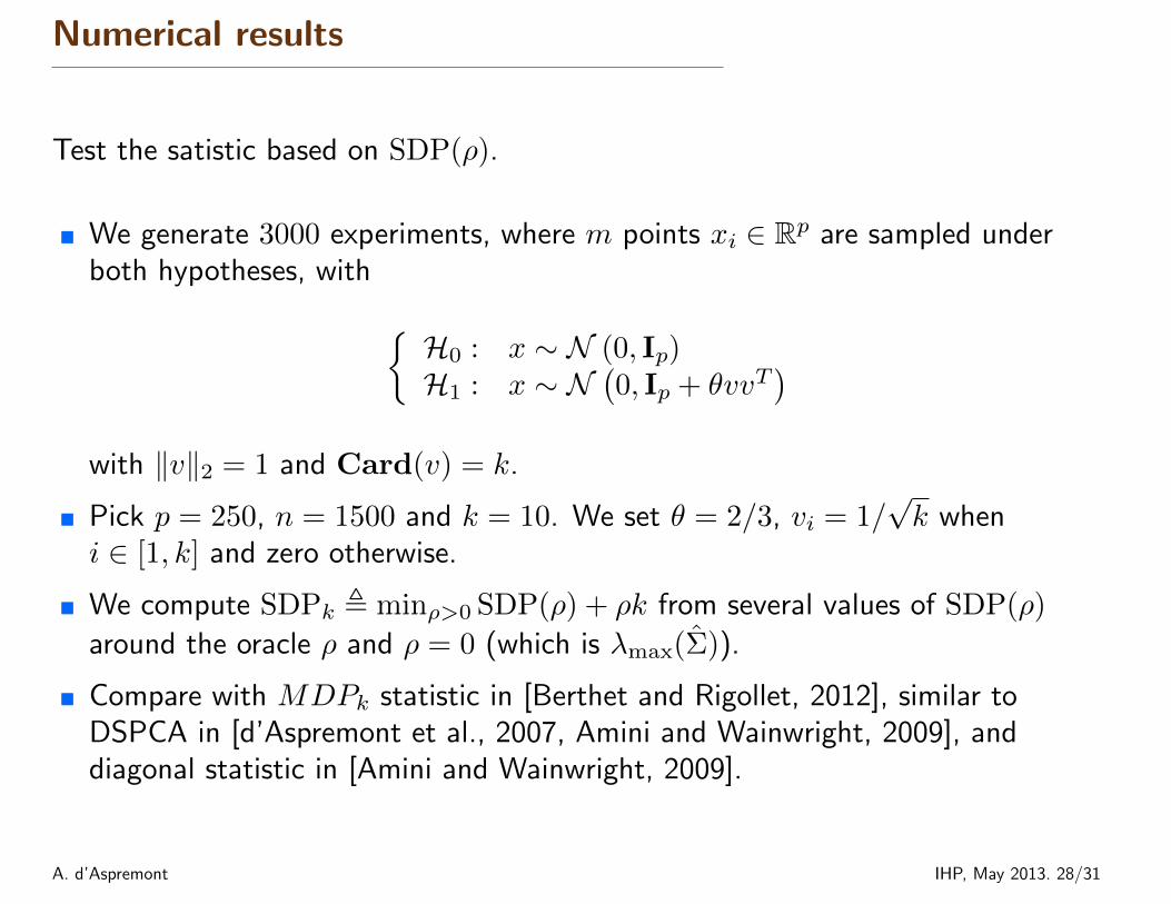
Numerical results

Test the satistic based on SDP(ρ).

� We generate 3000 experiments, where m points xi ∈ Rp are sampled underboth hypotheses, with {

H0 : x ∼ N (0, Ip)H1 : x ∼ N

(0, Ip + θvvT

)with ‖v‖2 = 1 and Card(v) = k.

� Pick p = 250, n = 1500 and k = 10. We set θ = 2/3, vi = 1/√k when

i ∈ [1, k] and zero otherwise.

� We compute SDPk , minρ>0 SDP(ρ) + ρk from several values of SDP(ρ)

around the oracle ρ and ρ = 0 (which is λmax(Σ)).

� Compare with MDPk statistic in [Berthet and Rigollet, 2012], similar toDSPCA in [d’Aspremont et al., 2007, Amini and Wainwright, 2009], anddiagonal statistic in [Amini and Wainwright, 2009].

A. d’Aspremont IHP, May 2013. 28/31

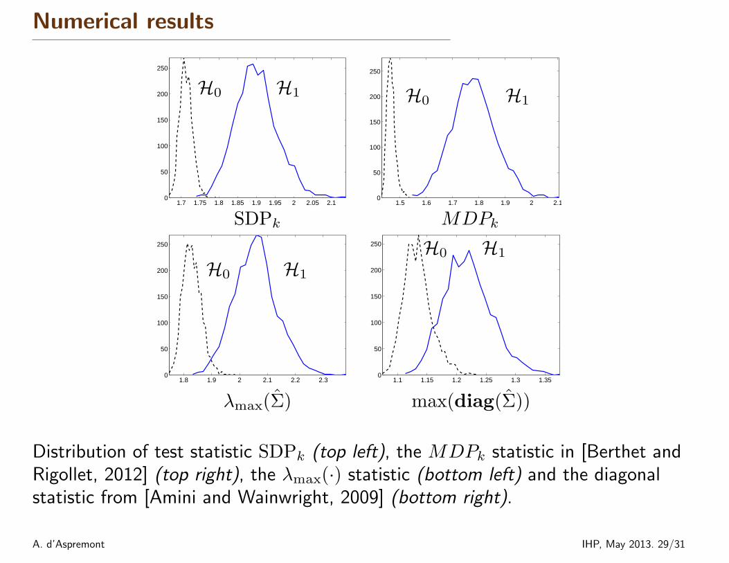
Numerical results

1.7 1.75 1.8 1.85 1.9 1.95 2 2.05 2.10

50

100

150

200

250

SDPk

H0 H1

1.5 1.6 1.7 1.8 1.9 2 2.10

50

100

150

200

250

MDPk

H0 H1

1.8 1.9 2 2.1 2.2 2.30

50

100

150

200

250

λmax(Σ)

H0 H1

1.1 1.15 1.2 1.25 1.3 1.350

50

100

150

200

250

max(diag(Σ))

H0 H1

Distribution of test statistic SDPk (top left), the MDPk statistic in [Berthet andRigollet, 2012] (top right), the λmax(·) statistic (bottom left) and the diagonalstatistic from [Amini and Wainwright, 2009] (bottom right).

A. d’Aspremont IHP, May 2013. 29/31

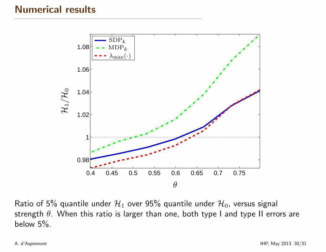
Numerical results

0.4 0.45 0.5 0.55 0.6 0.65 0.7 0.75

0.98

1

1.02

1.04

1.06

1.08

θ

H1/H

0

SDPk

MDPk

λmax(·)

Ratio of 5% quantile under H1 over 95% quantile under H0, versus signalstrength θ. When this ratio is larger than one, both type I and type II errors arebelow 5%.

A. d’Aspremont IHP, May 2013. 30/31

Conclusion

� Constant approximation bounds for sparse PCA relaxations in high dimensionalregimes.

� Explicit, finite bounds on detection threshold when p→∞.

Open questions. . . .

� More efficient SDP solver.

� Better approximation bounds for κ small? We should handle the case p >> n.

� Improved approximation ratio by direct analysis of the problem under H0?

� Model Selection: do we recover the correct sparse eigenvector? See [Aminiand Wainwright, 2009] for early results.

A. d’Aspremont IHP, May 2013. 31/31

*

References

A. Alon, N. Barkai, D. A. Notterman, K. Gish, S. Ybarra, D. Mack, and A. J. Levine. Broad patterns of gene expression revealed by clusteringanalysis of tumor and normal colon tissues probed by oligonucleotide arrays. Cell Biology, 96:6745–6750, 1999.

A.A. Amini and M. Wainwright. High-dimensional analysis of semidefinite relaxations for sparse principal components. The Annals ofStatistics, 37(5B):2877–2921, 2009.

J. Baik, G. Ben Arous, and S. Peche. Phase transition of the largest eigenvalue for nonnull complex sample covariance matrices. The Annalsof Probability, 33(5):1643–1697, 2005.

F. Benaych-Georges, A. Guionnet, and M. Maida. Fluctuations of the extreme eigenvalues of finite rank deformations of random matrices.Electron. J. Probab., 16:no. 60, 1621–1662, 2011. ISSN 1083-6489. doi: 10.1214/EJP.v16-929. URLhttp://dx.doi.org/10.1214/EJP.v16-929.

Q. Berthet and P. Rigollet. Optimal detection of sparse principal components in high dimension. Arxiv preprint arXiv:1202.5070, 2012.

A. d’Aspremont, L. El Ghaoui, M.I. Jordan, and G. R. G. Lanckriet. A direct formulation for sparse PCA using semidefinite programming.SIAM Review, 49(3):434–448, 2007.

A. d’Aspremont, F. Bach, and L. El Ghaoui. Optimal solutions for sparse principal component analysis. Journal of Machine LearningResearch, 9:1269–1294, 2008.

A. d’Aspremont, F. Bach, and L. El Ghaoui. Approximation bounds for sparse principal component analysis. ArXiv: 1205.0121, 2012.

S. Geman. A limit theorem for the norm of random matrices. The Annals of Probability, 8(2):252–261, 1980.

I.M. Johnstone. On the distribution of the largest eigenvalue in principal components analysis. Annals of Statistics, pages 295–327, 2001.

M. Journee, Y. Nesterov, P. Richtarik, and R. Sepulchre. Generalized power method for sparse principal component analysis. arXiv:0811.4724,2008.

N.E. Karoui. On the largest eigenvalue of wishart matrices with identity covariance when n, p and p/n tend to infinity. Arxiv preprintmath/0309355, 2003.

V.A. Marcenko and L.A. Pastur. Distribution of eigenvalues for some sets of random matrices. Mathematics of the USSR - Sbornik, 1(4):457–483, 1967.

T. Tao. Outliers in the spectrum of iid matrices with bounded rank perturbations. Probability Theory and Related Fields, pages 1–33, 2011.

YQ Yin, ZD Bai, and PR Krishnaiah. On the limit of the largest eigenvalue of the large dimensional sample covariance matrix. ProbabilityTheory and Related Fields, 78(4):509–521, 1988.

H. Zou, T. Hastie, and R. Tibshirani. Sparse Principal Component Analysis. Journal of Computational & Graphical Statistics, 15(2):265–286,2006.

A. d’Aspremont IHP, May 2013. 32/31

U. Zwick. Outward rotations: a tool for rounding solutions of semidefinite programming relaxations, with applications to max cut and otherproblems. In Proceedings of the thirty-first annual ACM symposium on Theory of computing, pages 679–687. ACM, 1999.

A. d’Aspremont IHP, May 2013. 33/31