Sudheer Siddapureddy

Department of Mechanical Engineering

sudheer@iitp.ac.in

Applied Thermodynamics - II

Gas Turbines – Shaft Power Real Cycles

Shaft Power Real Cycles Applied Thermodynamics - II

Real Cycles: Differ from Ideal Cycles

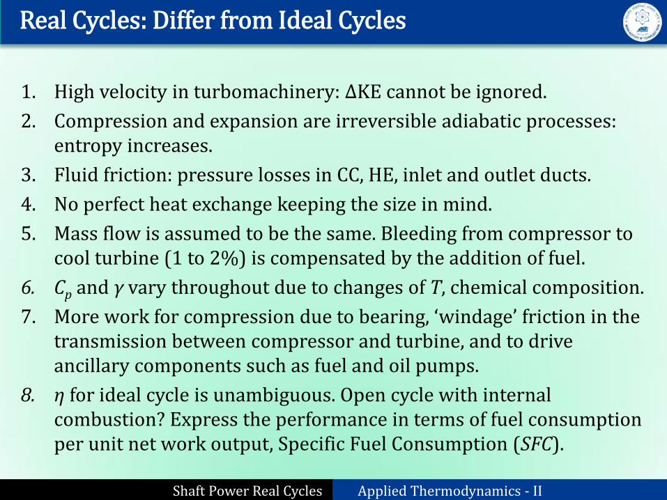
1. High velocity in turbomachinery: ΔKE cannot be ignored.

2. Compression and expansion are irreversible adiabatic processes: entropy increases.

3. Fluid friction: pressure losses in CC, HE, inlet and outlet ducts.

4. No perfect heat exchange keeping the size in mind.

5. Mass flow is assumed to be the same. Bleeding from compressor to cool turbine (1 to 2%) is compensated by the addition of fuel.

6. Cp and γ vary throughout due to changes of T, chemical composition.

7. More work for compression due to bearing, ‘windage’ friction in the transmission between compressor and turbine, and to drive ancillary components such as fuel and oil pumps.

8. η for ideal cycle is unambiguous. Open cycle with internal combustion? Express the performance in terms of fuel consumption per unit net work output, Specific Fuel Consumption (SFC).

Shaft Power Real Cycles Applied Thermodynamics - II

1. Change in Fluid Velocity

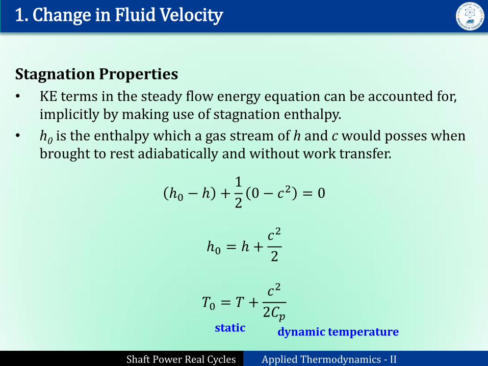
Stagnation Properties

• KE terms in the steady flow energy equation can be accounted for, implicitly by making use of stagnation enthalpy.

• h0 is the enthalpy which a gas stream of h and c would posses when brought to rest adiabatically and without work transfer.

ℎ0 − ℎ +1

20 − 𝑐2 = 0

ℎ0 = ℎ +𝑐2

2

𝑇0 = 𝑇 +𝑐2

2𝐶𝑝

static dynamic temperature

Shaft Power Real Cycles Applied Thermodynamics - II

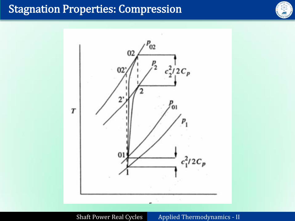
Stagnation Properties: Compression

Shaft Power Real Cycles Applied Thermodynamics - II

1. Change in Fluid Velocity

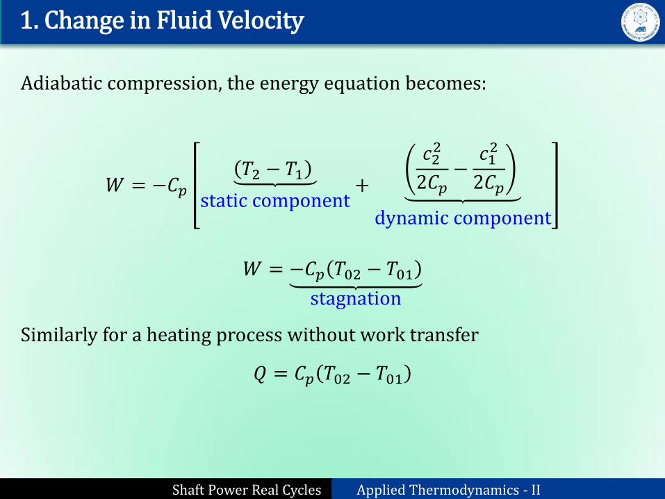
Adiabatic compression, the energy equation becomes:

𝑊 = −𝐶𝑝𝑇2 − 𝑇1

static component+

𝑐22

2𝐶𝑝−

𝑐12

2𝐶𝑝

dynamic component

𝑊 = −𝐶𝑝 𝑇02 − 𝑇01

stagnation

Similarly for a heating process without work transfer

𝑄 = 𝐶𝑝 𝑇02 − 𝑇01

Shaft Power Real Cycles Applied Thermodynamics - II

1. Change in Fluid Velocity

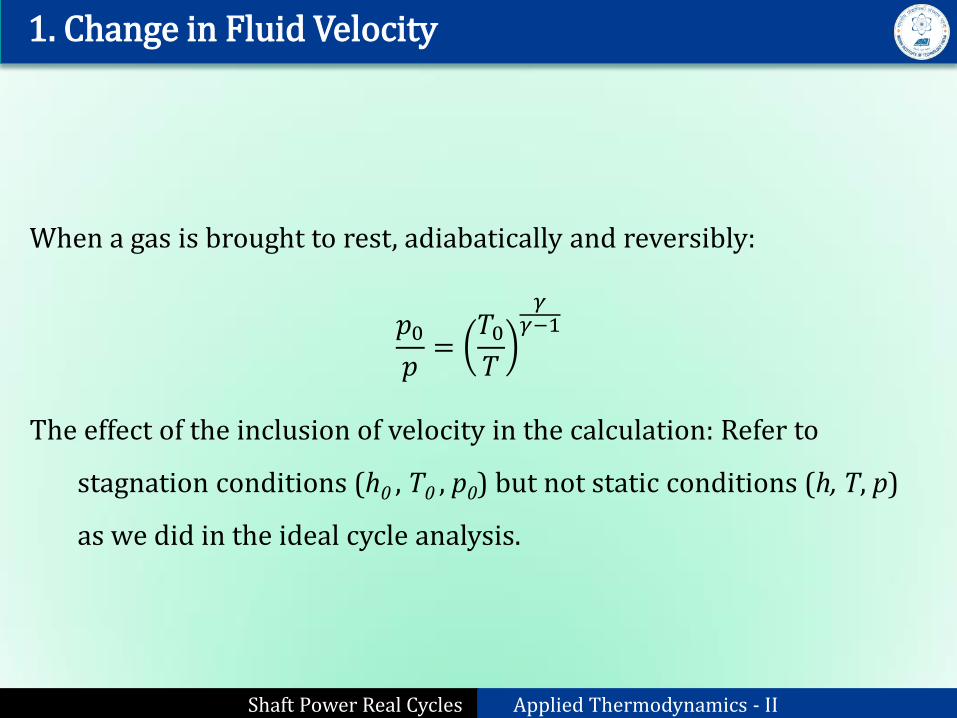
When a gas is brought to rest, adiabatically and reversibly:

𝑝0𝑝=

𝑇0𝑇

𝛾𝛾−1

The effect of the inclusion of velocity in the calculation: Refer to

stagnation conditions (h0 , T0 , p0) but not static conditions (h, T, p)

as we did in the ideal cycle analysis.

Shaft Power Real Cycles Applied Thermodynamics - II

Real Cycles: Differ from Ideal Cycles

1. High velocity in turbomachinery: ΔKE cannot be ignored.

2. Compression and expansion are irreversible adiabatic processes: entropy increases.

3. Fluid friction: pressure losses in CC, HE, inlet and outlet ducts.

4. No perfect heat exchange keeping the size in mind.

5. Mass flow is assumed to be the same. Bleeding from compressor to cool turbine (1 to 2%) is compensated by the addition of fuel.

6. Cp and γ vary throughout due to changes of T, chemical composition.

7. More work for compression due to bearing, ‘windage’ friction in the transmission between compressor and turbine, and to drive ancillary components such as fuel and oil pumps.

8. η for ideal cycle is unambiguous. Open cycle with internal combustion? Express the performance in terms of fuel consumption per unit net work output, Specific Fuel Consumption (SFC).

Shaft Power Real Cycles Applied Thermodynamics - II

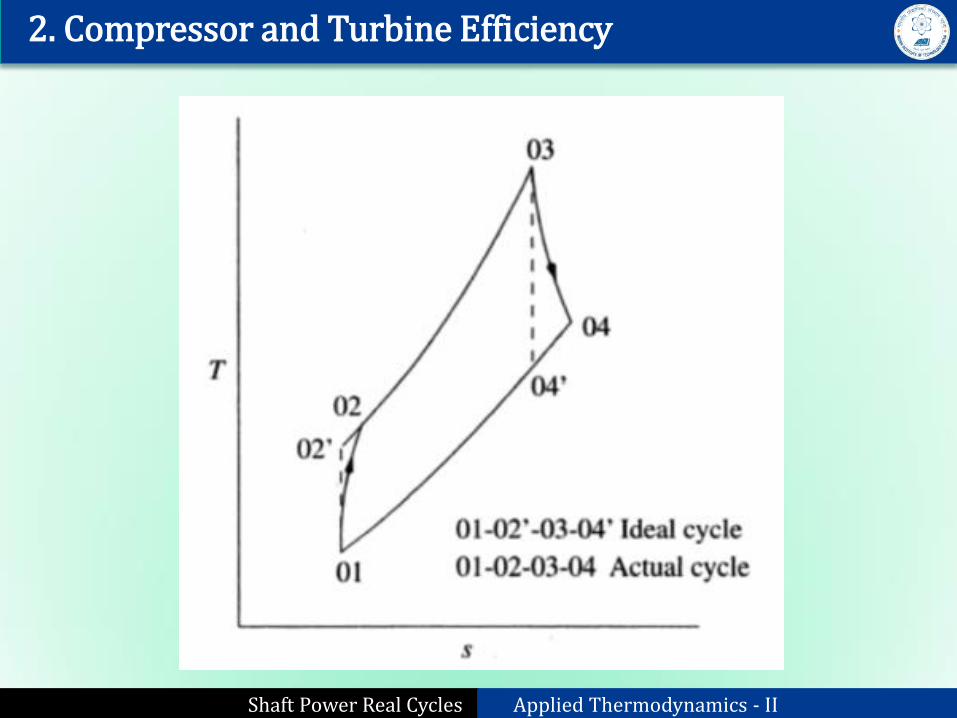
2. Compressor and Turbine Efficiency

Shaft Power Real Cycles Applied Thermodynamics - II

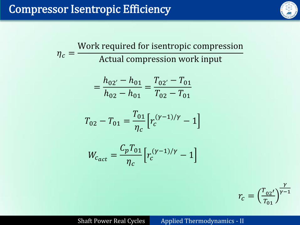
Compressor Isentropic Efficiency

𝜂𝑐 =Work required for isentropic compression

Actual compression work input

=ℎ02′ − ℎ01ℎ02 − ℎ01

=𝑇02′ − 𝑇01𝑇02 − 𝑇01

𝑇02 − 𝑇01 =𝑇01𝜂𝑐

𝑟𝑐(𝛾−1)/𝛾

− 1

𝑊𝑐𝑎𝑐𝑡 =𝐶𝑝𝑇01

𝜂𝑐𝑟𝑐(𝛾−1)/𝛾

− 1

𝑟𝑐 =𝑇02′

𝑇01

𝛾

𝛾−1

Shaft Power Real Cycles Applied Thermodynamics - II

Turbine Isentropic Efficiency

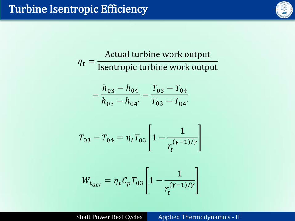
𝜂𝑡 =Actual turbine work output

Isentropic turbine work output

=ℎ03 − ℎ04ℎ03 − ℎ04′

=𝑇03 − 𝑇04𝑇03 − 𝑇04′

𝑇03 − 𝑇04 = 𝜂𝑡𝑇03 1 −1

𝑟𝑡(𝛾−1)/𝛾

𝑊𝑡𝑎𝑐𝑡 = 𝜂𝑡𝐶𝑝𝑇03 1 −1

𝑟𝑡(𝛾−1)/𝛾

Shaft Power Real Cycles Applied Thermodynamics - II

3. Pressure or Flow Losses

Losses due to friction & turbulence occurs throughout the whole plant.

1. Air side intercooler loss

2. Air side heat exchanger loss

3. Combustion chamber loss (both main and reheat)

4. Gas side heat exchanger loss

5. Duct losses between components and at intake and exhaust

The pressure losses have the effect of decreasing rt relative to rc

Reduces net work output from the plant

Gas turbine cycle is very sensitive to irreversibilities:

Δp significantly effects the cycle performance

Shaft Power Real Cycles Applied Thermodynamics - II

Pressure or Flow Losses

Shaft Power Real Cycles Applied Thermodynamics - II

Pressure or Flow Losses

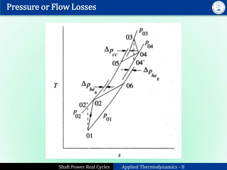
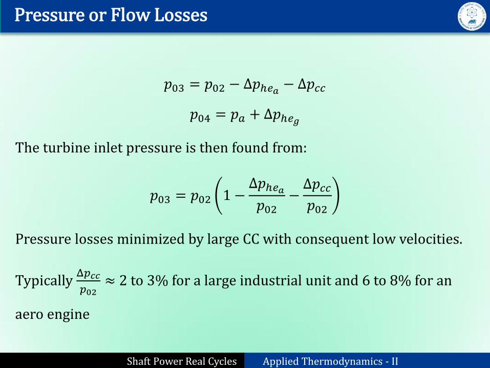
𝑝03 = 𝑝02 − ∆𝑝ℎ𝑒𝑎 − ∆𝑝𝑐𝑐

𝑝04 = 𝑝𝑎 + ∆𝑝ℎ𝑒𝑔

The turbine inlet pressure is then found from:

𝑝03 = 𝑝02 1 −Δ𝑝ℎ𝑒𝑎𝑝02

−Δ𝑝𝑐𝑐𝑝02

Pressure losses minimized by large CC with consequent low velocities.

Typically Δ𝑝𝑐𝑐

𝑝02≈ 2 to 3% for a large industrial unit and 6 to 8% for an

aero engine

Shaft Power Real Cycles Applied Thermodynamics - II

4. Heat Exchanger Effectiveness

Shaft Power Real Cycles Applied Thermodynamics - II

4. Heat Exchanger Effectiveness

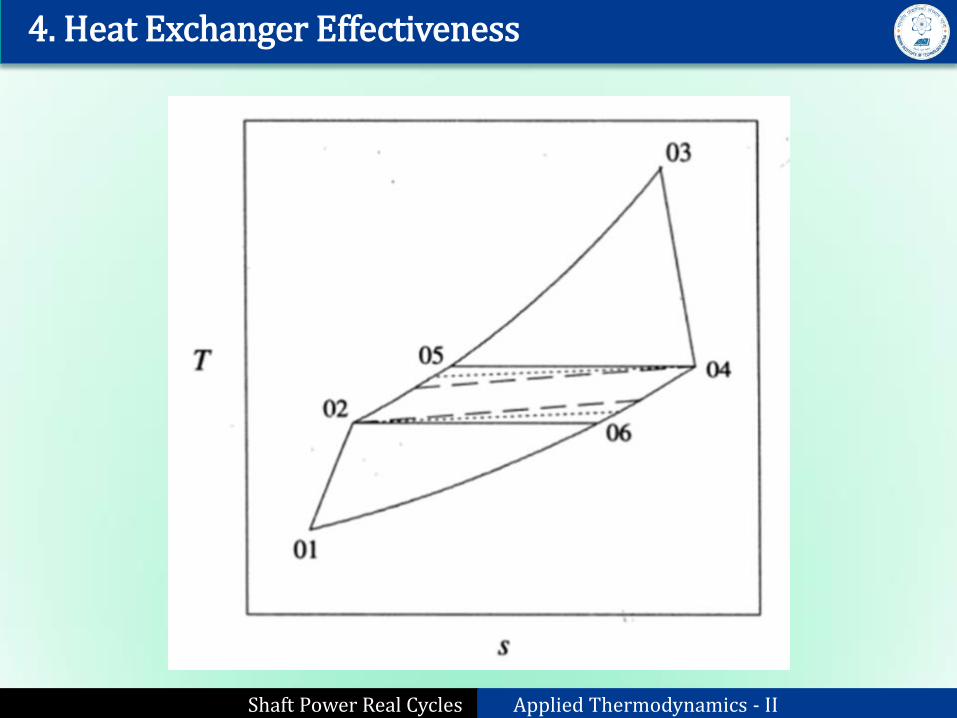
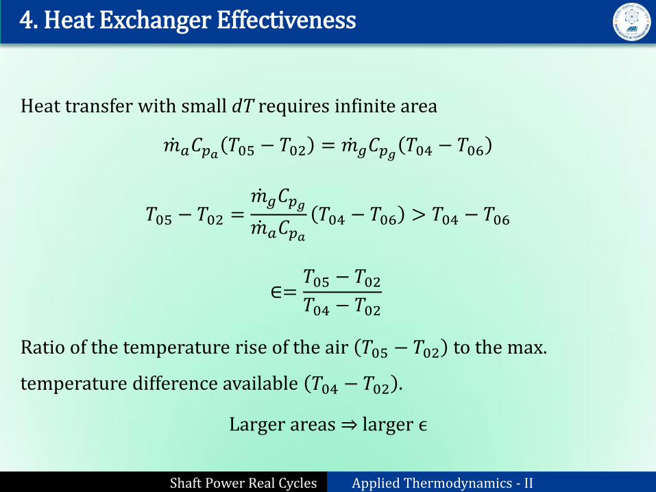
Heat transfer with small dT requires infinite area

𝑚 𝑎𝐶𝑝𝑎 𝑇05 − 𝑇02 = 𝑚 𝑔𝐶𝑝𝑔 𝑇04 − 𝑇06

𝑇05 − 𝑇02 =𝑚 𝑔𝐶𝑝𝑔𝑚 𝑎𝐶𝑝𝑎

𝑇04 − 𝑇06 > 𝑇04 − 𝑇06

∈=𝑇05 − 𝑇02𝑇04 − 𝑇02

Ratio of the temperature rise of the air 𝑇05 − 𝑇02 to the max.

temperature difference available 𝑇04 − 𝑇02 .

Larger areas ⇒ larger ϵ

Shaft Power Real Cycles Applied Thermodynamics - II

5. Effect of Varying Mass Flow

𝑚 𝑔 = 𝑚 𝑎 +𝑚 𝑓

𝑚 𝑔

𝑚 𝑎= 1 +

𝑚 𝑓

𝑚 𝑎= 1 + 𝑓

However, this increase is compensated by the bleeding compressed air

to turbine cooling.

Overall air-fuel ratio of the order of 60:1 to 100:1.

Shaft Power Real Cycles Applied Thermodynamics - II

6. Effect of Variable Specific Heat

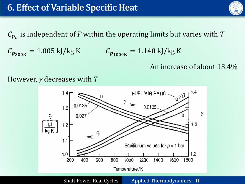
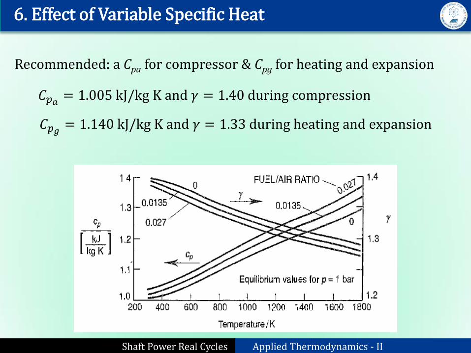
𝐶𝑝𝑎 is independent of P within the operating limits but varies with T

𝐶𝑝300K = 1.005 kJ/kg K 𝐶𝑝1000K = 1.140 kJ/kg K

An increase of about 13.4%

However, γ decreases with T

Shaft Power Real Cycles Applied Thermodynamics - II

6. Effect of Variable Specific Heat

Recommended: a Cpa for compressor & Cpg for heating and expansion

𝐶𝑝𝑎 = 1.005 kJ/kg K and 𝛾 = 1.40 during compression

𝐶𝑝𝑔 = 1.140 kJ/kg K and 𝛾 = 1.33 during heating and expansion

Shaft Power Real Cycles Applied Thermodynamics - II

7. Mechanical Losses

Bearing friction, windage amounts to 10% of compressor work (Wc)

𝑊𝑐 =1

𝜂𝑚𝑒𝑐ℎ𝐶𝑝𝑎 𝑇02 − 𝑇01

Shaft Power Real Cycles Applied Thermodynamics - II

8. Loss due to Incomplete Combustion

𝜂𝑏 =Enthalpy released

Available entalpy of fuel= 0.98

Shaft Power Real Cycles Applied Thermodynamics - II

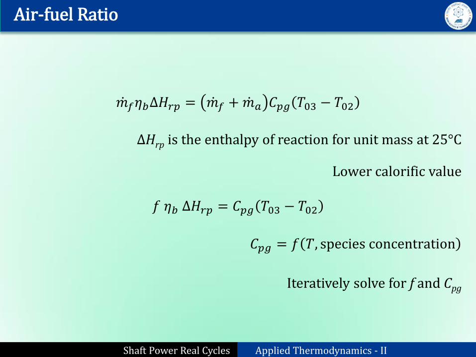
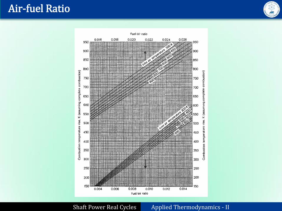
Air-fuel Ratio

𝑚 𝑓𝜂𝑏∆𝐻𝑟𝑝 = 𝑚 𝑓 +𝑚 𝑎 𝐶𝑝𝑔 𝑇03 − 𝑇02

ΔHrp is the enthalpy of reaction for unit mass at 25°C

Lower calorific value

𝑓 𝜂𝑏 ∆𝐻𝑟𝑝 = 𝐶𝑝𝑔 𝑇03 − 𝑇02

𝐶𝑝𝑔 = 𝑓 𝑇, species concentration

Iteratively solve for f and Cpg

Shaft Power Real Cycles Applied Thermodynamics - II

Air-fuel Ratio

Shaft Power Real Cycles Applied Thermodynamics - II

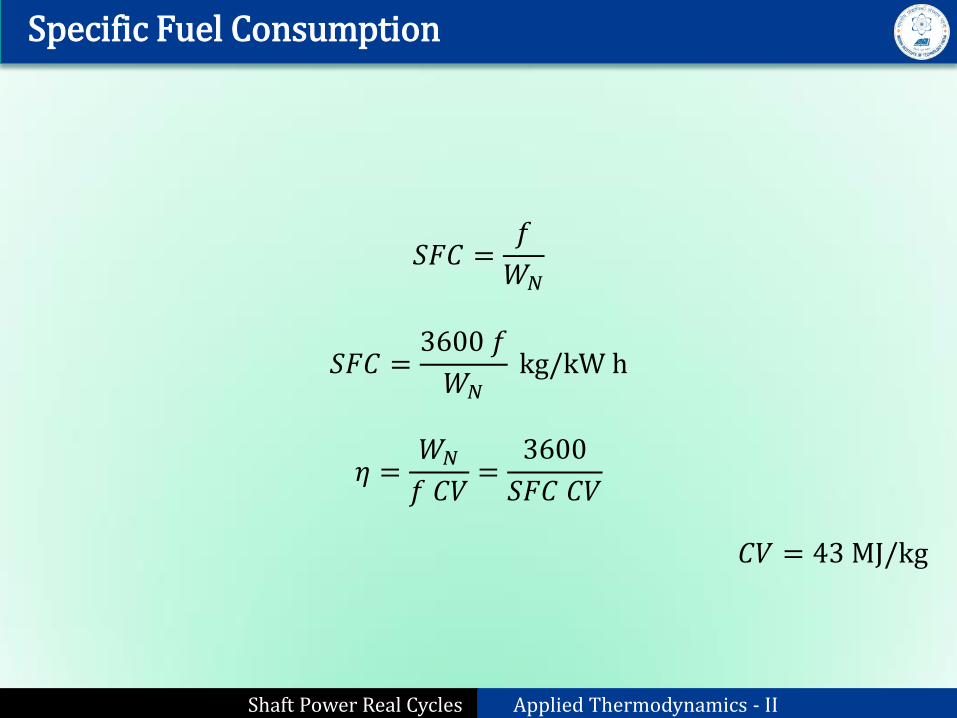
Specific Fuel Consumption

𝑆𝐹𝐶 =𝑓

𝑊𝑁

𝑆𝐹𝐶 =3600 𝑓

𝑊𝑁 kg/kW h

𝜂 =𝑊𝑁

𝑓 𝐶𝑉=

3600

𝑆𝐹𝐶 𝐶𝑉

𝐶𝑉 = 43 MJ/kg

Shaft Power Real Cycles Applied Thermodynamics - II

Polytropic Efficiency

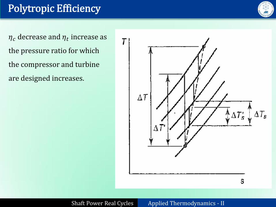
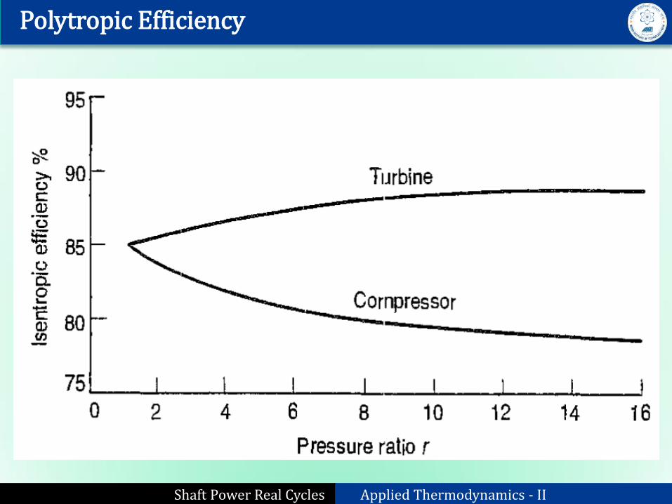
𝜂𝑐 decrease and 𝜂𝑡 increase as

the pressure ratio for which

the compressor and turbine

are designed increases.

Shaft Power Real Cycles Applied Thermodynamics - II

Polytropic Efficiency

𝜂𝑠𝜂𝑐

=∑Δ𝑇𝑠

′

Δ𝑇′

• 𝜂𝑠 > 𝜂𝑐 and this difference increases with number of stages (r).

• Meaning work is required due to ‘preheat’ effect.

• Similarly for a turbine 𝜂𝑡 > 𝜂𝑠. Frictional ‘reheating’ in one stage is partially recovered as work in the next.

• Polytropic efficiency is the isentropic efficiency of an elemental stage in the process such that it is constant throughout the whole process.

𝜂𝑠𝑐 =𝑑𝑇′

𝑑𝑇= constant

𝑇

𝑝(𝛾−1)/𝛾= constant

Shaft Power Real Cycles Applied Thermodynamics - II

Polytropic Efficiency

𝑑𝑇′

𝑇=𝛾 − 1

𝛾

𝑑𝑝

𝑝

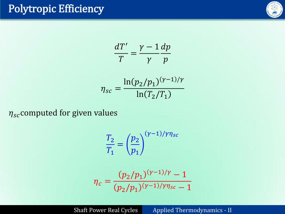
𝜂𝑠𝑐 =ln 𝑝2/𝑝1

𝛾−1 /𝛾

ln 𝑇2/𝑇1

𝜂𝑠𝑐computed for given values

𝑇2𝑇1

=𝑝2𝑝1

𝛾−1 /𝛾𝜂𝑠𝑐

𝜂𝑐 =𝑝2/𝑝1

𝛾−1 /𝛾 − 1

𝑝2/𝑝1𝛾−1 /𝛾𝜂𝑠𝑐 − 1

Shaft Power Real Cycles Applied Thermodynamics - II

Polytropic Efficiency

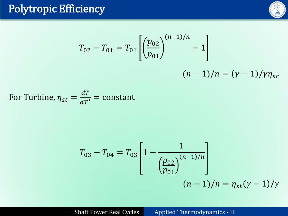
𝑇02 − 𝑇01 = 𝑇01𝑝02𝑝01

𝑛−1 /𝑛

− 1

(𝑛 − 1)/𝑛 = 𝛾 − 1 /𝛾𝜂𝑠𝑐

For Turbine, 𝜂𝑠𝑡 =𝑑𝑇

𝑑𝑇′= constant

𝑇03 − 𝑇04 = 𝑇03 1 −1

𝑝02𝑝01

𝑛−1 /𝑛

(𝑛 − 1)/𝑛 = 𝜂𝑠𝑡 𝛾 − 1 /𝛾

Shaft Power Real Cycles Applied Thermodynamics - II

Polytropic Efficiency

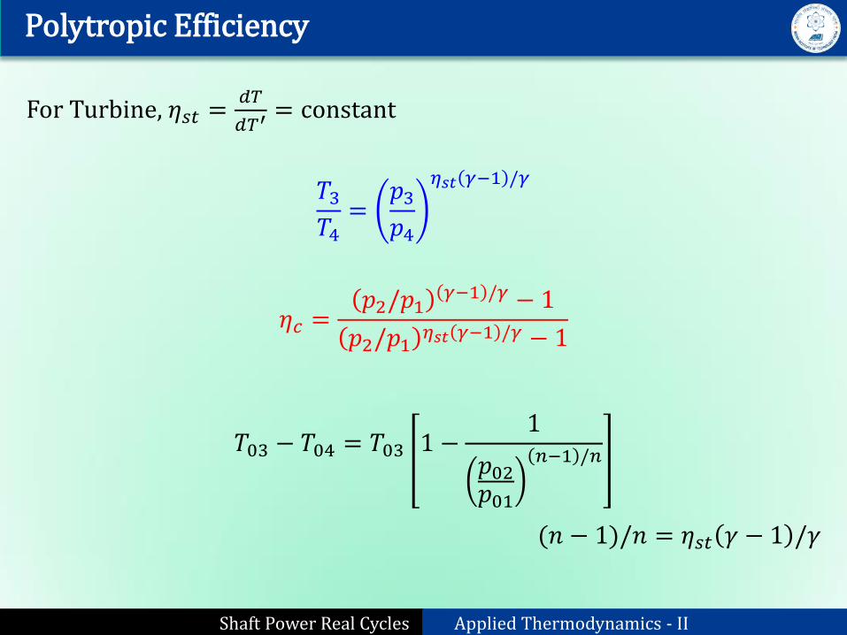
For Turbine, 𝜂𝑠𝑡 =𝑑𝑇

𝑑𝑇′= constant

𝑇3𝑇4

=𝑝3𝑝4

𝜂𝑠𝑡 𝛾−1 /𝛾

𝜂𝑐 =𝑝2/𝑝1

𝛾−1 /𝛾 − 1

𝑝2/𝑝1𝜂𝑠𝑡 𝛾−1 /𝛾 − 1

𝑇03 − 𝑇04 = 𝑇03 1 −1

𝑝02𝑝01

𝑛−1 /𝑛

(𝑛 − 1)/𝑛 = 𝜂𝑠𝑡 𝛾 − 1 /𝛾

Shaft Power Real Cycles Applied Thermodynamics - II

Polytropic Efficiency

Shaft Power Real Cycles Applied Thermodynamics - II

Problem: Real Cycle Analysis

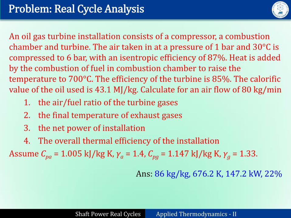
An oil gas turbine installation consists of a compressor, a combustion chamber and turbine. The air taken in at a pressure of 1 bar and 30°C is compressed to 6 bar, with an isentropic efficiency of 87%. Heat is added by the combustion of fuel in combustion chamber to raise the temperature to 700°C. The efficiency of the turbine is 85%. The calorific value of the oil used is 43.1 MJ/kg. Calculate for an air flow of 80 kg/min

1. the air/fuel ratio of the turbine gases

2. the final temperature of exhaust gases

3. the net power of installation

4. The overall thermal efficiency of the installation

Assume Cpa = 1.005 kJ/kg K, γa = 1.4, Cpg = 1.147 kJ/kg K, γg = 1.33.

Ans: 86 kg/kg, 676.2 K, 147.2 kW, 22%

Shaft Power Real Cycles Applied Thermodynamics - II

Problem: Real Cycle Analysis

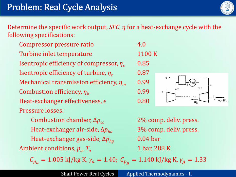
Determine the specific work output, SFC, η for a heat-exchange cycle with the following specifications:

Compressor pressure ratio 4.0

Turbine inlet temperature 1100 K

Isentropic efficiency of compressor, ηc 0.85

Isentropic efficiency of turbine, ηt 0.87

Mechanical transmission efficiency, ηm 0.99

Combustion efficiency, ηb 0.99

Heat-exchanger effectiveness, ϵ 0.80

Pressure losses:

Combustion chamber, Δpcc 2% comp. deliv. press.

Heat-exchanger air-side, Δpha 3% comp. deliv. press.

Heat-exchanger gas-side, Δphg 0.04 bar

Ambient conditions, pa, Ta 1 bar, 288 K

𝐶𝑝𝑎 = 1.005 kJ/kg K, 𝛾𝑎 = 1.40; 𝐶𝑝𝑔 = 1.140 kJ/kg K, 𝛾𝑔 = 1.33

Shaft Power Real Cycles Applied Thermodynamics - II

Problem: Real Cycle Analysis

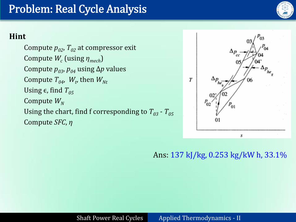
Hint

Compute p02, T02 at compressor exit

Compute Wc (using ηmech)

Compute p03, p04 using Δp values

Compute T04, Wt, then WNt

Using ϵ, find T05

Compute WN

Using the chart, find f corresponding to T03 - T05

Compute SFC, η

Ans: 137 kJ/kg, 0.253 kg/kW h, 33.1%

Shaft Power Real Cycles Applied Thermodynamics - II

Problem: Real Cycle Analysis

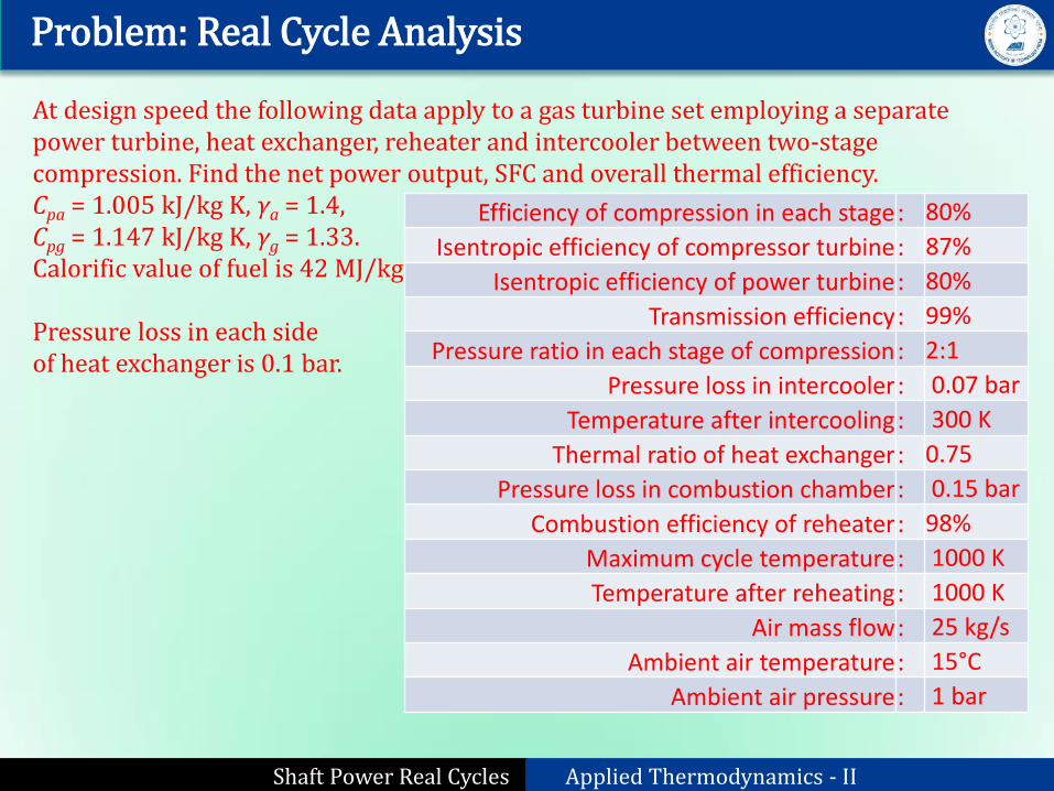
At design speed the following data apply to a gas turbine set employing a separate power turbine, heat exchanger, reheater and intercooler between two-stage compression. Find the net power output, SFC and overall thermal efficiency. Cpa = 1.005 kJ/kg K, γa = 1.4, Cpg = 1.147 kJ/kg K, γg = 1.33. Calorific value of fuel is 42 MJ/kg Pressure loss in each side of heat exchanger is 0.1 bar.

Efficiency of compression in each stage : 80%

Isentropic efficiency of compressor turbine : 87%

Isentropic efficiency of power turbine : 80%

Transmission efficiency : 99%

Pressure ratio in each stage of compression : 2:1

Pressure loss in intercooler : 0.07 bar

Temperature after intercooling : 300 K

Thermal ratio of heat exchanger : 0.75

Pressure loss in combustion chamber : 0.15 bar

Combustion efficiency of reheater : 98%

Maximum cycle temperature : 1000 K

Temperature after reheating : 1000 K

Air mass flow : 25 kg/s

Ambient air temperature : 15°C

Ambient air pressure : 1 bar