6. Laminar and turbulent boundary layers

John Richard Thome

8 avril 2008

John Richard Thome (LTCM - SGM - EPFL) Heat transfer - Convection 8 avril 2008 1 / 34

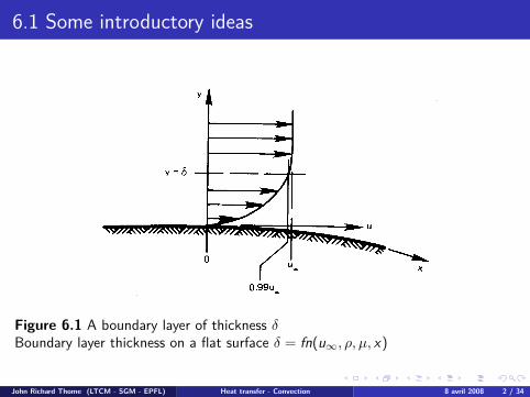
6.1 Some introductory ideas

Figure 6.1 A boundary layer of thickness δBoundary layer thickness on a flat surface δ = fn(u∞, ρ, µ, x)

John Richard Thome (LTCM - SGM - EPFL) Heat transfer - Convection 8 avril 2008 2 / 34

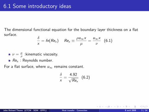
6.1 Some introductory ideas

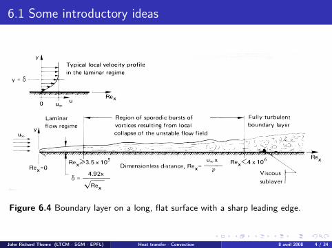
The dimensional functional equation for the boundary layer thickness on a flatsurface.

δ

x = fn(Rex ) Rex ≡ρu∞xµ

=u∞xν

(6.1)

ν = µρ :kinematic viscosity.

Rex : Reynolds number.For a flat surface, where u∞ remains constant.

δ

x =4.92√Rex

(6.2)

John Richard Thome (LTCM - SGM - EPFL) Heat transfer - Convection 8 avril 2008 3 / 34

6.1 Some introductory ideas

Figure 6.4 Boundary layer on a long, flat surface with a sharp leading edge.

John Richard Thome (LTCM - SGM - EPFL) Heat transfer - Convection 8 avril 2008 4 / 34

6.1 Some introductory ideas

(uav )crit : Transitional value of the average velocity.

Recritical ≡ρD(uav )crit

µ(6.3)

Rexcritical =u∞xcritν

(6.4)

Transition from laminar to turbulent flow.

Rex ,c = 5 · 105

John Richard Thome (LTCM - SGM - EPFL) Heat transfer - Convection 8 avril 2008 5 / 34

Thermal boundary layer

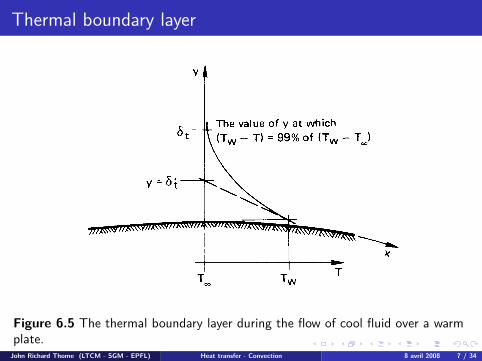
The wall is at temperature Tw

−kf (∂T∂y |y=0) = (Tw − T∞)h (6.5)

Where kf is the conductivity of the fluid. The following condition defined h withinthe fluid instead of specifying it as known information on the boundary.

∂(

Tw−TTw−T∞

)∂( y

L) | y

L =0 =hLkf

= NuL (6.5a)

The physical significance of Nu is given by

NuL =≡ hxkf

=Lδ′t

(6.6)

The nusselt number is inversely proportional to the thickness of the thermalboundary layer δ′t .

John Richard Thome (LTCM - SGM - EPFL) Heat transfer - Convection 8 avril 2008 6 / 34

Thermal boundary layer

Figure 6.5 The thermal boundary layer during the flow of cool fluid over a warmplate.John Richard Thome (LTCM - SGM - EPFL) Heat transfer - Convection 8 avril 2008 7 / 34

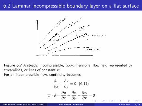
6.2 Laminar incompressible boundary layer on a flat surface

Figure 6.7 A steady, incompressible, two-dimensional flow field represented bystreamlines, or lines of constant ψ.For an incompressible flow, continuity becomes

∂u∂x +

∂v∂y = 0 (6.11)

5 · ~u =∂u∂x +

∂v∂y +

∂w∂z = 0

John Richard Thome (LTCM - SGM - EPFL) Heat transfer - Convection 8 avril 2008 8 / 34

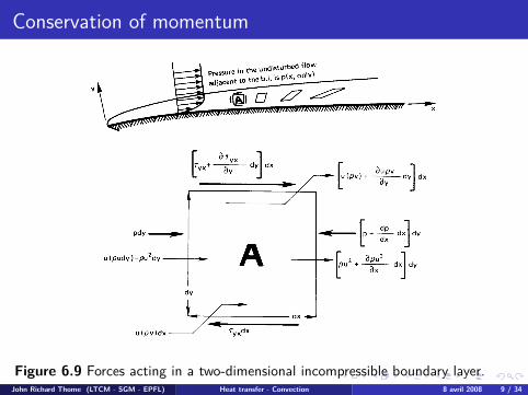
Conservation of momentum

Figure 6.9 Forces acting in a two-dimensional incompressible boundary layer.John Richard Thome (LTCM - SGM - EPFL) Heat transfer - Convection 8 avril 2008 9 / 34

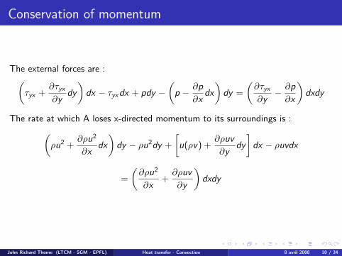
Conservation of momentum

The external forces are :(τyx +

∂τyx∂y dy

)dx − τyxdx + pdy −

(p − ∂p

∂x dx)dy =

(∂τyx∂y −

∂p∂x

)dxdy

The rate at which A loses x-directed momentum to its surroundings is :(ρu2 +

∂ρu2

∂x dx)dy − ρu2dy +

[u(ρv) +

∂ρuv∂y dy

]dx − ρuvdx

=

(∂ρu2

∂x +∂ρuv∂y

)dxdy

John Richard Thome (LTCM - SGM - EPFL) Heat transfer - Convection 8 avril 2008 10 / 34

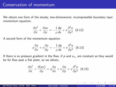
Conservation of momentum

We obtain one form of the steady, two-dimensional, incompressible boundary layermomentum equation.

∂u2

∂x +∂uv∂y = −1

ρ

dpdx + v ∂

2u∂y2 (6.12)

A second form of the momentum equation.

u ∂u∂x + v ∂u

∂y = −1ρ

dpdx + v ∂

2u∂y2 (6.13)

If there is no pressure gradient in the flow, if p and u∞ are constant as they wouldbe for flow past a flat plate, so we obtain,

∂u2

∂x +∂(uv)

∂y = u ∂u∂x + v ∂u

∂y = v ∂2u∂y2 (6.15)

John Richard Thome (LTCM - SGM - EPFL) Heat transfer - Convection 8 avril 2008 11 / 34

The skin friction coefficient

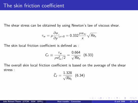
The shear stress can be obtained by using Newton’s law of viscous shear.

τw = µ∂u∂y |y=0 = 0.332µu∞x

√Rex

The skin local friction coefficient is defined as :

Cf ≡τw

ρu2∞/2

=0.664√Rex

(6.33)

The overall skin local friction coefficient is based on the average of the shearstress :

Cf =1.328√ReL

(6.34)

John Richard Thome (LTCM - SGM - EPFL) Heat transfer - Convection 8 avril 2008 12 / 34

6.3 The energy equation

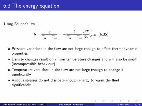
Using Fourier’s law

h =q

Tw − T∞= − k

Tw − T∞∂T∂y |y=0 (6.35)

Pressure variations in the flow are not large enough to affect thermodynamicproperties.Density changes result only from temperature changes and will also be small(incompressible behaviour).Temperature varaitions in the flow are not large enough to change ksignificantly.Viscous stresses do not dissipate enough energy to warm the fluidsignificantly.

John Richard Thome (LTCM - SGM - EPFL) Heat transfer - Convection 8 avril 2008 13 / 34

6.3 The energy equation

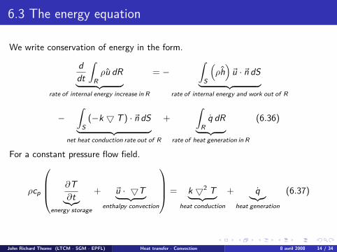
We write conservation of energy in the form.

ddt

∫Rρu dR︸ ︷︷ ︸

rate of internal energy increase in R

= −∫

S

(ρh)~u · ~n dS︸ ︷︷ ︸

rate of internal energy and work out of R

−∫

S(−k 5 T ) · ~n dS︸ ︷︷ ︸

net heat conduction rate out of R

+

∫Rq dR︸ ︷︷ ︸

rate of heat generation in R

(6.36)

For a constant pressure flow field.

ρcp

∂T∂t︸︷︷︸

energy storage

+ ~u · 5T︸ ︷︷ ︸enthalpy convection

= k 52 T︸ ︷︷ ︸heat conduction

+ q︸︷︷︸heat generation

(6.37)

John Richard Thome (LTCM - SGM - EPFL) Heat transfer - Convection 8 avril 2008 14 / 34

6.3 The energy equation

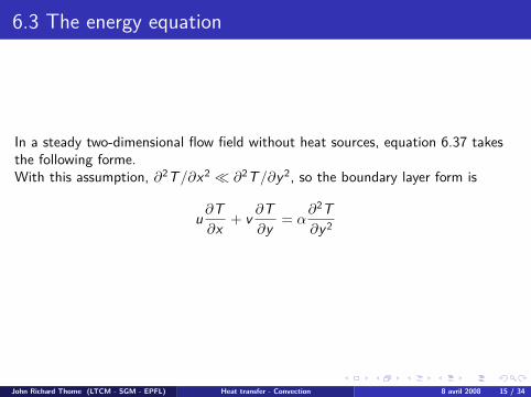
In a steady two-dimensional flow field without heat sources, equation 6.37 takesthe following forme.With this assumption, ∂2T/∂x2 � ∂2T/∂y2, so the boundary layer form is

u ∂T∂x + v ∂T

∂y = α∂2T∂y2

John Richard Thome (LTCM - SGM - EPFL) Heat transfer - Convection 8 avril 2008 15 / 34

6.4 The Prandtl number and the boundary layer thickness

To look more closely at the implications of the similarity between the velocity andthe thermal boundary layers.

h = fn(k, x , ρ, cp, µ, u∞)

We can find the following number by dimension analysis.Prandtl number

Pr ≡ ν

α

Relative effectiveness of momentum and energy transport by diffusion in thevelocity and thermal boundary layers where for laminar flow.Relationship with other dimensionless number.

Nux = fn(Rex ,Pr)

John Richard Thome (LTCM - SGM - EPFL) Heat transfer - Convection 8 avril 2008 16 / 34

6.4 The Prandtl number and the boundary layer thickness

For simple monatomic gases, Pr = 23 .

For diatomic gases in which vibration is unexcited, Pr = 57 .

As the complexity of gas molecules increase, Pr approaches an upper value ofunity.For liquids composed of fairly simple molecules, excluding metals, Pr is of theorder of magnitude of 1 of 10.For liquid metals, Pr is of the order of magnitude of 10−2 or less.

Boundary layer thickness, δ and δt , and the Prandtl numberWhen Pr > 1, δ > δt , and when Pr < 1, δ < δt . This is because high viscosityleads to a thick velocity boundary layer, and a high thermal diffusivity should givea thick thermal boundary layer.

δ

δt= fn

( ναonly

).

John Richard Thome (LTCM - SGM - EPFL) Heat transfer - Convection 8 avril 2008 17 / 34

6.5 Heat transfer coefficient for laminar, incompressibleflow over a flat surface

The following equation expresses the conservation of thermal energy in integratedform.

ddx

∫ δt

0u(T − T∞)dy =

qwρcp

(6.47)

Predicting the temperature distribution in the laminar thermal boundarylayer

T − T∞Tw − T∞

= 1− 32yδt

+12

(yδt

)3(6.50)

John Richard Thome (LTCM - SGM - EPFL) Heat transfer - Convection 8 avril 2008 18 / 34

Predicting the heat flux in the laminar boundary layer

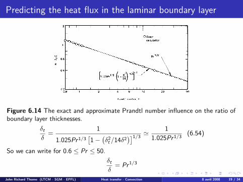
Figure 6.14 The exact and approximate Prandtl number influence on the ratio ofboundary layer thicknesses.

δtδ

=1

1.025Pr1/3[1−

(δ2

t /14δ2)]1/3 '

11.025Pr1/3 (6.54)

So we can write for 0.6 ≤ Pr ≤ 50.δtδ

= Pr1/3

John Richard Thome (LTCM - SGM - EPFL) Heat transfer - Convection 8 avril 2008 19 / 34

Predicting the heat flux in the laminar boundary layer

The following expression gives very accurate results under the assumptions onwhich it is based : a laminar two-dimensional boundary layer on a flat surface,with Tw constant and 0.6 ≤ Pr ≤ 50

Nux = 0.332Re1/2Pr1/3 (6.58)

High Pr At high Pr, equation 6.58 is still close correct. The exact solution is

Nux → 0.339Re1/2x Pr1/3, Pr →∞

John Richard Thome (LTCM - SGM - EPFL) Heat transfer - Convection 8 avril 2008 20 / 34

Some other laminar boundary layer heat transfer equations

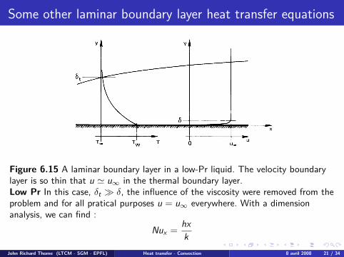
Figure 6.15 A laminar boundary layer in a low-Pr liquid. The velocity boundarylayer is so thin that u ' u∞ in the thermal boundary layer.Low Pr In this case, δt � δ, the influence of the viscosity were removed from theproblem and for all pratical purposes u = u∞ everywhere. With a dimensionanalysis, we can find :

Nux =hxk

John Richard Thome (LTCM - SGM - EPFL) Heat transfer - Convection 8 avril 2008 21 / 34

Some other laminar boundary layer heat transfer equations

We can define a new dimensionless number.Peclet number

Pex ≡ RexPr =u∞xα

(6.61)

Peclet number can be interpreted as the ratio of heat capacity rate of fluid inthe b.l. to axial heat conductance of b.l.The exact solution of the boundary layer equations gives, in this case : ForPex ≥ 100, Pr ≤ 1

100 , Rex ≥ 104.

Nux = 0.565Pe1/2x (6.62)

NuL = 1.13Pe1/2L

John Richard Thome (LTCM - SGM - EPFL) Heat transfer - Convection 8 avril 2008 22 / 34

Some other laminar boundary layer heat transfer equations

Churchill-Ozoe correlation : For laminar flow over a flat isothermal plate for allPrandtl numbers is the following for Pex > 100

Nux =0.3387Re1/2

x Pr1/3(1 + (0.0468/Pr)2/3

)1/4 (6.63)

And Nux = 2Nux

John Richard Thome (LTCM - SGM - EPFL) Heat transfer - Convection 8 avril 2008 23 / 34

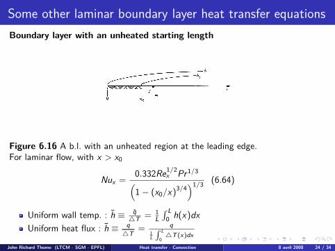
Some other laminar boundary layer heat transfer equationsBoundary layer with an unheated starting length

Figure 6.16 A b.l. with an unheated region at the leading edge.For laminar flow, with x > x0

Nux =0.332Re1/2

x Pr1/3(1− (x0/x)3/4

)1/3 (6.64)

Uniform wall temp. : h ≡ q4T = 1

L∫ L

0 h(x)dxUniform heat flux : h ≡ q

4T= q

1L

∫ L

04T (x)dx

John Richard Thome (LTCM - SGM - EPFL) Heat transfer - Convection 8 avril 2008 24 / 34

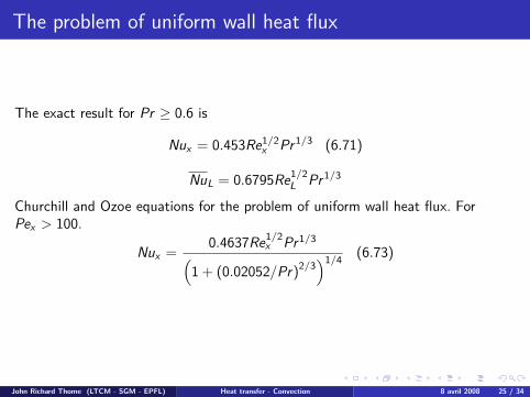
The problem of uniform wall heat flux

The exact result for Pr ≥ 0.6 is

Nux = 0.453Re1/2x Pr1/3 (6.71)

NuL = 0.6795Re1/2L Pr1/3

Churchill and Ozoe equations for the problem of uniform wall heat flux. ForPex > 100.

Nux =0.4637Re1/2

x Pr1/3(1 + (0.02052/Pr)2/3

)1/4 (6.73)

John Richard Thome (LTCM - SGM - EPFL) Heat transfer - Convection 8 avril 2008 25 / 34

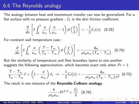
6.6 The Reynolds analogyThe analogy between heat and momentum transfer can now be generalized. For aflat surface with no pressure gradient : Cf is the skin friction coefficient.

ddx

[δ

∫ 1

0

uu∞

(uu∞− 1)d(yδ

)]= −1

2Cf (x) (6.25)

For constant wall temperature case :

ddx

[δ

∫ 1

0

uu∞

(T − T∞Tw − T∞

)d(yδt

)]=

qwρcpu∞ (Tw − T∞)

(6.74)

But the similarity of temperature and flow boundary layers to one anothersuggests the following approximation, which becomes exact only when Pr = 1.

T − T∞Tw − T∞

δ =

(1− u

u∞

)δt ⇒ −1

2Cf (x) = − qwρcpu∞ (Tw − T∞)φ2 (6.75)

The result is one instance of the Reynolds-Colburn analogy.h

ρcpu∞Pr2/3 =

Cf2 (6.76)

John Richard Thome (LTCM - SGM - EPFL) Heat transfer - Convection 8 avril 2008 26 / 34

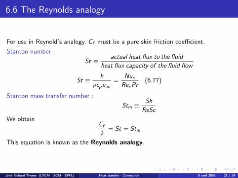
6.6 The Reynolds analogy

For use in Reynold’s analogy, Cf must be a pure skin friction coefficient.Stanton number :

St ≡ actual heat flux to the fluidheat flux capacity of the fluid flow

St ≡ hρcpu∞

=NuxRexPr

(6.77)

Stanton mass transfer number :Stm ≡

ShReSc

We obtainCf2 = St = Stm

This equation is known as the Reynolds analogy.

John Richard Thome (LTCM - SGM - EPFL) Heat transfer - Convection 8 avril 2008 27 / 34

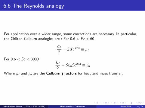
6.6 The Reynolds analogy

For application over a wider range, some corrections are necessary. In particular,the Chilton-Colburn analogies are : For 0.6 < Pr < 60

Cf2 = StPr2/3 ≡ jH

For 0.6 < Sc < 3000Cf2 = StmSc2/3 ≡ jm

Where jH and jm are the Colburn j factors for heat and mass transfer.

John Richard Thome (LTCM - SGM - EPFL) Heat transfer - Convection 8 avril 2008 28 / 34

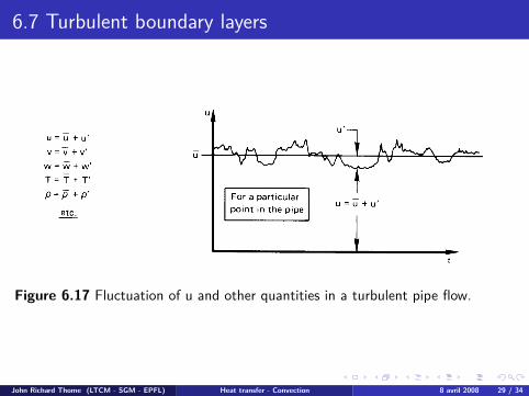
6.7 Turbulent boundary layers

Figure 6.17 Fluctuation of u and other quantities in a turbulent pipe flow.

John Richard Thome (LTCM - SGM - EPFL) Heat transfer - Convection 8 avril 2008 29 / 34

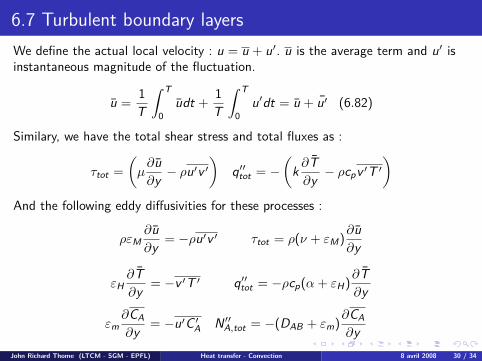
6.7 Turbulent boundary layersWe define the actual local velocity : u = u + u′. u is the average term and u′ isinstantaneous magnitude of the fluctuation.

u =1T

∫ T

0udt +

1T

∫ T

0u′dt = u + u′ (6.82)

Similary, we have the total shear stress and total fluxes as :

τtot =

(µ∂u∂y − ρu

′v ′)

q′′tot = −(k ∂T∂y − ρcpv ′T ′

)And the following eddy diffusivities for these processes :

ρεM∂u∂y = −ρu′v ′ τtot = ρ(ν + εM)

∂u∂y

εH∂T∂y = −v ′T ′ q′′tot = −ρcp(α + εH)

∂T∂y

εm∂CA∂y = −u′C ′A N ′′A,tot = −(DAB + εm)

∂CA∂y

John Richard Thome (LTCM - SGM - EPFL) Heat transfer - Convection 8 avril 2008 30 / 34

Turbulence near the wall

We define the actual local velocity : u = u + u′. u is the average term and u′ isinstantaneous magnitude of the fluctuation. For steady, incompressible, constantproperty flow with time-averaged variables, the x-momentum, energy and speciesconservation equations are :

ρ

(u ∂u∂x + v ∂u

∂y

)= −dp

dx +∂

∂y

(µ∂u∂y − ρu

′v ′)

ρcp

(u ∂T∂x + v ∂T

∂y

)=

∂

∂y

(k ∂T∂y − ρcpv ′T ′

)(u ∂CA∂x + v ∂CA

∂y

)=

∂

∂y

(DAB

∂CA∂y − v ′C ′A

)

John Richard Thome (LTCM - SGM - EPFL) Heat transfer - Convection 8 avril 2008 31 / 34

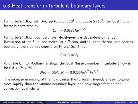
6.8 Heat transfer in turbulent boundary layers

For turbulent flow with Rex up to about 107 and above 5 · 105, the local frictionfactor is correlated by :

Cf ,x = 0.0592Re−1/5x

For turbulent flow, boundary layer development is dependent on randomfluctuation of the fluid, not molecular diffusion, and thus the thermal and speciesboundary layers do not depend on Pr and Sc. Thus :

δ ≈ δt ≈ δc

With the Chilton-Colburn analogy, the local Nusselt number in turbulent flow is :for 0.6 < Pr < 60

Nux = StRexPr = 0.0296Re4/5x Pr1/3

The increase in mixing of the fluid causes the turbulent boundary layer to growmore rapidly than the laminar boundary layer, and have larger friction andconvection coefficients.

John Richard Thome (LTCM - SGM - EPFL) Heat transfer - Convection 8 avril 2008 32 / 34

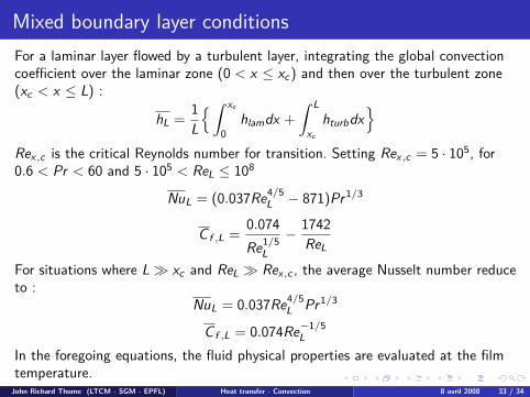
Mixed boundary layer conditionsFor a laminar layer flowed by a turbulent layer, integrating the global convectioncoefficient over the laminar zone (0 < x ≤ xc) and then over the turbulent zone(xc < x ≤ L) :

hL =1L

{∫ xc

0hlamdx +

∫ L

xc

hturbdx}

Rex ,c is the critical Reynolds number for transition. Setting Rex ,c = 5 · 105, for0.6 < Pr < 60 and 5 · 105 < ReL ≤ 108

NuL = (0.037Re4/5L − 871)Pr1/3

C f ,L =0.074Re1/5

L

− 1742ReL

For situations where L� xc and ReL � Rex ,c , the average Nusselt number reduceto :

NuL = 0.037Re4/5L Pr1/3

C f ,L = 0.074Re−1/5L

In the foregoing equations, the fluid physical properties are evaluated at the filmtemperature.John Richard Thome (LTCM - SGM - EPFL) Heat transfer - Convection 8 avril 2008 33 / 34

Guidelines of application of convection methods

Identify the flow geometry (flat plate, cylinder, etc.) ;Decide whether the local or surface average heat transfer coefficient isrequired for the problem at hand ;Choose correct reference temperature and evaluated fluid properties at thattemperature ;Calculate the Reynolds number to determine if the flow is laminar orturbulent ;Calculate the Prandle number ;Select the appropriate correlation that respects the restrictions on its use ;Double-check your design with a second correlation if application is critical tooperation when possible.

John Richard Thome (LTCM - SGM - EPFL) Heat transfer - Convection 8 avril 2008 34 / 34