(5) Multi-parameter models - Summarizingthe posterior

ST440/550: Applied Bayesian Analysis

ST440/550: Applied Bayesian Analysis (5) Multi-parameter models - Summarizing the posterior

Models with more than one parameter

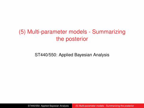
I Thus far we have studied single-parameter models, butmost analyses have several parameters

I For example, consider the normal model: Yi ∼ N(µ, σ2)with priors µ ∼ N(µ0, σ

20) and σ2 ∼ InvGamma(a,b)

I We want to study the joint posterior distribution p(µ, σ2|Y)

I As another example, consider the simple linear regressionmodel

Yi ∼ N(β0 + X1iβ1, σ2)

I We want to study the joint posterior f (β0, β1, σ2|Y)

ST440/550: Applied Bayesian Analysis (5) Multi-parameter models - Summarizing the posterior

Models with more than one parameter

I How to compute high-dimensional (many parameters)posterior distributions?

I How to visualize the posterior?

I How to summarize them concisely?

ST440/550: Applied Bayesian Analysis (5) Multi-parameter models - Summarizing the posterior

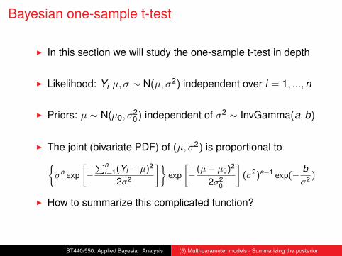
Bayesian one-sample t-test

I In this section we will study the one-sample t-test in depth

I Likelihood: Yi |µ, σ ∼ N(µ, σ2) independent over i = 1, ...,n

I Priors: µ ∼ N(µ0, σ20) independent of σ2 ∼ InvGamma(a,b)

I The joint (bivariate PDF) of (µ, σ2) is proportional to{σn exp

[−∑n

i=1(Yi − µ)2

2σ2

]}exp

[− (µ− µ0)2

2σ20

](σ2)a−1 exp(− b

σ2 )

I How to summarize this complicated function?

ST440/550: Applied Bayesian Analysis (5) Multi-parameter models - Summarizing the posterior

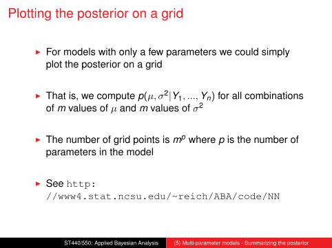
Plotting the posterior on a grid

I For models with only a few parameters we could simplyplot the posterior on a grid

I That is, we compute p(µ, σ2|Y1, ...,Yn) for all combinationsof m values of µ and m values of σ2

I The number of grid points is mp where p is the number ofparameters in the model

I See http://www4.stat.ncsu.edu/~reich/ABA/code/NN

ST440/550: Applied Bayesian Analysis (5) Multi-parameter models - Summarizing the posterior

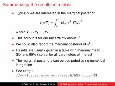
Summarizing the results in a table

I Typically we are interested in the marginal posterior

f (µ|Y) =

∫ ∞0

p(µ, σ2|Y)dσ2

where Y = (Y1, ...,Yn)

I This accounts for our uncertainty about σ2

I We could also report the marginal posterior of σ2

I Results are usually given in a table with marginal mean,SD, and 95% interval for all parameters of interest

I The marginal posteriors can be computed using numericalintegration

I See http://www4.stat.ncsu.edu/~reich/ABA/code/NN

ST440/550: Applied Bayesian Analysis (5) Multi-parameter models - Summarizing the posterior

Frequentist analysis of a normal mean

I In frequentist statistics the estimate of the mean is Y

I If σ is known the 95% interval is

Y ± z0.975σ√n

where z is the quantile of a normal distribution

I If σ is unknown the 95% interval is

Y ± t0.975,n−1s√n

where t is the quantile of a t-distribution

ST440/550: Applied Bayesian Analysis (5) Multi-parameter models - Summarizing the posterior

Bayesian analysis of a normal mean

I The Bayesian estimate of µ is its marginal posterior mean

I The interval estimate is the 95% posterior interval

I If σ is known the posterior of µ|Y is Gaussian and the 95%interval is

E(µ|Y)± z0.975SD(µ|Y)

I If σ is unknown the marginal (over σ2) posterior of µ is twith ν = n + 2a degrees of freedom.

I Therefore the 95% interval is

E(µ|Y)± t0.975,νSD(µ|Y)

I See “Marginal posterior of µ” on http://www4.stat.ncsu.edu/~reich/ABA/derivations5.pdf

ST440/550: Applied Bayesian Analysis (5) Multi-parameter models - Summarizing the posterior

Bayesian analysis of a normal mean

I The following two slides give the posterior of µ for a dataset with sample mean 10 and sample variance 4

I The Gaussian analysis assumes σ2 = 4 is known

I The t analysis integrates over uncertainty in σ2

I As expected, the latter interval is a bit wider

ST440/550: Applied Bayesian Analysis (5) Multi-parameter models - Summarizing the posterior

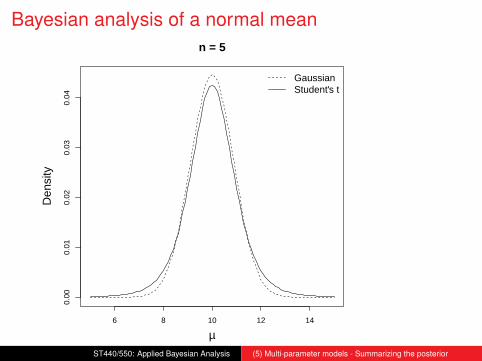
Bayesian analysis of a normal mean

6 8 10 12 14

0.00

0.01

0.02

0.03

0.04

n = 5

µ

Den

sity

GaussianStudent's t

ST440/550: Applied Bayesian Analysis (5) Multi-parameter models - Summarizing the posterior

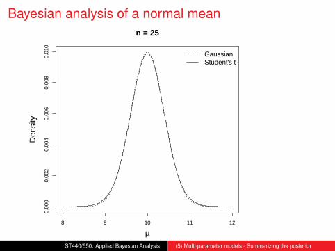
Bayesian analysis of a normal mean

8 9 10 11 12

0.00

00.

002

0.00

40.

006

0.00

80.

010

n = 25

µ

Den

sity

GaussianStudent's t

ST440/550: Applied Bayesian Analysis (5) Multi-parameter models - Summarizing the posterior

Bayesian one sample t-test

I The one-sided test of H1 : µ ≤ 0 versus H2 : µ > 0 isconducted by computing the posterior probability of eachhypothesis

I This is done with the pt function in R

I The two-sided test of H1 : µ = 0 versus H2 : µ 6= 0 isconducted by either

I Determining if 0 is in the 95% posterior intervalI Bayes factor (later)

ST440/550: Applied Bayesian Analysis (5) Multi-parameter models - Summarizing the posterior

Methods for dealing with multiple parameters

I In this case, we were able to compute the marginalposterior in closed form (a t distribution)

I We were also able to compute the posterior on a grid

I For most analyses the marginal posteriors will not be anice distributions, and a grid is impossible if there aremany parameters

I We need new tools!

ST440/550: Applied Bayesian Analysis (5) Multi-parameter models - Summarizing the posterior

Methods for dealing with multiple parameters

Some approaches to dealing with complicated joint posteriors:

I Just use a point estimate, ignore uncertainty

I Approximate the posterior as normal

I Numerical integration

I Monte Carlo sampling

ST440/550: Applied Bayesian Analysis (5) Multi-parameter models - Summarizing the posterior

MAP estimation

I Summarizing an entire joint distribution is challenging

I Sometimes you don’t need an entire posterior distributionand a single point estimate will do

I Example: prediction in machine learning

I The Maximum a Posteriori (MAP) estimate is the posteriormode

θMAP = argminθ

p(θ|Y)

I This is similar to the maximum likelihood estimation butincludes the prior

ST440/550: Applied Bayesian Analysis (5) Multi-parameter models - Summarizing the posterior

Univariate example

Say Y |θ ∼ Binomial(n, θ) and θ ∼ Beta(0.5,0.5), find θMAP

ST440/550: Applied Bayesian Analysis (5) Multi-parameter models - Summarizing the posterior

Bayesian central limit theorem

I Another simplification is to approximate the posterior asGaussian

I Berstein-Von Mises Theorem: As the sample size growsthe posterior doesn’t depend on the prior

I Frequentist result: As the sample size grows the likelihoodfunction is approximately normal

I Bayesian CLT: For large n and some other conditionsθ|Y ≈ Normal

ST440/550: Applied Bayesian Analysis (5) Multi-parameter models - Summarizing the posterior

Bayesian central limit theorem

I Bayesian CLT: For large n and some other conditions

θ ∼ Normal[θMAP , I(θMAP)−1]

I I is Fisher’s information matrix

I The (j , k) element of I is

− ∂2

∂θj∂θklog[p(θ|Y)]

evaluated at θMAP

I We have marginal and conditional means, standarddeviations and intervals for the normal distribution

ST440/550: Applied Bayesian Analysis (5) Multi-parameter models - Summarizing the posterior

Univariate exampleSay Y |θ ∼ Binomial(n, θ) and θ ∼ Beta(0.5,0.5), find theGaussian approximation for p(θ|Y)

http://www4.stat.ncsu.edu/~reich/ABA/code/Bayes_CLT

ST440/550: Applied Bayesian Analysis (5) Multi-parameter models - Summarizing the posterior

Numerical integration

I Many posterior summaries of interest are integrals over theposterior

I Ex: E(θj |Y) =∫θjp(θ)dθ

I Ex: V(θj |Y) =∫

[θj − E(θ|Y)]2p(θ)dθ

I These are p dimensional integrals that we usually can’tsolve analytically

I A grid approximation is a crude approach

I Gaussian quadrature is better

I The Iteratively Nested Laplace Approximation (INLA) is aneven more sophisticated method

ST440/550: Applied Bayesian Analysis (5) Multi-parameter models - Summarizing the posterior

Monte Carlo sampling

I MCMC is by far the most common method of Bayesiancomputing

I MCMC draws samples from the posterior to approximatethe posterior

I This requires drawing samples from non-standarddistributions

I It also requires careful analysis to be sure theapproximation is sufficiently accurate

ST440/550: Applied Bayesian Analysis (5) Multi-parameter models - Summarizing the posterior

MCMC for the Bayesian t test

I In the one-parameter section we saw that if we knew eitherµ or σ2, we can sample from the other parameter

I µ|σ2,Y ∼ Normal[

nYσ−2+µ0σ−20

nσ−2+σ−20

, 1nσ−2+σ−2

0

]

I σ2|µ,Y ∼ InvGamma[n

2 + a, 12∑n

i−1(Yi − µ)2 + b]

I But how to draw from the joint distribution?

ST440/550: Applied Bayesian Analysis (5) Multi-parameter models - Summarizing the posterior